Article

Reducing Computational Costs of Automatic Calibration of Rainfall-Runoff Models: Meta-Models or High-Performance Computers?

1
Department of Geohydraulics and Engineering Hydrology, University of Kassel, Kurt-Wolters St. 3, 34109 Kassel, Germany
2
College of Engineering, University of Georgia, Athens, GA 30602, USA
3
Leibniz Centre for Agricultural Landscape Research (ZALF), Eberswalder Straße 84, 5374 Müncheberg, Germany
*
Author to whom correspondence should be addressed.
Water 2018, 10(10), 1440; https://doi.org/10.3390/w10101440
Submission received: 12 September 2018 / Revised: 28 September 2018 / Accepted: 3 October 2018 / Published: 12 October 2018
(This article belongs to the Section Hydrology)

Abstract

:
Robust calibration of hydrologic models is critical for simulating water resource components; however, the time-consuming process of calibration sometimes impedes the accurate parameters’ estimation. The present study compares the performance of two approaches applied to overcome the computational costs of automatic calibration of the HEC-HMS (Hydrologic Engineering Center-Hydrologic Modeling System) model constructed for the Tamar basin located in northern Iran. The model is calibrated using the Particle Swarm Optimization (PSO) algorithm. In the first approach, a machine learning algorithm, i.e., Artificial Neural Network (ANN) was trained to act as a surrogate for the original HMS (ANN-PSO), while in the latter, the computational tasks were distributed among different processors. Due to inefficacy of preliminary ANN-PSO, an efficient adaptive technique was employed to boost training and accelerate the convergence of optimization. We found that both approaches were helpful in improving computational efficiency. For jointly-events calibrations schemes, meta-models outperformed parallelization due to effective exploration of calibration space, where parallel processing was not practical owing to the time required for data sharing and collecting among many clients. Model approximation using meta-models becomes highly complex, particularly in the presence of combining more events, because larger numbers of samples and much longer training times are required.

1. Introduction

Hydrologic process simulation models have brought about opportunities for watershed management policies and decision making analysis. However, taking advantages of these models is highly dependent upon parameter estimation in a mechanism called “calibration”. Automatic calibrations are usually carried out through linking a simulation model (e.g., a hydrological model) with heuristic evolutionary optimization algorithms. Having not guaranteed finding the global solutions, evolutionary algorithms have been considered as efficient tools for the purpose of solving highly nonlinear or non-convex equations, which are the cases many modelers encounter. Despite advantages, implementing these techniques necessitates solving thousands of functions which results in the calibration procedure becomes time-consuming. Thus, it is inevitable to benefit from some state-of-the-art methods for reducing computational costs.
Schemes used to alleviate the computational cost of simulation-optimization framework can be categorized into four broad research classes: (1) implementing meta-modeling approaches; (2) utilizing parallel computing computer architecture; (3) developing computationally efficient algorithms; and (4) using opportunistically evading models [1].
In the first class, meta-models attempt to develop and utilize cheaper “surrogates” of the costly simulation models to lessen the overall computational costs [2]. The idea of deploying an approximate model for optimization of computationally expensive functions was first propounded by Jones et al. [3]. This approach is per se categorized into two main groups including a sampling and control strategy. While the former focuses on how efficiently the task of experiments design functions, the latter concentrates on how to manage the surrogate model [4].
The second class, i.e., parallel processing cuts the computational cost by means of the concurrent use of more than one computer, several central processing units (CPUs), or a multi-core processor. Parallelization using multiple computers needs several computers (one as a server and the others as clients) including a local-area network which makes it possible to send and receive data. Multiple CPU-based techniques advocate a computer’s main board using several CPUs. A multi-core processor consisting of two or more independent actual central processing units acts as an integrated computing system.
The third class is designed to locate optimal or near-optimal solutions by virtue of a limited number of model evaluations, and finally the last class has been proposed to intelligently avoid unnecessary model evaluations.
Many studies have reported exploring methods for improving computational efficiency by implementing parallelization and meta-model techniques in water resources and rainfall–runoff modeling. Her et al. [5] and Rouholahnejad et al. [6] applied parallel computing approaches to decrease the computation cost of Soil and Water Assessment Tool (SWAT) model. Rao [7] ported a parallel platform to a two dimensional finite element hydrodynamic model and found that enhancing the efficiency was nearly proportional to the number of processors used. Muttil et al. [8] and Sharma et al. [9] utilized the parallel schemes of Shuffled Complex Evolutionary algorithm for model calibration. Zhang et al. [10] compared two machine learning algorithms namely Artificial Neural Network (ANN) [11] and Support Vector Machine (SVM) [12] for automatic calibration of the SWAT model. Mousavi and Shourian [4] presented an adaptive sequentially space filling approach — for optimization of a river basin decision support system—by which the process was adaptively performed via identifying regions needed more training. Shourian et al. [13] implemented the integrated ANN and Particle Swarm Optimization (PSO) [14] algorithm into a framework modeling for optimum water allocations on a basin scale.
Despite extensive studies conducted to bring down the computational cost of hydrological model calibrations, most analyses have evaluated one of the aforementioned classes. Comparison studies have only deployed different techniques which all fall within one category/class. However, nowadays with evolving new generation of super computers on one side, and proposing advanced methods to improve the competency of meta-models on the other side, the outperformance of one approach to the other remained unsolved.
To fill the above-mentioned lacuna, this study aims to compare the performance of two well-known techniques: meta-model and parallel processing to reduce the computational costs for the purpose of automatic calibration of the Hydrologic Engineering Center-Hydrologic Modeling Systems (HEC-HMS) using PSO (hereafter, HMS-PSO). Owing to limitations of calibration techniques available in HMS, it is of paramount importance to benefit from high-skill optimization algorithms to boost up the auto-calibration of this versatile hydrologic event-based model [15,16]. While auto-calibration of HMS is a fascinating subject, like for many other hydrological models [15], a dramatic rise in computational cost has stagnated applicability of such schemes, particularly when it comes to simulation of hydrographs stemmed from multi-event storms. Therefore, to accelerate the calibration process, two approaches were put into practice. In the first approach, ANN, deploying a sequential sampling strategy, was used to approximate HMS, while in the second application, parallel computing was implemented. The results of both methods were presented and their pros and cons of each one was discussed as well.

2. Material and Methods

2.1. The Hydrologic Modeling System

HMS is developed by the Hydrologic Engineering Center of the United States Army Corps of Engineers and widely used as a standard and versatile model for hydrologic simulations [17]. HEC-HMS, known for being a semi-distributed conceptual hydrological model, simulates discharge hydrographs. The required inputs include: daily precipitation and physiographic information of the watershed to simulate time series of discharge as output [18]. The model architecture consists of a watershed model, meteorological model, control specifications, and input data (time series data) [18]. Except for the soil moisture accounting model, all other hydrologic models used in HMS are event-based. Direct runoff is converted to a discharge hydrograph by a user-selected transformation model. The transform algorithms encompass various unit-hydrograph approaches, the Clark time-area method, and a kinematic wave model. The model is also able to estimate downstream processes such as channel and reservoir routing [16].

2.2. Particle Swarm Optimization

PSO is a population-based optimization technique introduced by Eberhart and Kennedy [14]. It was firstly propounded by collective and social behavior of bird flocking or fish shoaling [19]. The PSO algorithm is initialized with a population (swarm) of random solutions (particles) and searches for optima by updating particles’ locations (values) within the parameters space. The algorithm updates the particle’s locations in each iteration through two best particles including (1) “Pbest” which is the best solution achieved so far by a particle and (2) “Gbest” that is the best solution obtained so far among all particles in the swarm. After determining the Gbest and Pbest values, each particle updates whose velocity and position according to Equations (1) and (2):
  V i j ( t ) =   W e × V i j ( t 1 ) + C 1 × r a n d × [ P b e s t i j ( t ) X i j ( t 1 ) ] + C 2 × r a n d × [ G b e s t j X i j ( t 1 ) ]  
  X i j ( t ) = X i j ( t 1 ) + V i j ( t )  
where i states the particle’s number in a swarm, j is the particle’s dimension (here number of parameters) and t is the iteration number. Vij and Xij are particle’s velocity and positions respectively. The velocity drives the optimization process by reflecting experiential knowledge. We is the weighting factor and C1 and C2 are learning factors. The total numbers of particles and also maximum iterations assumed for PSO algorithm were 18 and 200, respectively. Mean Square Error (MSE) was selected as a statistic metric to assess the degree of match between the measured and simulated series of the variable of interest (here discharge).
One shortcoming of the PSO algorithm is the stagnation of particles before a good or near-global optimum is reached. To overcome this issue, algorithm was equipped with Turbulent PSO [20] and elitist-mutation strategies [21]. By using the Turbulent PSO strategy, lazy particles are triggered and allowed to better explore solutions. To do so, the velocities of lazy particles namely velocities which are smaller than a threshold Vc are updated as follows:
  V i j = { V i j i f | V i j | V c u ( 1 , 1 ) V m a x ρ i f | V i j | V c  
where μ(−1,1) is a random number, ρ states a scaling factor which controls the domain of particle’s oscillation with respect to Vmax.
Likewise, by applying the elitist-mutation strategy, the worst particles in the swarm are pre-determined their positions are replaced with that of the mutated Gbest particle [21]. This process of random perturbation will lead to an improved solution resulted from maintaining diversity in the population and exploring new regions in the whole search space. More details on implementing these two strategies are explained by Kamali et al. [16].

2.3. Parallel Processing Technique

In the current study, parallel processing was based on distributing simulations amongst three, six, and nine computers bearing the same configuration. The 18 particles of each iteration were divided by the number of PCs involved in the procedure. The PC, recognized as server, sent particle to different clients and the results (simulated discharge) were received after running the HMS model. The major advantage of the implemented parallelization was that the server could participate to the simulation process. In such a method, the available PCs are efficiently used. This leads to a reduction in total simulation time. Here, the used desktop PCs were equally configured as follow: Windows 7 Ultimate 32-bit, 3.00 GHz processor (2 CPUs), 2 GB RAM. The parallelization tasks (distributing simulations among PCs and collecting the outputs) were undertaken by executing a program written in the C# language. Figure 1 illustrates the schematic representation of parallel processing for the HMS calibration.

2.4. Artificial Neural Network (ANN)

ANN is accepted as a universal approximator for its ability in representation of both linear and complex non-linear relationships. The algorithm is applied to many fields and particularly time series prediction, classification, pattern recognition as well as model’s function approximation [22]. The input data vector (here HMS parameters) is connected to the objective function used in this study namely MSE values through a number of processing elements called Neurons [11]. There are different types of neural network architectures. Among them, the popular Multi-layer Perceptrons (MLPs) is the most well-known algorithm. A MLP network consists of an input layer, one or more hidden layers of computation nodes, and one output layer. The input signal propagates through the network in a forward direction. It has been proven that the standard feed-forward MLP with a single hidden layer can approximate any continuous function to any desired degree of accuracy [23].
MLPs were trained by means of the Levenberg-Marquardt (LM) or damped Gauss-Newton algorithm which often have been reported to have outperformance over other nonlinear optimization methods such as the classical back-projection method [24], even though it requires more computational memory resources rather than other algorithms [25]. Moreover, in this study, Tansig referring to hyperbolic tangent sigmoid, was selected as a transfer/activation function.
To set up an ANN model, the primary goal is to come up with the optimum architecture of the ANN in order to ensure a solids and plausible relationship between the input and output variables. Ascertaining the number of layers and the number of neurons in the hidden layers is accounted for a formidable challenge [11]. Since hidden layers have a considerable impact upon the output of the interested variable (e.g., discharge) as well as the performance of the ANN, both the number of hidden layers and the number of neurons for each hidden layer should be plausibly determined. Benefiting from too few neurons in the hidden layers will lead to underfitting which can be seen once existing too few neurons in the hidden layers do not allow to sufficiently capture the signals for a complex dataset. Conversely, taking advantages of too many neurons in the hidden layers will cause overfitting where the neural network includes too much information processing capacity as the parsimonious training information is not adequate to train all the neurons in the hidden layers [11]. To find out an optimum number of hidden neurons, according to a trial-and-error procedure, some rule-of-thumb methods were taken into consideration including: (1) the number of hidden neurons should fall within the sizes of the input and output layers; (2) the number of hidden neurons should be two-third size of the input layer, plus the size of the output layer, and (3) the number of hidden neurons should be less than twice the size of the input layer [22]. Regarding the number of hidden layers, similar to most ANN engineering applications where the number of hidden layers is one [22], this number was also used to construct the ANN structure in this study. In accordance with other classical data partitioning, 70% of the total data was used for training/calibration and the remaining data, i.e., 30% of the data, was set aside for validation and test purposes.

3. Study Area and Model Set-Up

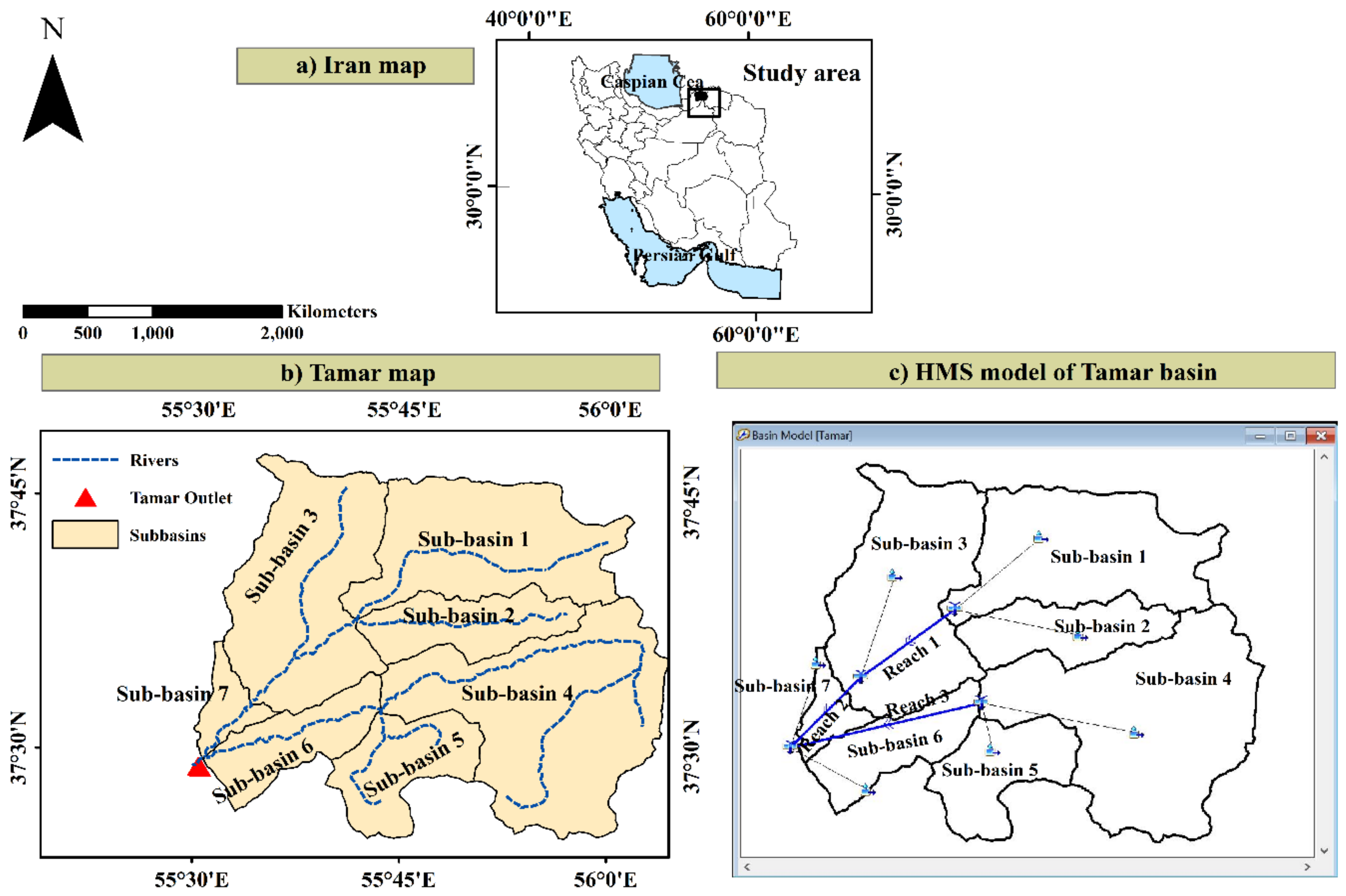
The study area is Gorganroud River Basin located in Iran extending from north-west of Khorasan province to eastern coastal of Caspian Sea (Figure 2a,b). Because of recurrent flash floods occurrence and consequent damages, there is an urgent need for a flood control management plan in this region [26]. Having a calibrated rainfall-runoff model will be an essential and inevitable asset to help policy and decision-makers better plan strategies for water resource management. The Gorganroud River Basin is divided into three sub-basins namely, Tamar, Tangrah, and Galikesh. Out of which the Tamar basin (hereafter it is called basin instead) covering an area of 1530.6 km2 was selected for this study mainly due to its reliable data (Figure 2b). To set up the HMS model of the Tamar basin, the Tamar basin was divided into seven sub-basins according to the topographic map available for this region (Figure 2c). Table 1 presents the physiographic information of these seven sub-basins.
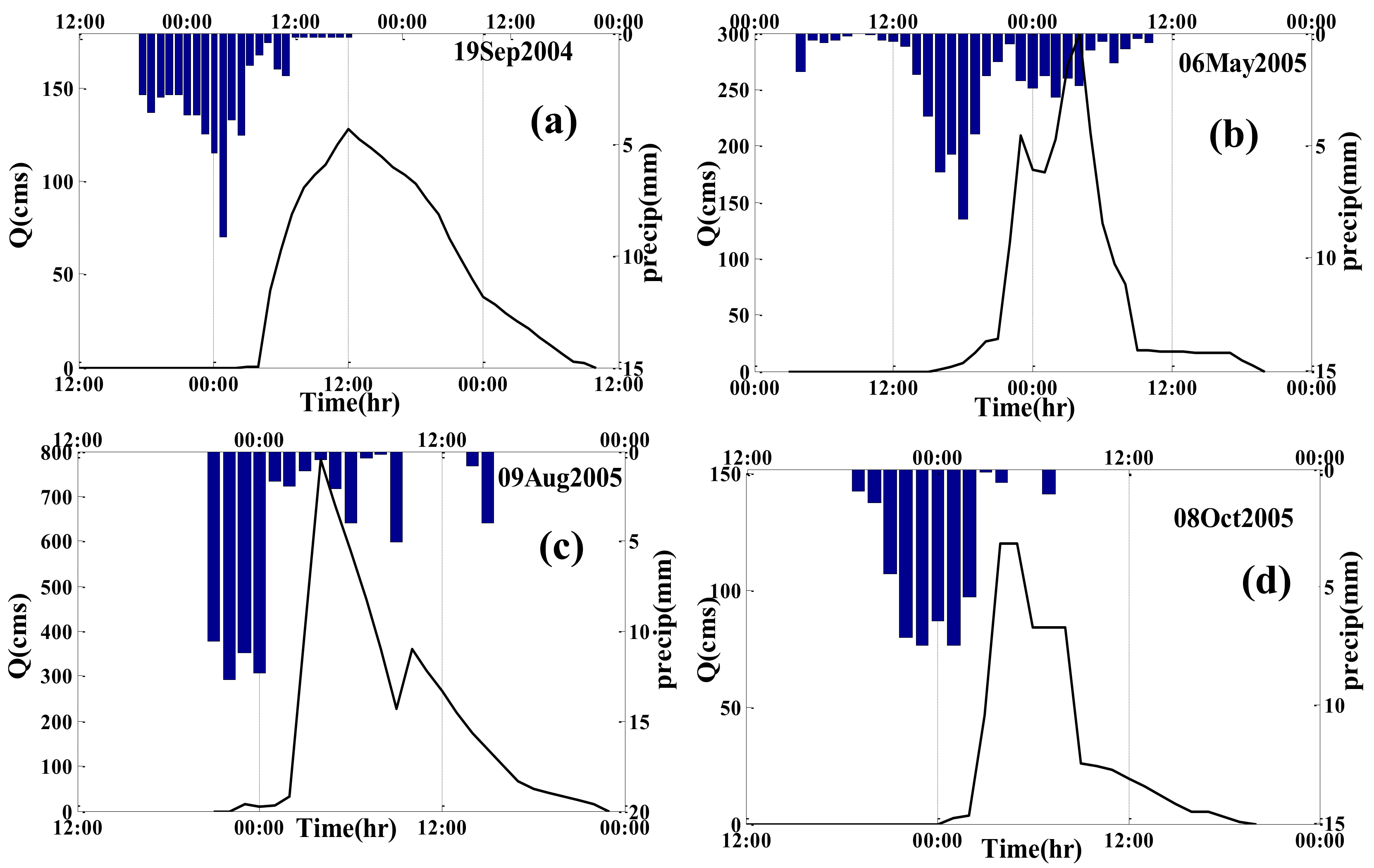
Four flood events (Event 1, Event 2, Event 3, and Event 4) were available for the region. Figure 3 gives a brief schematic of hydrographs and hyetographs which are correspondent to the four mentioned storm events. More details on the different characteristics of events are found in Kamali et al. [16].
Afterwards, among ten loss estimation algorithms available in HMS, the SCS-CN method, as the most commonly used model, was selected. The successful performance of this approach has been extensively reported by previous studies. Moreover, this method is easy to be set-up and needs readily available data [27]. The two parameters of the SCS-CN method are: Curve Number (CN) and initial abstraction (Ia) which are interrelated using the following equation:
  I a = α × ( 1000 C N 10 )  
where α is the loss coefficient. We considered CN for seven sub-basins as a calibration parameter (parameter number 1–7 in Table 2, CN1CN7). The upper and lower bounds for CN were adopted from the recommended SCS values taken from the study conducted by Kamali et al. [16]. Assuming a value of 0.2 for loss coefficient [28], the value of Ia is then calculated accordingly.
Similarly, by the fact that there are seven rainfall-runoff transformation models existing in HMS, Clark hydrograph was chosen. The method is frequently used to model the direct run-off which is generated from an individual storm. It is computed via two parameters namely time of concentration (Tc) and Clark storage coefficient (R). Tc was calculated using the SCS synthetic unit hydrograph method proposed by Chow et al. [29] and whose relationship with R is given as follows [30]:
  R R + T c = c o n s .  
By considering cons as a calibration parameter in the seven sub-basins (parameter number 8–14 in Table 2), the storage coefficient is also calibrated correspondingly. The initial values of cons deferring in each sub-basin are in range of 0.2–0.65 (Table 2). Regarding channel routing, the Muskingum model was appointed among eight routing methods available in HMS. This model was selected mainly due to containing fewer parameters which are needed to be estimated, in comparison with the other channel routing models available in HMS. Although it is a parsimonious model, it is still extensively used and incorporated in a number of river-modelling software packages [31]. The Xm of the Muskingum routing method, representing the flood peak attenuation and hydrograph shape flattering of a diffusion wave in motion, was considered as parameter numbers of three reaches (parameter number 15–17 in Table 2, Xm1–Xm3). More details on parameter calibration and the upper and lower bounds of the parameter values were further explained by Mousavi et al. [15].

4. Results

The calibration was carried out for four single storm events (Event 1, Event 2, Event 3, and Event 4) and four jointly-events including: (1) Events 1 and 2 (JEvent 1,2); (2) Events 3 and 4 (JEvent 3,4); (3) Events 1 to 3 (JEvent 1–3); and (4) all four events (JEvent 1–4). The time required for a single-event calibration on one PC is approximately 4000 s (Table 3) which increases to 18,697 s for JEvents 1–4 (containing four events). The required calibration time for single events on one PC, compared with jointly event scenarios, demonstrates that the running time is not considerable (between 3900 s and 4200 s), however this increases linearly for the jointly event scenarios calibration. This affirms the necessity of equipping the calibration process with solid techniques to noticeably bring down the simulation time.

4.1. Reducing Computational Costs Using Surrogate Model

To set up the ANN architecture as a surrogate for HMS to simulate rainfall-runoff process, 500 samples were generated by means of random and Latin Hypercube sampling (LHS) techniques. The samples were firstly normalized to improve the algorithm performance and calculation time [32]. Afterwards, the trained ANN was linked to PSO to speed up the calibration process (hereafter ANN-PSO). Comparing the results yielded by ANN-PSO with those of HMS-PSO indicates a poor performance of ANN in estimation of discharge hydrographs (Figure 4). Increasing the sample sizes by 1000, to improve the training of the constructed ANN, could not enhance the simulated hydrographs for four single events. However, as the principal objective of the current study was to cut the computational cost, adding more samples was not found to be plausible.
In order to explain the reasons for the ANN incompetence in modeling the hydrographs, we compared the ‘Gbest’ of ANN-PSO (as the surrogate model) with HMS-PSO (as the original model) at each iteration and found that in the preliminary iterations of PSO, both ANN-PSO and HMS-PSO produced the same successful results. However, after some iterations, the ‘Gbest’ particle, identified by ANN-PSO, differed from the one chosen by the original model because of the ANN failure in approximating HMS (and therefore MSE). This reveals that the ‘Gbest’ particle was located in a region that was not covered enough by the taken samples for the training of ANN. Thus, ANN did not learn adequately to simulate HMS in the vicinity of ‘Gbest’. Consequently, the MSE was not properly estimated and the particles were diverged from the space where ‘Gbest’ was located.
Increasing more samples will be probably helpful to advance the skill of the ANN-PSO model, but it can be done only at a huge computational cost which has been assumed to be prohibitive in the current study. To overcome this problem and improve the functionality of ANN without imposing high computational cost, we implemented a novel sampling strategy in which those regions of search space that require further training were identified for each iteration and ANN was re-trained adaptively (hereafter ANN-HMS-PSO). The iterative process is also called active learning. In the light of this novel method, the performance of ‘Gbest’ particle at each iteration was compared with that of the original HMS. If ‘Gbest’ was falsely identified, it was considered as a gap point in the sample sets and added to the sample repository. ANN was then re-trained using updated samples. By profiting from this technique, more detailed information near optimal solution was provided for ANN.
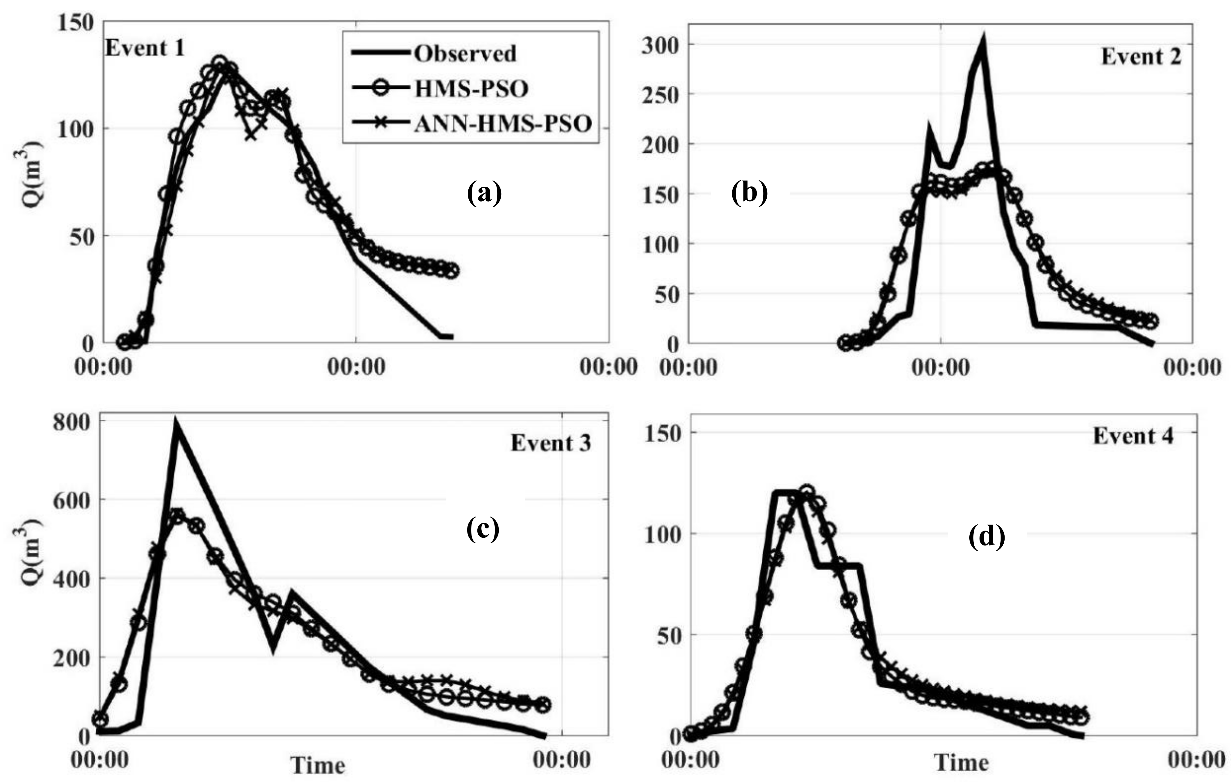
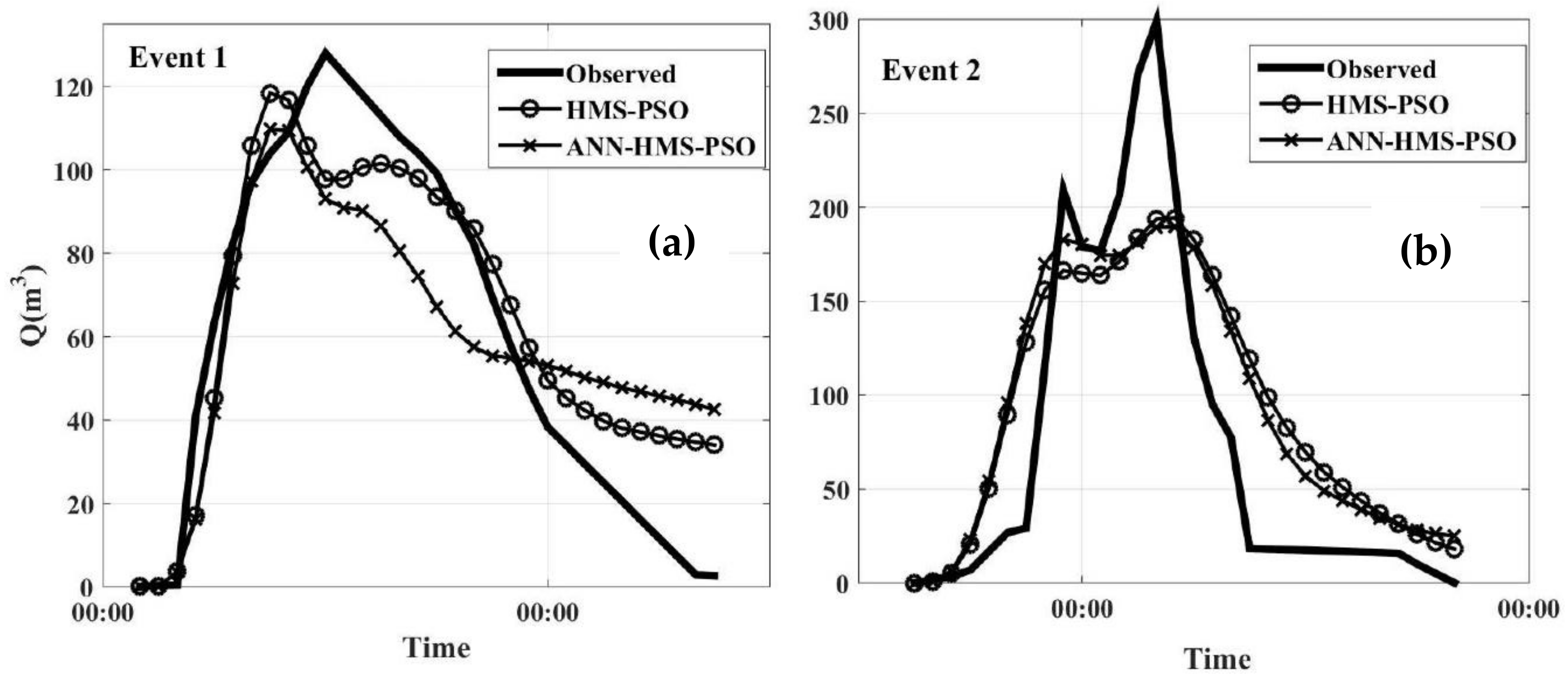
Interestingly, we also found that since the performance of ANN is adaptively enhanced for each iteration, the first ANN training can start with fewer sample size. For instance, in this study, we could decrease the initial training samples from 500 to 150, nevertheless the results still remained satisfactory. In summary, after applying adaptive sampling/active learning, the discrepancy between the simulated and observed hydrographs was mimicked (Figure 5). The results, obtained from single event calibrations, showed that the hydrographs simulated by HMS-PSO could successfully resemble those modeled by ANN-HMS-PSO for all four events. In other words, both approaches, i.e., HMS PSO and ANN-HMS-PSO approximately turned out to have the same performance.
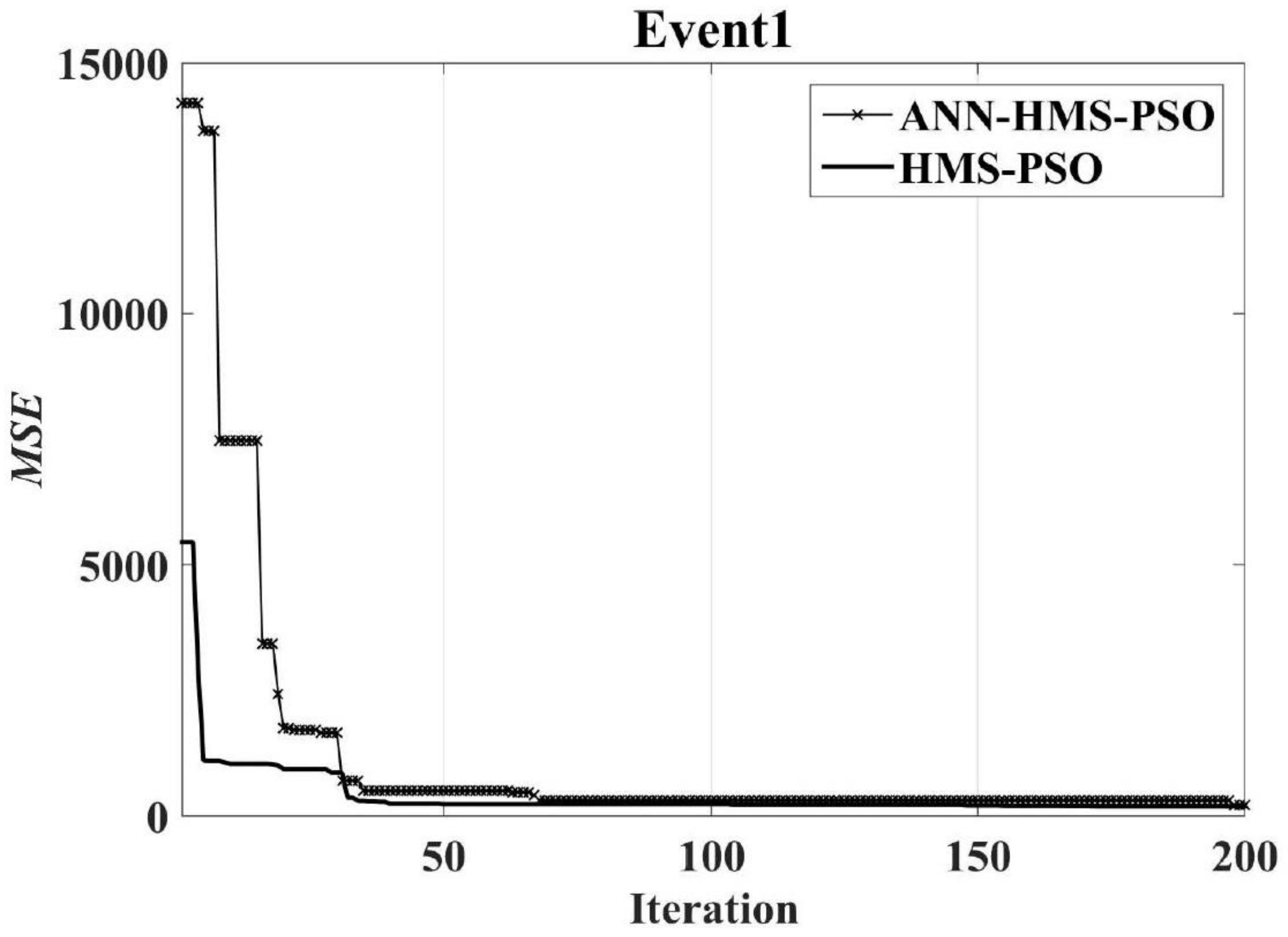
The decreasing trend in MSE over increasing the iteration, computed for both HMS-PSO and ANN-HMS-PSO models, (Figure 6) explains that in the initial iterations (e.g., 1 to 5), HMS-PSO outperformed ANN-HMS-PSO; however, after some iterations (e.g., from iteration 40 onwards for Event 1), both models have converged into nearly equal MSE values. It is important to note that in both cases the initial particles were the same.
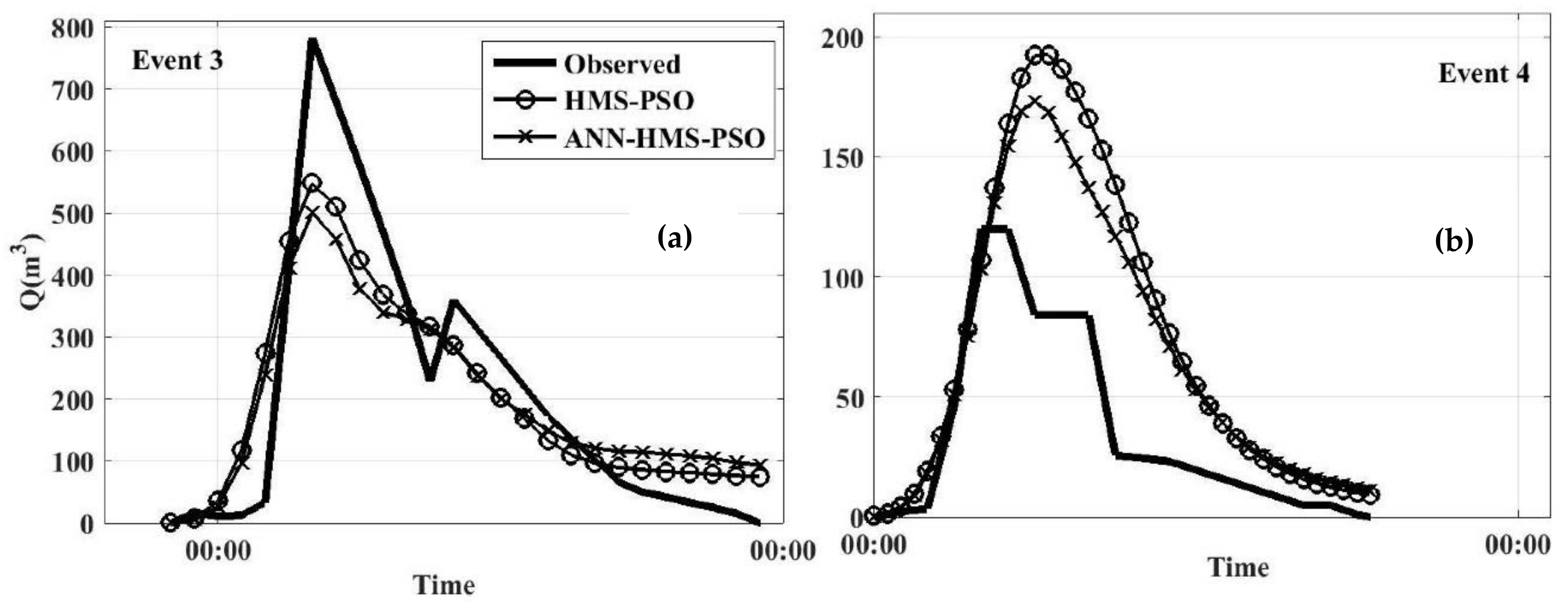
Similarly, the surrogate model, advocated by the active learning technique, promoted the hydrograph simulation for jointly event scenarios. The results, gained for JEvents 1,2, approved that despite the nearly similar MSE values (2929 for HMS-PSO versus 3062 for ANN-HMS-PSO), Event 2 was better reproduced using ANN-HMS-PSO, while HMS-PSO outperformed ANN-HMS-PSO in simulating the hydrograph of Event 1 (Figure 7 and Table 4). The same holds for JEvent 3,4 where Event 3 was better simulated by HMS-PSO, however Event 4 was more appropriately modeled by ANN-HMS-PSO, despite the fact that the same MSE was achieved (Figure 8 and Table 4).
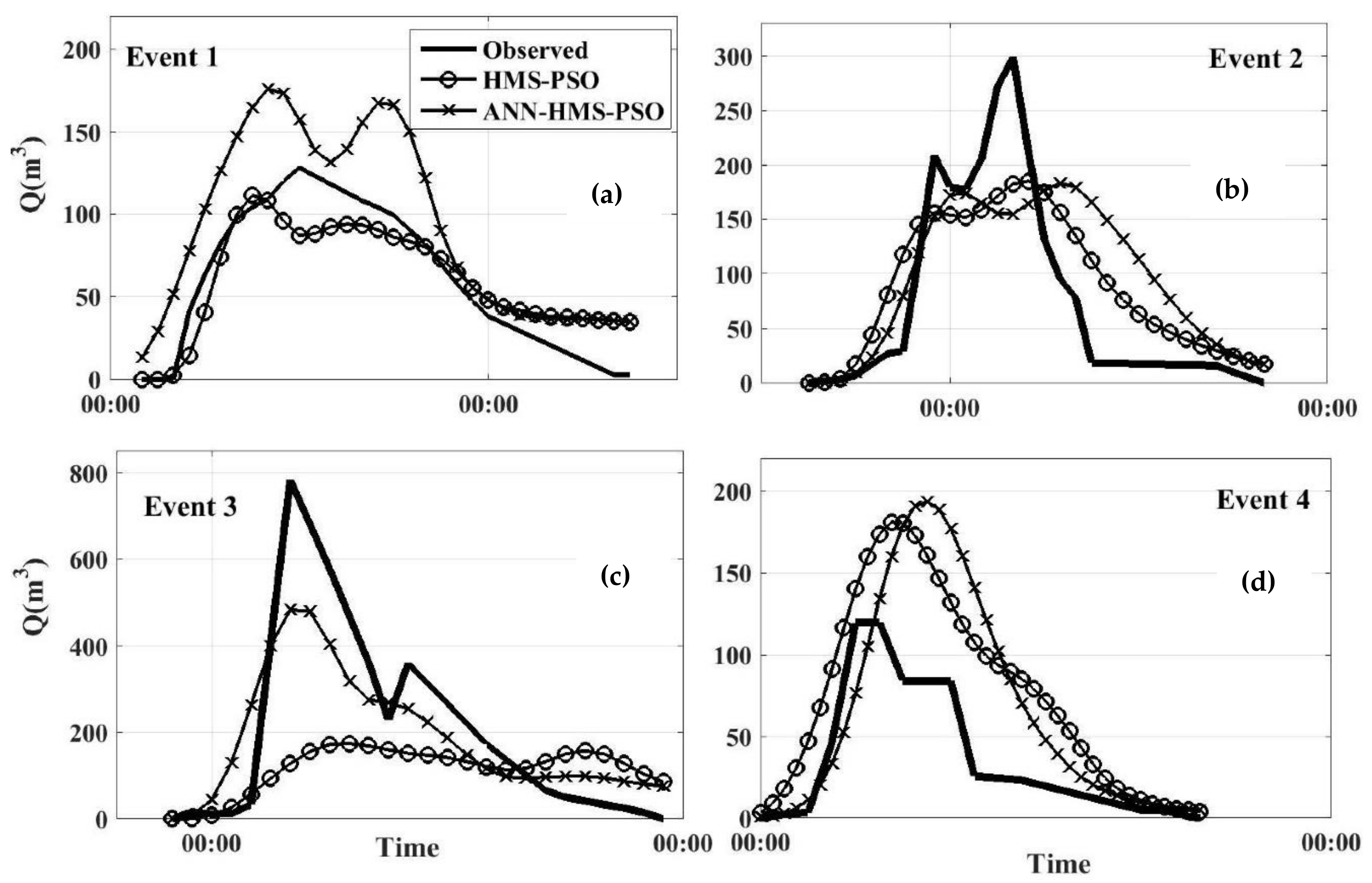
Calibration process for triple events scenario (JEvent 1–3) was also sufficiently good and the obtained results were found to be broadly similar for both HMS-PSO and ANN-HMS-PSO models (Figure 9). They yielded nearly alike MSE values (17,749 for HMS-PSO and 17,800 for ANN-HMS-PSO). The calibration of four jointly events (JEvent 1–4) presented dramatic differences between HMS-PSO and ANN-HMS-PSO (Figure 10). Interestingly, we noticed that a smaller MSE, representing a better simulation, was achieved when the ANN-HMS-PSO model was used. This revealed that the active learning technique, integrated in ANN, was beneficial to PSO in locating the search space and accordingly finding optimal solutions. This leads to avoiding PSO to be trapped in local optimal of the search space as the recurrent problem expected to occur when using optimization algorithms.

4.2. Reducing Computational Costs by Parallel Processing

The computational cost of HMS calibration was palliated by deploying a range of parallel process computing (three, six, and nine PCs). The outcomes for single event calibration determined that the required time was brought down from 4000 s to thereabouts 1500, 1000, and 750 s, when three PCs (3 PCs), six PCs (6 PCs), and nine PCs (9 PCs) were parallelized, respectively (Table 3). Under four jointly event scenarios (JEvent 1–4), this was reduced from 18,697 to about 3041 s when 6 PCs were parallelized (Table 3).
Results exhibited that the simulation time was not linearly decreased by increasing the number of PCs. In this respect, there is a noticeable difference between the simulation time of 1 PC and 3 PCs, while the same does not hold for parallel processing using 6 and 9 PCs (Figure 11). Significant attention given to reason out this non-linearity demonstrated that the resolutions of conflicting demands between the shared resources and the communication time between processors can influence the process of parallelization. As the numbers of PCs increases, the server should manage more sharing and collecting tasks. In our set-up, the server was also involved in undertaking some of the simulations, thus the time required to send and receive data from the server to clients for each iteration hampered the ideal efficiency.

4.3. Comparing the Performance of Surrogate Models and Parallel Processing

The meta-model and parallelization schemes were compared and contrasted in terms of how they can speed up the simulation time, while reducing MSE (compared with the original HMS-PSO) (Tables 5). Findings explained that both approaches were successful in reducing the calibrations time. According to the performance of the meta-models, the percentage of net simulation time (simulation time for each event) was decreased as the numbers of joint events were increased. For example, compared to the original HMS-PSO, the simulation run was speeded up by 86% for a single event calibration, but by 60% for the JEvent 1–4 scenario. Such a discrepancy (86% and 60%) can be associated with a necessity to re-training ANN for many iterations which it can be done at the cost of a higher computation cost. By employing parallelization, the speed-up rate was nearly similar for single and jointly event scenarios (e.g., between 60% and 70% when 3 PCs were parallelized) and it boosted up non-linearly when PCs were increased.
Regarding the reduction in MSE, the parallelization yielded the same results as the original HMS-PSO (as expected), whereas the meta-models simulations represented some errors (Table 5). Moreover, results indicated that an inverse relationship was found between the error in meta-models and the numbers of joint events—more events led to bigger discrepancy/error. In the other words, as the model complexity increased, owing to involving more events, the meta-model, equipped with active learning technique, helped PSO to locate particles in regions with optimal solutions.

5. Conclusions

The current study aimed to reduce the computational cost of storm-event-based rainfall-runoff simulation using parallelization and surrogate model approaches. The two approaches were taken into consideration to speed up the automatic calibration of well-known HEC-HMS hydrologic model using the PSO algorithm. Parallel processing was performed through taking advantage of simultaneous usage of PCs. The process of replacing HMS with ANN, as a surrogate model, was facilitated by virtue of active learning technique. The performance of ANN-HMS-PSO was compared with HMS-PSO in terms of the required time for simulation and the ability of the models in appropriately estimation of the hydrographs which were assessed using MSE metric.
Our Findings revealed that the hydrograph simulation, depending upon the number of the events, can last between 4000 (e.g., for Event 1) to 18,698 (e.g., for JEvents 1–4) seconds when one PC is in operation. Although the run simulation for one single event is not noticeable, by including more events to be simulated not only did the run time increase, but also the model complexity grew remarkably. Hence, reducing the computational costs, particularly for a wide range of storm events and/or time series, is inevitable and must be taken into account via some techniques.
The comparison drawn between the parallel processing scheme and the ANN meta-model explained that while both approaches could notably bring down the running time, the meta-model was found to be more efficient in complex scenarios counting more storm events (e.g., JEvents 1–4). Training ANN using an active learning technique could strongly support PSO in locating particles near optimal at a higher speed which consequently, the meta-model yielded smaller MSE. This is promising, because the sampling-based search strategies of the meta-model algorithms might require considerable time to locate optima, specifically when targeting typical hyper-dimensional parameter space of rainfall-runoff models.
Our present study compared the skill of two methods to estimate hydrographs from one to four storm events. Nevertheless, the simulation of discharge hydrographs and/or streamflow time series incorporating a large number of continuous storm events can be a research lacuna to even further assess the methods proposed in this study. Moreover, the propounded meta-model, as a surrogate for HMS, can be substituted for recently developed data-driven/machine learning techniques such as Discrete Wavelet Transform and Support Vector Machine. From the parallelization point of view, one can draw a conclusion that benefiting from a noticeable number of PCs will be offset on account of a great time allocated to send and receive data amongst the PCs. Ergo, for future studies, integration of parallelization scheme to meta-models might be a versatile tool to not only decrease a considerable fraction of the running time, but also to capture complexities expected particularly in multi-event simulations.

Author Contributions

Conceptualization, B.K.; Methodology, M.T.S.; Software, S.O.; Validation, S.O.; Investigation, M.T.S. and S.O.; Data Curation, B.K.; Writing-Original Draft Preparation, B.K. and M.T.S.; Writing-Review & Editing, M.T.S.

Funding

This research received no external funding.

Acknowledgments

The authors would like to express their gratitude towards two anonymous reviewers whose constructive comments have greatly enhanced the quality of the paper.

Conflicts of Interest

The authors declare no conflict of interest.

References

  1. Razavi, S.; Tolson, B.A.; Burn, D.H. Review of surrogate modeling in water resources. Water Resour. Res. 2012, 48, 1–32. [Google Scholar] [CrossRef]
  2. Wang, G.G.; Shan, S. Review of metamodeling techniques in support of engineering design optimization. J. Mech. Des. 2007, 129, 370–380. [Google Scholar] [CrossRef]
  3. Jones, D.R.; Schonlau, M.; Welch, W.J. Efficient global optimization of expensive black-box functions. J. Glob. Optim. 1998, 13, 455–492. [Google Scholar] [CrossRef]
  4. Mousavi, S.J.; Shourian, M. Adaptive sequentially space-filling metamodeling applied in optimal water quantity allocation at basin scale. Water Resour. Res. 2010, 46, 1–13. [Google Scholar] [CrossRef]
  5. Her, Y.; Cibin, R.; Chaubey, I. Application of Parallel Computing Methods for Improving Efficiency of Optimization in Hydrologic and Water Quality Modeling. Appl. Eng. Agric. 2015, 31, 455–468. [Google Scholar]
  6. Rouholahnejad, E.; Abbaspour, K.C.; Vejdani, M.; Srinivasan, R.; Schulin, R.; Lehmann, A. A parallelization framework for calibration of hydrological models. Environ. Model. Softw. 2012, 31, 28–36. [Google Scholar] [CrossRef]
  7. Rao, P. A parallel RMA2 model for simulating large-scale free surface flows. Environ. Model. Softw. 2005, 20, 47–53. [Google Scholar] [CrossRef]
  8. Muttil, N.; Jayawardena, A.W. Shuffled Complex Evolution model calibrating algorithm: enhancing its robustness and efficiency. Hydrol. Process. 2008, 22, 4628–4638. [Google Scholar] [CrossRef] [Green Version]
  9. Sharma, V.; Swayne, D.A.; Lam, D.; Schertzer, W. Parallel shuffled complex evolution algorithm for calibration of hydrological models. In Proceedings of the 20th International Symposium on High-Performance Computing in an Advanced Collaborative Environment (HPCS’06), St. John’s, NF, Canada, 14–17 May 2006; IEEE: Piscataway, NJ, USA, 2006. [Google Scholar]
  10. Zhang, X.S.; Srinivasan, R.; Van Liew, M. Approximating SWAT model using Artificial Neural Network and Support Vector Machine. J. Am. Water Resour. Assoc. 2009, 45, 460–474. [Google Scholar] [CrossRef]
  11. Bishop, C. Neural Networks for Pattern Recognition; Oxford University Press: New York, NY, USA, 1995; p. 482. [Google Scholar]
  12. Cortes, C.; Vapnik, V. Machine Learning; Kluwer Academic Publishers-Plenum Publisher: Dordrecht, The Netherlands, 1995; Volume 20, pp. 273–297. [Google Scholar]
  13. Shourian, M.; Mousavi, S.J.; Menhaj, M.B.; Jabbari, E. Neural-network-based simulation-optimization model for water allocation planning at basin scale. J. Hydroinform. 2008, 10, 331–343. [Google Scholar] [CrossRef] [Green Version]
  14. Eberhart, R.C.; Kennedy, J.A. New optimizer using Particle Swarm theory. In Proceedings of the Sixth International Symposium on Micro Machine and Human Science, Nagoya, Japan, 4–6 October 1995; pp. 39–43. [Google Scholar]
  15. Mousavi, S.J.; Abbaspour, K.C.; Kamali, B.; Amini, M.; Yang, H. Uncertainty-based automatic calibration of HEC-HMS model using sequential uncertainty fitting approach. J. Hydroinform. 2012, 14, 286–309. [Google Scholar] [CrossRef] [Green Version]
  16. Kamali, B.; Mousavi, S.J.; Abbaspour, K.C. Automatic calibration of HEC-HMS using single-objective and multi-objective PSO algorithms. Hydrol. Process. 2013, 27, 4028–4042. [Google Scholar] [CrossRef]
  17. U.S. Army Corps of Engineers. Hydrologic Modeling System (HEC-HMS) Applications Guide: Version 3.1.0; Hydrologic Engineers Center: Davis, CA, USA, 2008.
  18. Rauf, A.U.; Ghumman, A.R. Impact assessment of rainfall-runoff simulations on the flow duration curve of the Upper Indus River-Acomparison of data-driven and hydrologic models. Water 2018, 10. [Google Scholar] [CrossRef]
  19. Parsopoulos, K.E.; Vrahatis, M.N. Recent approaches to global optimization problems through Particle Swarm Optimization. Nat. Comput. 2002, 1, 235–306. [Google Scholar] [CrossRef]
  20. Liu, H.; Abraham, A.; Zhang, W. A fuzzy adaptive turbulent particle swarm optimization. J. Innov. Comp. Appl. 2007, 39–47. [Google Scholar] [CrossRef]
  21. Reddy, M.J.; Kumar, D.N. Optimal reservoir operation for irrigation of multiple crops using elitist-mutated particle swarm optimization. Hydrol. Sci. J. 2007, 52, 686–701. [Google Scholar] [CrossRef] [Green Version]
  22. Heaton, J. Introduction to Neural Networks for C#, 2nd ed.; WordsRU.com, Ed.; Heaton Research, Inc.: Chesterfield, MO, USA, 2008. [Google Scholar]
  23. Cybenko, G. Approximation by superpositions of a sigmoidal function. Math. Control Signal 1989, 2, 303–314. [Google Scholar] [CrossRef]
  24. Jabri, M.; Jerbi, H. Comparative Study between Levenberg Marquardt and Genetic Algorithm for Parameter Optimization of an Electrical System. IFAC Proc. Vol. 2009, 42, 77–82. [Google Scholar] [CrossRef]
  25. Adamowski, J.; Sun, K.R. Development of a coupled wavelet transform and neural network method for flow forecasting of non-perennial rivers in semi-arid watersheds. J. Hydrol. 2010, 390, 85–91. [Google Scholar] [CrossRef]
  26. UNDP. Draft Report of the Inter-Agency flood Recovery Mission to Golestan; United Nations Development Programme in Iran: Tehran, Iran, 2001. [Google Scholar]
  27. U.S. Army Corps of Engineers. Hydrologic Modeling System HEC-HMS, Technical Reference Guide; Hydrologic Engineering Center: Davis, CA, USA, 2000.
  28. USDA. Urban Hydrology for Small Watersheds; Technical Release 55; United States Department of Agriculture, Natural Resources Conservation Service, Conservation Engineering Division: Washington, DC, USA, 1986; pp. 1–164.
  29. Chow, V.T.; Maidment, D.R.; Mays, L.W. Applied Hydrology; McGraw-Hill: New York, NY, USA, 1988. [Google Scholar]
  30. Timothy, D.S.; Charles, S.M.; Kyle, E.K. Equations for Estimating Clarkunit-Hydrograph Parameters for Small Rural Watersheds in Illinois; Water-Resources Investigations Report 2000-4184; U.S. Dept. of the Interior, U.S. Geological Survey; Branch of Information Services: Urbana, IL, USA, 2000.
  31. Shaw, E.M.; Beven, K.J.; Chappell, N.A.; Lamb, R. Hydrology in Practice, 4th ed.; CRC Press: Boca Raton, FL, USA, 2010; pp. 1–546. [Google Scholar]
  32. Sola, J.; Sevilla, J. Importance of input data normalization for the application of neural networks to complex industrial problems. IEEE Trans. Nucl. Sci. 1997, 44, 1464–1468. [Google Scholar] [CrossRef]
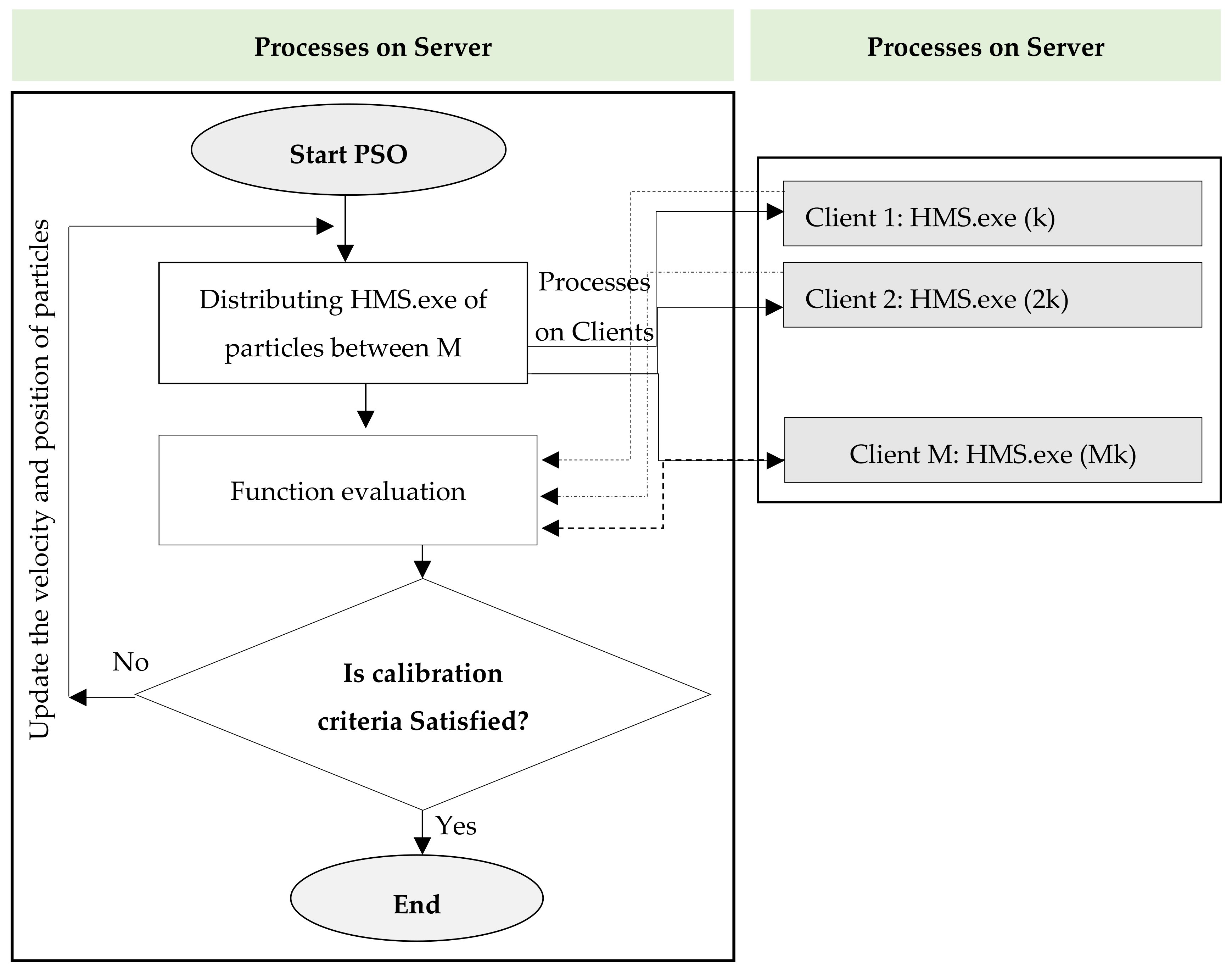
Figure 1. Schematic representation of tasks assigned to the server and different clients for automatic calibration of HEC-HMS (Hydrologic Engineering Center-Hydrologic Modeling System).
Water 10 01440 g001
Figure 2. Geographical location of the Tamar basin on Iran’s map and its representation in HEC-HMS.
Water 10 01440 g002
Figure 3. Hydrographs and hyetographs for the four flood events, occurred in a chronological order denoted by (a), (b), (c), and (d) respectively, in Tamar sub-basin. The dark blue bars exhibit rainfall and the dark curves represent the observed discharge hydrographs.
Water 10 01440 g003
Figure 4. Observed and simulated discharge hydrographs for four events, occurred on (a) 19 September 2004; (b) 6 May 2005; (c) 9 August 2005; and (d) 8 October 2005 respectively, using HMS-PSO and ANN-PSO approaches. ANN500 and ANN1000 indicate a meta-model trained with 500 and 1000 samples.
Water 10 01440 g004
Figure 5. Observed and simulated discharge hydrographs for four events scenarios occurred on (a) 19 September 2004; (b) 6 May 2005; (c) 9 August 2005; and (d) 8 October 2005 respectively.
Water 10 01440 g005
Figure 6. Convergence curve of objective function (MSE) for Event 1.
Water 10 01440 g006
Figure 7. Observed and simulated discharge hydrographs for jointly JEvent 1,2 occurred on (a) 19 September 2004; and (b) 6 May 2005 respectively.
Water 10 01440 g007
Figure 8. Observed and simulated discharge hydrographs for jointly JEvent 3,4 occurred on (a) 9 August 2005; and (b) 8 October 2005 respectively.
Water 10 01440 g008
Figure 9. Observed and simulated discharge hydrographs for jointly event scenario (JEvent 1–3) occurred on (a) 19 September 2004; (b) 6 May 2005; and (c) 9 August 2005 respectively.
Water 10 01440 g009
Figure 10. Observed and simulated discharge hydrographs for jointly event scenario (JEvent 1–4) occurred on (a) 19 September 2004; (b) 6 May 2005; (c) 9 August 2005; and (d) 8 October 2005 respectively.
Water 10 01440 g010
Figure 11. The percent of time reduction for (a) single event and (b) jointly events of parallelized HMS-PSO.
Water 10 01440 g011
Table 1. Physiographic information of seven sub-basins in the Tamar Basin.
Sub-BasinsArea (km2)Slope (%)
Sub-Basin 1307.720.99
Sub-Basin 2129.931.61
Sub-Basin 3341.113.85
Sub-Basin 4455.779.52
Sub-Basin 5135.224.8
Sub-Basin 6117.418.4
Sub-Basin 743.62.9
Table 2. The initial upper and lower bounds of the considered parameters for calibration in seven sub-basins joined by three reaches.
Parameter NumberParametersSub-BasinUpper LimitLower Limit
1–7curve number
(CN1CN7)
Sub-Basin-19160
Sub-Basin-29161
Sub-Basin-38758
Sub-Basin-48560
Sub-Basin-58450
Sub-Basin-69170
Sub-Basin-79170
8–14cons (cons1cons7) 7 Sub-Basins0.650.2
15–17(Xm1–Xm3)3 reaches0.50.2
Table 3. The required time (given in second) for calibration of different single and jointly events scenarios.
Single PCThree Parallel PCs Six Parallel PCs Nine Parallel PCs
Single eventEvent-141971579943770
Event-2391016731103732
Event-340341578969760
Event-441561836959763
Jointly eventsJEvent 1,28737264522821507
JEvent 3,48653286123091523
JEvent 1–312,815417528342259
JEvent 1–418,697542238703041
Table 4. The MSE values for jointly event scenarios using HMS-PSO and ANN-HMS-PSO models.
ScenarioEvent 1Event 2Event 3Event 4Sum
HMS-PSOJEvents 1,22692651--2920
JEvent 3,4--9075291411,989
JEvent 1–31665493911,114-17,749
JEvent 1–4360252248,572234153,797
ANN-HMS-PSOJEvents 1,25852478--3062
JEvent 3,4--10,641186312,504
JEvent 1–31573530711,571-17,800
JEvent 1–41423423612,288284021,189
Table 5. Comparison of parallelization and surrogate models performance (negative MSE means percent of error compared to original HMS-PSO and positive one means a better estimation of MSE).
Number of PCsSpeed-Up (%)Improvement in MSE Error (%)
Parallel processing Single event3PCs60The same in parallelized and unparalleled runs
6PCs76
JEvent 1,23PCs70
6PCs73
JEvent 3,43PCs67
6PCs74
JEvent 1–33PCs67
6PCs78
JEvent 1–43PCs70
6PCs80
Surrogate ModelsSingle event86.6−9.5
JEvent 1,270–75−4.8
JEvent 3,470–75−4.3
JEveny 1–360–70%−3.9
JEvent 1–460–65%+42