Understanding Morphodynamic Changes of a Tidal River Confluence through Field Measurements and Numerical Modeling


1
Division of Fluid and Experimental Mechanics, Luleå University of Technology (LTU), 97187 Luleå, Sweden
2
Division of Resources, Energy and Infrastructure, Royal Institute of Technology (KTH), 10044 Stockholm, Sweden
3
Vattenfall AB, Research and Development (R & D), Älvkarleby Laboratory, 81426 Älvkarleby, Sweden
4
College of Water Conservancy and Hydropower Engineering, Hohai University, Nanjing 210098, China
*
Author to whom correspondence should be addressed.
Water 2018, 10(10), 1424; https://doi.org/10.3390/w10101424
Submission received: 20 August 2018
/
Revised: 4 October 2018
/
Accepted: 8 October 2018
/
Published: 11 October 2018
(This article belongs to the Special Issue Applications of Computational Fluid Dynamics for Marine and Offshore Engineering)
Abstract
:A confluence is a natural component in river and channel networks. This study deals, through field and numerical studies, with alluvial behaviors of a confluence affected by both river run-off and strong tides. Field measurements were conducted along the rivers including the confluence. Field data show that the changes in flow velocity and sediment concentration are not always in phase with each other. The concentration shows a general trend of decrease from the river mouth to the confluence. For a given location, the tides affect both the sediment concentration and transport. A two-dimensional hydrodynamic model of suspended load was set up to illustrate the combined effects of run-off and tidal flows. Modeled cases included the flood and ebb tides in a wet season. Typical features examined included tidal flow fields, bed shear stress, and scour evolution in the confluence. The confluence migration pattern of scour is dependent on the interaction between the river currents and tidal flows. The flood tides are attributable to the suspended load deposition in the confluence, while the ebb tides in combination with run-offs lead to erosion. The flood tides play a dominant role in the morphodynamic changes of the confluence.
1. Background
A river confluence is a key feature of a drainage basin in terms of hydrology and geomorphology, for geological records, as well as from a habitat point of view [1]. In the confluence, two merging run-off streams often result in enhanced turbulent mixing. This has a bearing on transported sediment and its amount delivered downstream. In a long-term perspective, the flow patterns govern the morphology changes of the confluence, e.g., the scouring and sediment deposition [2].
Many studies focused on hydrodynamic patterns and morphology changes in run-off confluences. Mosley [3] was a pioneer in the research, which was further developed by Best who defined six distinct hydraulic regions in a confluence [2,4]. Those included areas of flow stagnation, flow deflection, flow separation, maximum velocity, gradual flow recovery, and shear layers. With advanced instrumentation and novel experimental design, research of river confluences evolved and focused on the separation zone and the shear layer [5,6,7,8]. Yuan et al. [9] made a review of the state of the art in hydraulic research of run-off confluences. Best [2] examined principal morphological features such as deep scour holes, bank-attached lateral bars, tributary-mouth bars, and a region of sediment accumulation in a river confluence. Other similar studies looked at the sediment and morphological aspects at non-tidal alluvial confluences [10,11,12]. They contributed to the understanding of the confluence scouring. A literature review shows that limited attention is drawn to tidal confluences with bi-directional flows [4].
In tidal environments, the confluence is also affected by tidal currents. As a result, the alluvial process in terms of erosion and deposition is different, which is an issue of concern for many practical applications, especially if the confluence is in an urban development area. Pittaluga et al. [13] investigated the morphodynamic equilibrium of alluvial estuaries, where river flows and tides meet. The complexity in a tidal confluence does not draw much attention [4,14,15]. In bi-directional flows, the shift of the dominant processes between river run-off and tides, featuring periodical changes in both magnitude and direction, induces more degrees of complexity in terms of flow patterns, sediment transport, and bed morphology change in the confluence. Ferrarin et al. [16] identified 29 scour holes at tidal channel confluences by examining their geomorphological characteristics and comparing them with scours in rivers. As a consequence of changes in the flow regime, their findings revealed, on a century scale, the morphological dynamics of scouring.
Field studies [10,11,12] and laboratory experiments [17,18,19,20] are major tools for studying sediment transport and the hydromorphic process in a confluence. In some studies, field measurements were made with tides; their purpose was to examine transport of the bed load [21,22,23]. The study of suspended load in tidal confluences is limited. One reason is attributable to the fact that it is not easy to, in a controlled manner in the laboratory, produce flow conditions of suspended load in combination with tides. Due to the complexity of the process, erosion and deposition are still not well understood [18]. Hypotheses are usually made that the origin of mid-stream scour is related to high flow velocity, strong turbulence, and the effect of shear layer or curvature-induced helical circulation [2,18,19,20].
Numerical modeling allows duplications of complex boundary conditions and prediction of different scenarios in a short time [24,25,26,27,28,29], which is also true for the study of tidal river confluences. Previous attempts were made with three-dimensional (3D) models for simulations of secondary circulations and flow variations in the vertical direction [30,31]. For a shallow confluence with a large width-to-depth ratio, a depth-averaged model is an acceptable compromise if necessary corrections of cross-circulatory motion are made [32,33,34,35].
In this research, field measurements of flow and sediment were made in the study area including the confluence. A two-dimensional (2D) morpho-dynamic model was set up, in which the cohesive suspended sediment transport was simulated. The objective was, by means of field measurements and simulations, to provide insight into the physical phenomenon that governs flow features of the tidal confluence, to describe circulatory patterns of suspended load transport, and to predict the scour-hole evolution. This study reveals the relationship between the velocity and suspended sediment movement influenced by both the run-off and the tides. The results provide reference to behaviors of tidal currents, sediment transport patterns, and fluvial process in similar situations.
The paper includes a description of the study area, field measurements of flow and sediment and data analyses, numerical formulation, model set-up with calibration and validation, major flow features, and morphological changes of the confluence.
2. Study Area
The confluence in question is called Sanjiangkou, formed by the Fenghua and the Yao River in southeast China. The stream after the confluence is called the Yong River. It is approximately 26 km upstream from the mouth into the Pacific Ocean (Figure 1). The Yao River runs into the junction roughly at a 90° angle with the other two rivers. The confluence is significantly affected by combined actions of river run-off and tidal currents. The bed load is negligibly small; the sediment transport in the rivers is mainly in form of suspended load, a common feature of many fluvial rivers [36].
Measured at the normal water surface, the width of the Fenghua River ranges from 90 to 180 m, and its average bed slope is 0.81%. The reach near the confluence is almost straight; its cross-section is nearly U-shaped. The yearly averaged run-off is 53.6 m3/s; the annual sediment discharge is 4.35 × 10⁴ tons [36].
The normal width of the Yao River ranges from 180 to 230 m. About 500 m before the confluence, a local constriction exists, with its water-surface width expanding from 140 to 180 m at the confluence. The daily run-off, as well as sediment transport, is controlled by the sluice gates located 3.3 km upstream of the confluence; the annual sediment discharge is comparatively small.
The Yong River runs roughly in the west–east direction, with its normal width ranging from 150 to 250 m. The average river-bed slope is 0.117%. Its annual mean run-off is approximately 92 m3/s (annual average run-off 2.912 × 10⁹ m3). The peak discharge of run-off and tides occurs normally during the second half of June, amounting to about 1800 m3/s. The field recording stations for river water levels (WL) and of flow and sediment (FS) are also marked in Figure 1. At the river mouth, e.g., at station WL6, the annual mean tidal range is 1.91 m; the flood and ebb durations are almost the same, approximately 6 h. The tidal asymmetry aggregates from the river mouth to the upstream. In the confluence, the ebb duration is 40 min longer than the flood duration. At station WL7, the duration difference becomes 60 min [36]. On the Yao River, the sluice gates stop the tidal propagation further upstream. As for the location of the upstream limit of current reversals along the Fenghua River, the tides affect approximately 15 km upstream of WL7/FS7; no records are available to show the run-off influence. The sediment in the river is mainly from the coastal area and is carried by the tides.
Local scouring is a typical morphological feature of the river confluence. Our concern of the bed morphology is its scour-hole evolution (Figure 1). Previous field measurements show that a scour hole, like a narrow and deep crater along the Fenghua–Yong River, exists in the confluence and its deepest point is more than 10 m below the confluence bed elevation. During the earlier years, scouring dominated the river sedimentation process. Since the 1980s, the study area was affected by a number of factors, such as the construction of the sluice gates on the Yao River and other human activities. These changes modified the hydraulic conditions and affected the erosion potential in the water system, including the confluence. Bathymetric surveys, although irregular and fragmental, show that the morphology tends to shift from erosion to deposition.
3. Field Measurements
3.1. Data Collection
To map the river and confluence topography and to record the tidal hydrological data, field surveys were carried out during two major periods, i.e., June 2015 and January 2016. The former was used for this study. The river bathymetry used in the simulations was mapped from June 2015–January 2016, which was achieved using an HY1600 bathymetric profiler (SunNav Technology Co., Ltd., Tianjin, China). The hydrological data included water level, flow velocity, flow discharge, sediment concentration, grain-size distribution, water quality, and salinity.
The water levels were monitored at seven cross-sections (WL1–WL7), five of which were along the Yong River. To measure flow velocity and suspended sediment, seven corresponding cross-sections (FS1–FS7) were arranged, each with three plumb lines (Figure 2). Their distances to the confluence (measured along the river centerline) are given in Table 1. FS5 and FS6 are a few meters apart from each other and are treated as the same section. Along each line, the sampling was made at six depths from the water surface, i.e., h = 0, 0.2H0, 0.4H0, 0.6H0, 0.8H0, and 1.0H0, where H0 (m) is the water depth at each line. All the data were recorded in one-hour intervals.
With a four-beam 600/1200-kHz RDI Workhorse acoustic Doppler current profilers (ADCPs) (Nortek group, Rud, Norway), water-flow velocities and discharges were measured. They were attached to the measurement vessels that were anchored on land. The uncertainty of the flow measurements was below ±5%. The YJD-1-type pressure sensors (Tekscan, Inc., South Boston, MA, USA) were used for the water-level measurements and their accuracy is ±1 cm. Major efforts were made to sample the suspended sediment, using point-integrative water samplers (Hoskin Scientific, Ltd., Saint-Laurent, QC, Canada). Samples of the bed load, although limited in amount, were also taken with Shipek grab samplers (Envco, Auckland, New Zealand) and their amount was calculated.
The grain-size distribution of the suspended load was analyzed using an automatic sieving device (SFY-D) (Zhonghu Scientific Ltd., Nanjing, China) and an automated laser particle-size analyzer (Mastersizer2000) (Malvern Panalytical Ltd., Worcestershire, UK). Particle sizes falling in the range between 0.0002 and 2 mm were identified. The obtained data are well suited for calibration and validation of numerical models. The field data acquired during the wet season, i.e., the second half of June 2015, were analyzed to determine the sediment features in the study area including the confluence. They are also used for calibration and validation.
3.2. Features of Suspended Sediment
For each WL and FS station, the time series of the raw measurement data were analyzed. For each time period, the average value was first obtained for each plumb line with the six points. Based on the results of the three lines, the cross-sectionally averaged value was achieved using the weighted average method.
According to the grain-size distribution, the sediment is classified as sand (0.05–2 mm), silt (0.005–0.05 mm), and clay (<0.005 mm) [37]. The field measurements show that approximately 95% of the river sediment is suspended load of cohesive silt and clay, most of which is carried into the river by the tides from the coastal area, as shown later. Table 2 shows their median grain sizes (D50) from the field data. In the spring tide, the D50 values vary from 0.005–0.009 mm for the suspended load, and from 0.008–0.017 mm for the bed load. In the neap tide, the corresponding ranges are 0.006–0.009 mm and 0.009–0.020 mm, implying that the D50 values are slightly larger.
The study area experiences a semi-diurnal tide—two nearly equal high and low tides each day, belonging to the category of incomplete standing waves. The second half of June 2015 includes 30 semi-diurnal tides, with 30 flood and ebb tides. S (kg/m3) denotes the mean sediment concentration at a cross-section. To look at its spatial changes during the period, Table 3 summarizes the time-averaged S values at FS1–FS7. The following features were observed:
- (1)
- Going upstream from FS4, including the confluence, the suspended sediment experiences a trend of decrease in concentration during the semi-diurnal tides. The maximum value of S along the Yong River always occurs at FS4, with a peak value of 2.341 kg/m3 during the spring tides.
- (2)
- At the same location during the semi-diurnal tides, the sediment concentration during the spring tide is 3–8 times higher than that during the neap tide.
- (3)
- For either the spring or neap tide at the same location, the sediment concentration of the flood tides differs from that of the ebb tides; the spring tides feature higher values than the neap tides. This implies that the spring tides govern the transport of the suspended sediment from the coastal area.
- (4)
- At FS2, the flood tides carry more sediment than the neap tides, which means that the former dominates the sediment to the confluence.
To further unveil the streamwise influence of the tides on the sediment, cross-sections FS5 (FS6) and FS2 were selected on the Yong River. The former is close to the river mouth and the latter to the confluence. Figure 3 and Figure 4 compare, for the spring and neap tides, their relationship between S and V, where V (m/s) refers to the mean flow velocity at a river cross-section, positive toward the sea [38]. A negative V value implies tidal reversal of the current.
The V and S values in the spring tides are larger than in the neap tides. S varies significantly during a tidal period, with two peaks, implying that the sediment concentration is dominated by the tides along the river. The flood tidal V and S are always out of phase with one another; the peak S appears during the flood tides. Along the river, the peak of S almost synchronizes with that of V except for during the neap tide at the river mouth. This implies that the sediment concentration is subjected to modifications by the tides at the river mouth and other oceanic processes like coastal up- and downwelling, storm surges, etc.
During the spring tide, it is the strong tidal currents that dominate the river flow and that transport the sediment toward the confluence. During the neap tide, the tide is comparatively weak; its S values are much lower (Figure 3b and Figure 4b). Judging from this, one can say that the run-off plays a major role. This leads to the non-similarity of S and V between the spring and neap tides. The tidal currents are essential for stirring sediment, modifying its peak duration, as well as its transport. If there was no tide, S would be directly proportional to the river discharge and sediment would only be diverted downstream [39].
4. Numerical Modeling
Based on the Delft3D package [40], a 2D depth-averaged model was used to help understand the complex flow features and morphology changes of the confluence. Delft3D-Flow is a separate module in the package, in which sediment motion and morphology change are coupled with the flow to simulate flow patterns and morphological changes.
4.1. Mathematical Formulation
The governing equations are based on the Navier–Stokes equations, with Leibniz integration in the vertical direction, to obtain depth-averaged flow parameters. The vertical flow acceleration is neglected, leading to the hydrostatic pressure. The turbulence shear stress is solved by the k-ε turbulence model. The river-bed stability coefficient and resistance are parameters that govern the sediment scouring and deposition. The governing equations include, therefore, mass continuity, flow motion, sediment transport, and bed deformation.
The depth-averaged continuity equation is
where H is water depth, Uξ(ξ, η) and Uη(ξ, η) (m/s) are the depth-averaged velocities in the ξ and η coordinate system, and (m) are coefficients for transformation of the curvilinear to orthogonal coordinates, q (m/s) is the global source or sink term per unit area, and t (s) is time.
The momentum equations in the ξ and η directions are
where ρ0 (kg/m3) is water density (except in the baroclinic pressure terms, variations in ρ0 are neglected), and (kg/(m2s2)) are pressure gradients, f (1/s) is the Coriolis parameter (i.e., inertial frequency), and (m/s2) refer to contributions from external sources or sinks of momentum (within the computational domain = = 0), and (m/s2) are horizontal Reynolds stresses based on the eddy viscosity concept and change in both space and time, and , , and ,, , and (N/m2) are turbulence shear stresses.
As noted from the in situ data, the bed load amount is small (below 5%). For the sake of simplification, only the cohesive suspended sediment is considered in the sediment model. The 2D transport equations for suspended load are given by
where is the function of the river-bed deformation and (m2/s) is the sediment diffusion coefficient. For large-scale river simulations, the recommended value is 10 m2/s and it was used in the simulations.
The river-bed deformation is dependent upon sediment erosion and deposition and it is expressed as
where Zb (m) is the bed elevation, γ0 (N/m) is the dry weight of suspended load, Db (kg/(m2s)) is the sediment flux of deposition from suspended load, Eb (kg/(m2s)) is the sediment flux of erosion resulting in suspended load, ωs (m/s) is the particle settling speed, Sb (kg/m3) is the sediment concentration at h = H, τb (N/m2) is the bed shear stress, τd and τe (N/m2) are the critical stresses of deposition and erosion, and M (kg/m2s) is the bed scouring rate.
4.2. Grid and Bathymetry
In an orthogonal curvilinear grid, the finite-difference method solves the partial differential equations in Delft3D-Flow. The variables of water stage, bed level, and flow velocity were arranged in a staggered grid. Delft3D-Rgfgrid, a module of the package, generated the computational grid. A quality grid is the prerequisite for reliable simulations. It should be smooth enough to minimize discretization errors; the cells should be as orthogonal as possible, with a non-orthogonal factor less than 0.02 [40]. Figure 5 shows the grid generated for the modeled area with the confluence. The total river length of the study area was about 32.5 km; the area was covered by a grid of 102,600 cells, with 760 streamwise cells and 135 transverse cells. Several grids of varying cell sizes were tested to ensure grid independent solutions. Grid independence was checked through steady-state flow calculations. From a relatively coarse grid, the mesh refinement was made both globally and locally. A larger cell density was given to the confluence area, with a minimum cell size of 5 m.
The module Delft3D-Quickin generated the river bathymetrical data. The bathymetry of the study area with the confluence is shown in Figure 6.
4.3. Boundary and Initial Conditions
There were three open boundaries in the model: two upstream inflows and one outflow. For the former (FS1 and FS7), the time series of the tributary flow discharges were specified; for the latter (WL6), the time series of the water level was given. The change in sediment concentration as a function of time was also specified at all the boundaries. Figure 7 displays the measured Q, Z, and S profiles at the three boundaries, where Q (m3/s) and Z (m) denote flow discharge and the water stage at a cross-section, respectively. The wetting and drying functions of cells in the domain were activated to reflect the rise and fall of the tides.
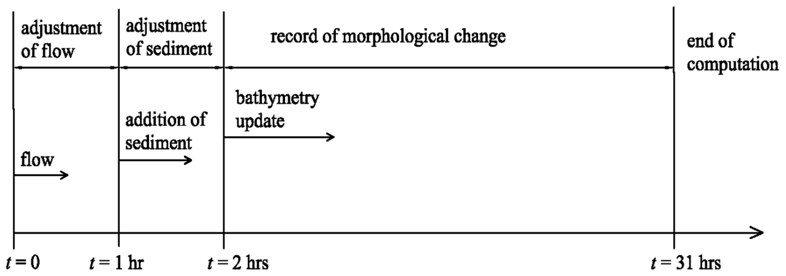
Initial conditions referred to specifications of water flow and sediment in the domain. The water level was first patched and the corresponding flow velocity was estimated by the program. Approximately one hour was taken to reach a steady-state flow. Then, the sediment concentration was patched. After another hour, the sediment conditions became steady, based on which the dynamic changes of flow and bathymetry governed by the boundary conditions were then updated. This is shown in Figure 8.
4.4. Time Step
The choice of the time step (Δt) was based on the Courant number (C), the value of which should be less than 10 [42]. It is defined as
where g (m/s2) is the acceleration due to gravity; Δt = 0.3 s was selected.
5. Model Calibration and Validation
5.1. Model Calibration
Model calibrations were based on the hourly observed data for the spring tide in 2015, occurring between 10:00 a.m. on 17 June and 4:00 p.m. on 18 June, representing 30 h in total. The model was tested with several options for boundary conditions—bed roughness, grid size, and time step. The purpose was to find a reasonable match between the observed and calculated values of flow discharge, water level, and sediment concentration. The commonly used criteria including Nash–Sutcliffe efficiency, the R-squared method, and the percent bias were also used here for the model calibration [43,44]. Table 5 shows the definitions of the error parameters and their ranges, where = measured value, = predicted value by the model, = average of measured values, = average of predicted values, and n = the total number of values.
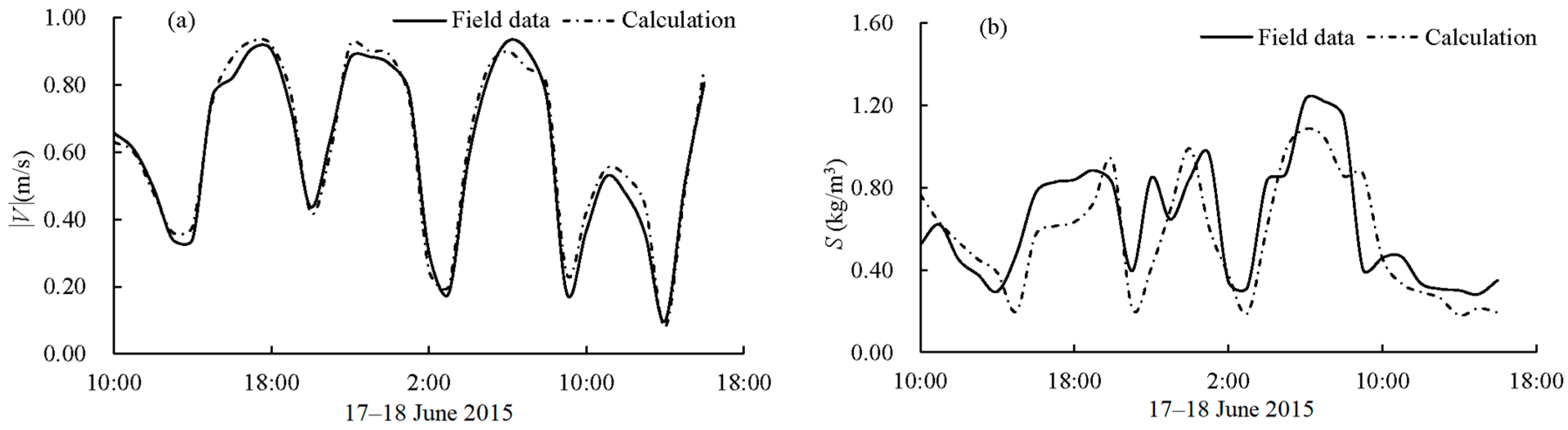
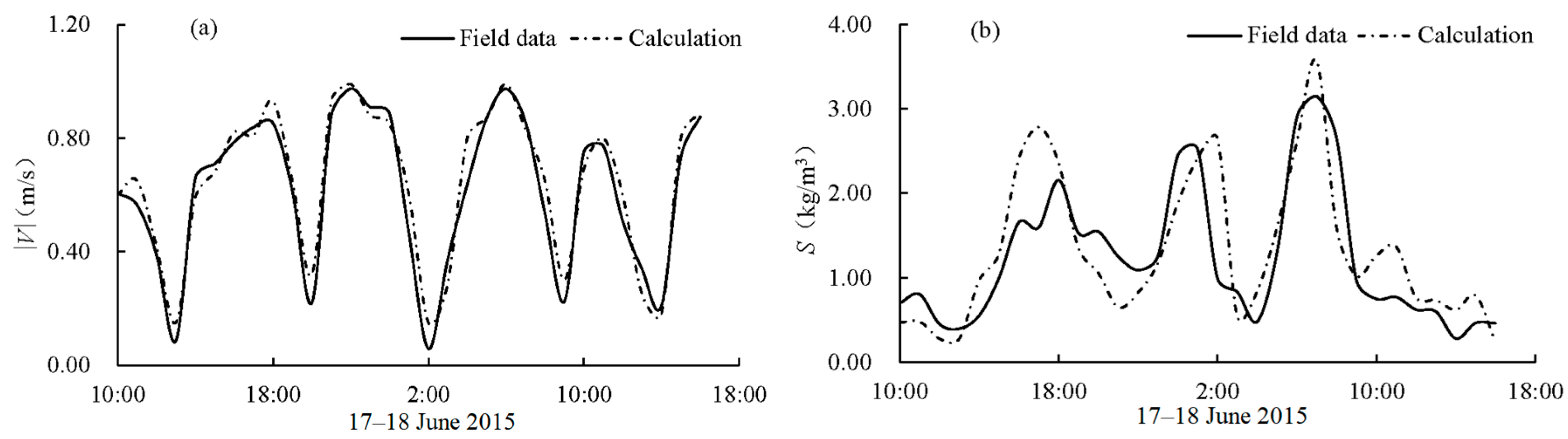
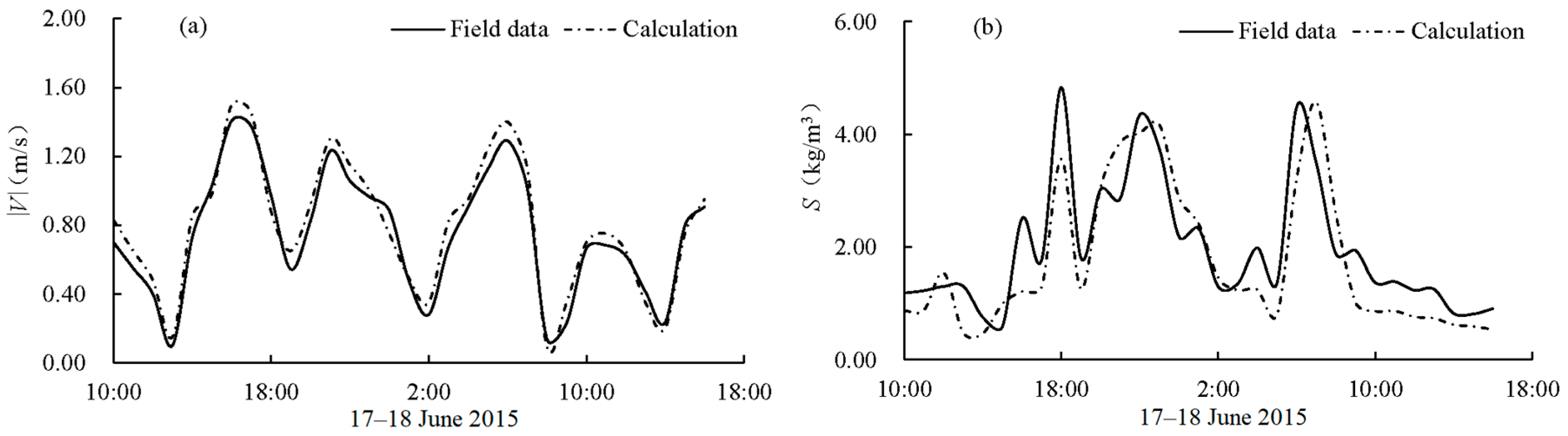
The river-bed roughness (n) is a key parameter of concern that is governed by factors, such as the river-bed morphology, flow patterns, etc. Based on trial and error, its range was finally set between 0.015 and 0.030, with 0.015–0.018 for the main channel and 0.018–0.030 for the shore beach. Figure 9, Figure 10 and Figure 11 show the final calibration results of V and S at FS2, FS3, and FS4.
For V, the computed results were in good agreement with the measured ones; the differences were negligibly small for all the stations. For S, despite certain discrepancies between them, the matches were generally satisfactory. The four S peaks within the tidal period were reasonably reproduced, in terms of both magnitude and phase. For FS2, FS3, and FS4, Table 6 shows the calibration results of the error parameters. All the values fell within the ranges required by the criteria.
5.2. Model Validation
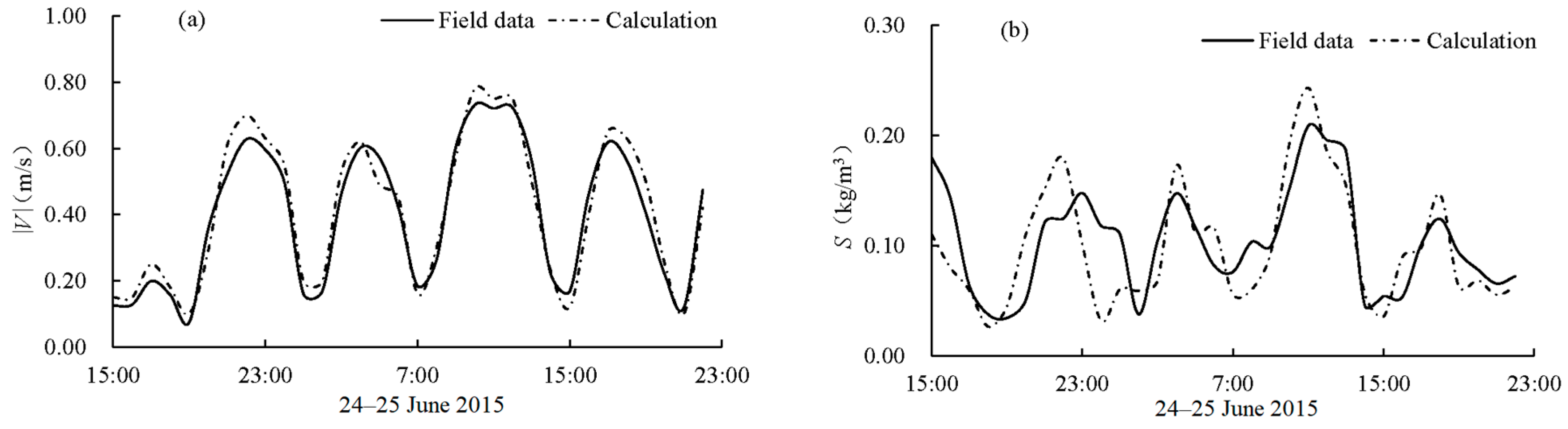
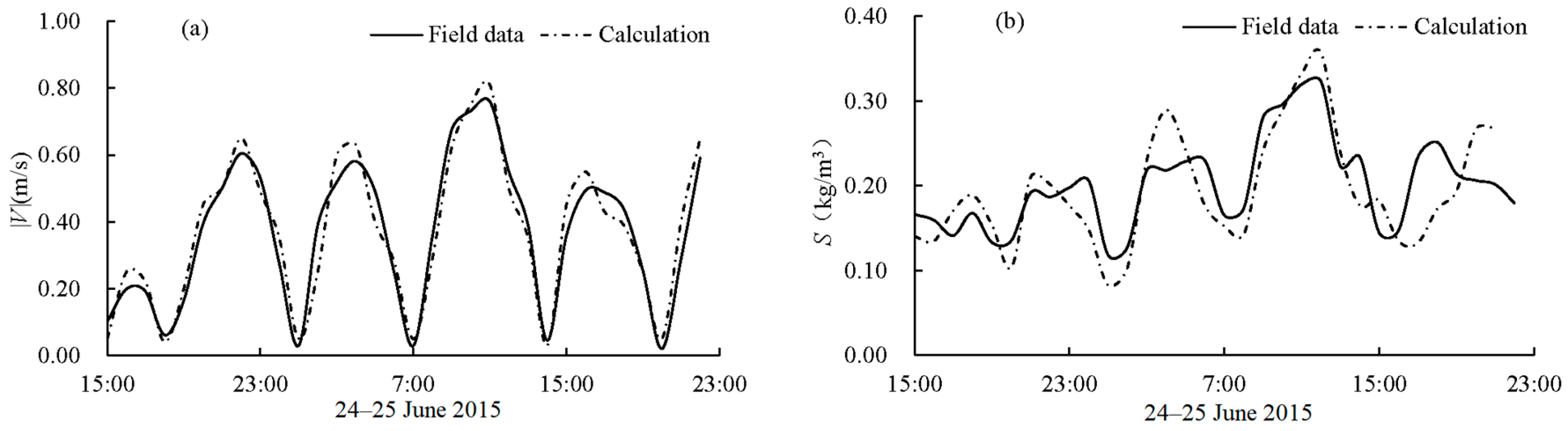
The model was validated against a neap tide that occurred during a 31-h period between 3:00 p.m. on 24 June and 10:00 p.m. on 25 June of the same year. In the validation, the procedure for result evaluations was the same as for in the calibration.
The validation results are shown in Figure 12, Figure 13 and Figure 14. The calculated V and S profiles matched well with the measured data series. Table 7 shows the validation results of the error parameters for the three stations. All the values met the requirements of the criteria. The model generated acceptable results and is suitable for prediction of flow and morphology changes of the area including the confluence.
6. Typical Flow Features
According to the statistics of the whole-year water-level data at WL6 during 2015, the tidal frequency in the wet season (the 2nd half of June) was 10%, 40%, and 25% for the spring, mid, and neap tides, respectively [45]. Under the combined action of the run-off and tides, the maximum flood and ebb tides of the spring tides dominate the sediment transport; they also characterize the flow features and they were selected to show the results.
6.1. Tidal Current Fields
When the maximum flood tide from the Yong River approached the confluence, the confluence flow saw an increase in magnitude. The flow field at the maximum flood tide is shown in Figure 15a. Current reversals occurred because the tides were stronger than the river run-off. It was a flow bifurcation. The surface flow pattern was relatively smooth in the confluence. In the Yong River, the depth-averaged flow velocities were largest (0.6–0.8 m/s). In the Fenghua and Yao rivers, the tidal currents were weak; the corresponding velocities amounted to 0.4–0.6 and 0.2–0.3 m/s, respectively. Furthermore, the tidal current flowing into the Yao River was influenced by the bend. Due to the centrifugal force [46], its mainstream was close to the concave river bank.
With the incoming maximum ebb tide from the two tributaries to the Yong River, the flow velocity reached its peak in the confluence. The tidal flow field at the maximum ebb tide is illustrated in Figure 15b. In the Yao and Yong rivers, the depth-averaged velocities were 0.7–0.9 m/s and 0.4–0.6 m/s, respectively. In the Fenghua River, the tidal current was comparatively weak with its velocity amounting to 0.3–0.5 m/s. The simulations showed that there was a small zone of flow circulation close to the left bank of the confluence. The occurrence was ascribed mainly to the confluence geometry and also to the difference in momentum between the two tributaries [47]. The relative strength of the two meeting streams plays a role in the location and size of the vortex zone. The separation zone occupies part of the channel cross-section, thus leading to a reduction in the capacity of river conveyance. It causes also sediment deposition in the zone.
The flow velocity in the confluence was smaller than the nearby velocities in the river streams. The discrepancy was attributed to the effect of the momentum offsetting. If two flows merge with each other, there is momentum exchange, which enhances the turbulent mixing, leading to energy dissipation. Moreover, the water depths in the confluence were larger, also explaining the smaller velocities.
In the confluence, comparison of the velocities at the maximum flood and ebb tides show that the latter was approximately 0.2 m/s larger than the former, which was due to the addition of the ebb tide to the run-off. The volume of the ebb tide was also larger than that of the flood tide, while, for the flood tide, the run-off and the tide were in opposite directions, thus offsetting each other. The prevalence held that the velocity of the ebb tide was higher than that of the flood tide.
In summary, parting from the water levels, the confluence flow at the maximum flood tide differed in both flow direction and magnitude from that at the maximum ebb tide, which depended on the tidal flow direction. At the ebb tide, a zone of flow separation also existed close to left river bank.
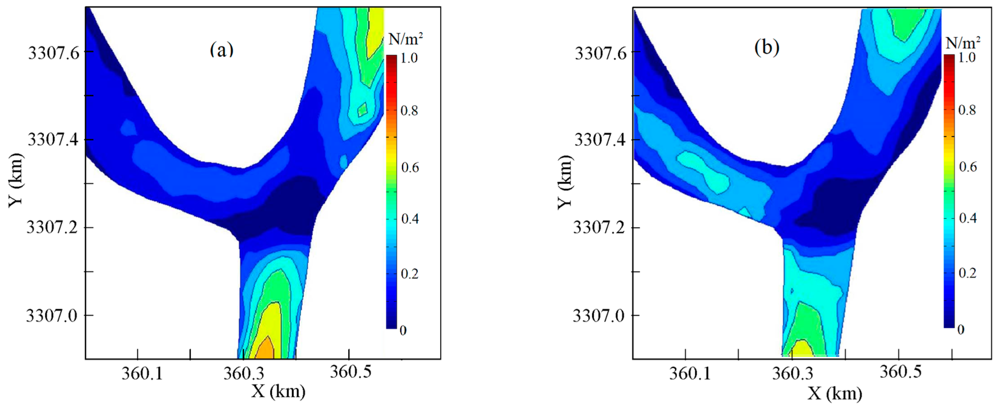
6.2. Bed Shear Stress
For a location in question, relates the flow regime to deposition and erosion patterns. It is a function of a quadratic of and the 2D Chézy coefficient C2D (m0.5/s) or an equivalent roughness length [48]. For 2D depth-averaged flows, is given by
where (m/s) is the magnitude of . C2D is expressed as
Collins et al. [48] pointed out the variability of these parameters. In a tidal confluence, the determination is complicated by factors such as confluence geometry, bed topography, and sediment. Flow perturbations make it difficult to measure in the field. Therefore, numerical models are often used for obtaining in tidal environments.
is proportional to and is also affected by H. In the confluence, the and H values were between 0.4–0.6 m/s and 6.0–17.3 m (exclusive of the scour hole). At the maximum flood and ebb tides, Figure 16 shows the distribution of the peak values. Their distributions of were similar, with some local differences. For each tide, the spatial distribution and magnitude followed the pattern of the velocity gradient distribution. For a given river, a decay was exhibited from the mainstream to the bank.
reflects the velocity gradient and is affected by both run-off and tides. The peak values occurred away from the confluence in the Fenghua and Yong rivers, which was true for both the flood and ebb tides. The occurrence of these areas was similar to the situation with only the run-off in the rivers [1,4,9].
Low values occurred in such areas as along the Yao River and in the confluence. At the confluence, the Yong and Fenghua rivers run almost along a straight line, while the Yao River intersects them at almost a right angle. As the tide comes from the Yong River, the tides are bathymetrically constrained and the bending accounts for the low values in the Yao River. links the flow conditions with sediment transport, providing indications of morphology change.
7. Morphological Changes
With the typical confluence flow features, predictions were made to look at the potential pattern of morphological changes. The construction of the sluice gates on the Yao River interrupted the natural run-off downstream. Another factor is that many wading structures were built on both rivers upstream of the confluence, which also affected the run-off in the water system. This means that the tides interact with the run-off in a different way than before; the intrusion of the tidal waves is further upstream, which probably results in more sediment deposition. Simulations were carried out to estimate the possible scenarios.
As shown earlier, the tidal currents, especially for the spring tides in wet seasons, dominate the sediment transport in the area. During the second half of June 2015, the 30-h spring tide was selected for the purpose. Along the rivers including the confluence, the start condition of the river bed corresponded to the bathymetry obtained at 10:00 a.m. on 17 June 2015. As shown in Figure 17, a long, oval-shaped scour hole exists in the confluence and extends into the Yong River. Its depth is 10.8 m at the maximum (the river bed is 6.5 m below the mean sea level, with a bed elevation of −6.5 m). In the simulation, a morphological scaling factor was used to accelerate the bed erosion and deposition, a method of common practice [39,49,50,51]. The scaling factor was set to 100, implying that the prediction period covered 125 days.
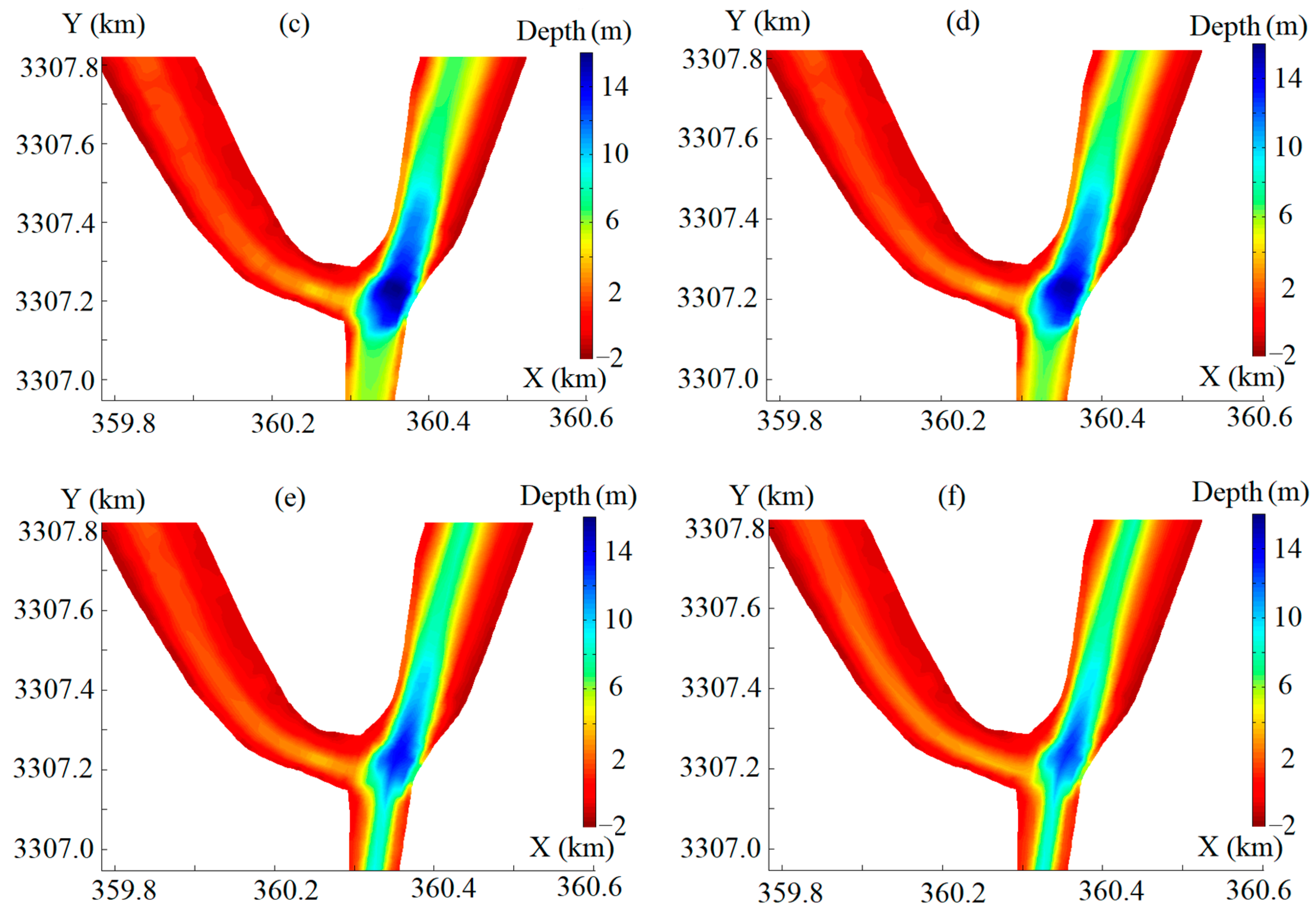
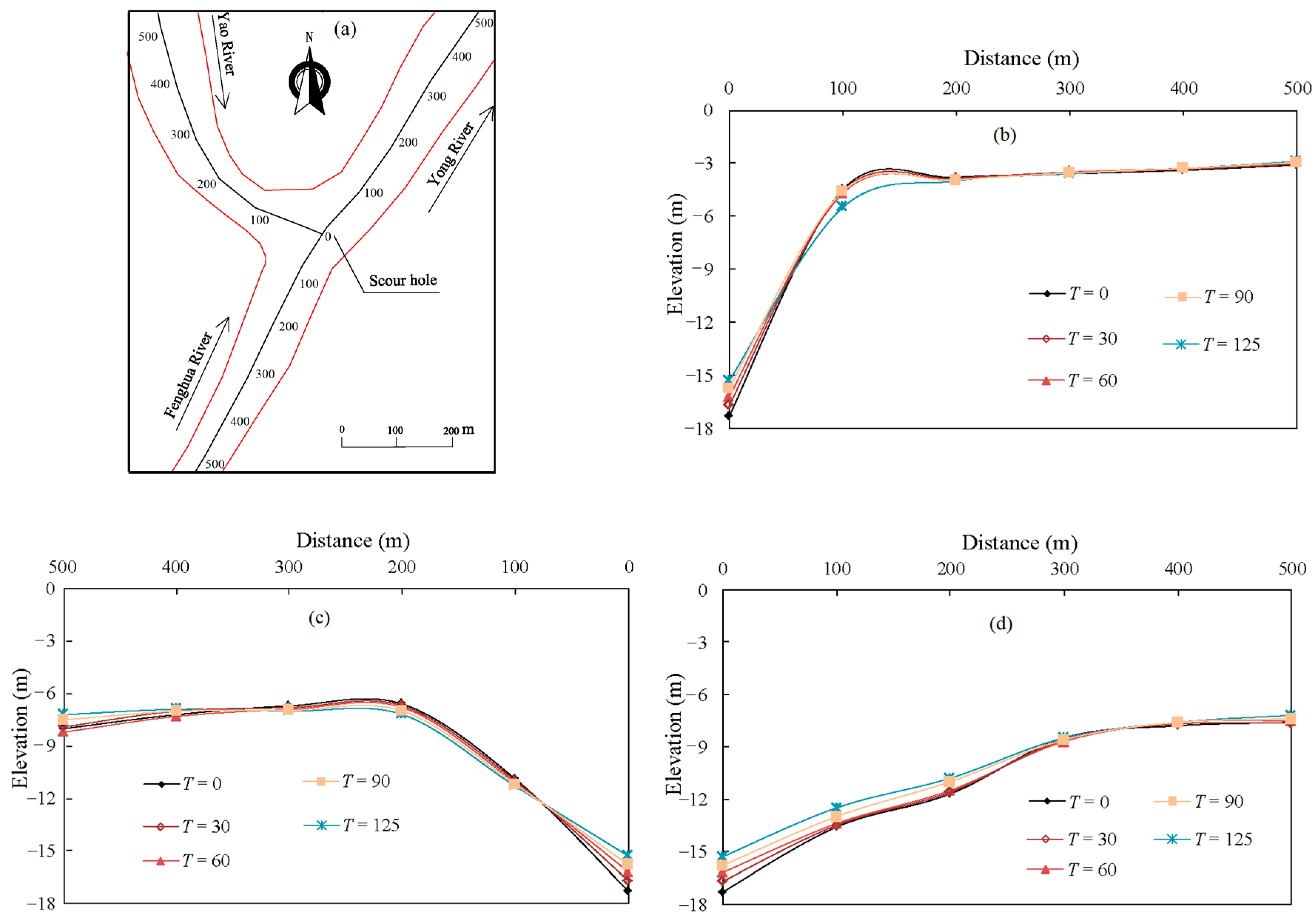
Figure 18 illustrates, in the confluence and its close vicinity, the bed evolution from T = 0, 30, 60, 90, 120, and 125 days. The results show, as time elapses, that the three river reaches were subjected to continuous siltation. The trend is in qualitative agreement with the study of the water system by Chen et al. [36], in which the cumulative influence of the wading structures, including the Yao sluice gates, bridges, and wharfs, was analyzed. Their results showed that the rivers including the confluence also suffered from gradual siltation of suspended load. Figure 19 illustrates the change in scour-hole depth and the averaged elevation of the river bed around the hole. Figure 20 shows, as a function of time, the simulated longitudinal profiles of the bed-level changes along each river at the confluence. Both the river bed and the scour hole show a tendency of gradual deposition. The hole depth was initially 10.8 m and became 9.25 m at T = 125 days.
Both the flood and ebb tides contributed to shaping the confluence scour hole. The former gave rise to deposition, while the latter led to erosion. However, the flood tide played a dominant part in the process. As a result, the scour hole shrank both upstream and downstream as time elapsed. Two factors accounted for the morphological feature. On one hand, the change was associated with the sediment availability in each river. The field measurements indicated that the flood tides carry a large amount of suspended load upstream. When flow velocity fell below 0.8 m/s, deposition occurred in the confluence area. Using morpho-sedimentological and seismo-stratigraphic data, Silva et al. explained a similar phenomenon of confluence deposition [15]. They found that the river sediment was deflected back into the river by the flood tides, thus producing the sediment deposition on the scour hole’s gentle side (downstream slope). On the other hand, the cumulative effect of river run-off and ebb tides was also attributable to the scour changes. During the ebb tides, the deposited sediment in the confluence became re-suspended and resulted in slight bed erosion. The dominance of the flood tide eventually led to the sediment deposition along the rivers inclusive of the confluence.
The Yao River also features gradual siltation, which changes its river-bed slope and lowers the sediment carrying capacity. This was also observed in the field [38]. Two plausible reasons account for it. One is ascribed to the construction of the sluice gates and the wading structures upstream. As a result, it not only intercepts the river run-off, but also deforms the tidal waves in the river. According to measurements [38], the mean high tidal level increased by 0.17 m; the mean low tidal level decreased by 0.11 m. The flood tide duration became 9 min shorter and the ebb tide duration became 9 min longer. The other reason is due to the bending toward the confluence. The flow, either during the flood or ebb tides, fails to transport the sediment downstream, thus leading to deposition along the river.
The periodic changes in the tidal flow direction induce a complex morphological regime that does not occur in unidirectional run-off flows. Concerning the sedimentation pattern, the morphologic features migrate streamwise with run-off flows [3,49]. With tidal waves, the pattern migrates both ways, which agrees with previous findings of the tides that both deposition and re-suspension take place in the confluence [52]. The analysis showcases that the flow regime is the main driver of the confluence scour evolution. The morphological changes in the confluence subjected to strong tides are closely related to the interactions between the run-off and tidal currents. However, the latter plays a dominant role and governs the sedimentation pattern.
8. Conclusions
In a river confluence subjected also to strong tidal currents, its flow and morphological changes are dependent on a number of factors, showing a complex pattern in both time and space. This study dealt with the typical features of such a confluence by means of field studies and numerical modeling.
From the sea into the Yong River, the sediment is transported by the tidal currents, especially during the spring tides. During the selected period of two years, field measurements were made to examine the sediment behaviors. The data show that approximately 95% of the sediment in the study area is suspended load. From the river mouth to its upstream including the confluence, the flow and sediment changes are not always in phase with one another; the sediment movement is significantly modified by the tides. The peak values of sediment concentration occur during both the flood and ebb tides in the rivers. Tidal currents are essential for stirring sediment, modifying its concentration and transport. If there was no tide, the sediment concentration would be directly proportional to the river flow, with the sediment diverted only downstream.
With the field measurements in the background, numerical modeling helps understand the alluvial features of the confluence. Two-dimensional simulations of suspended sediment transport were performed to simulate the sediment patterns. At the confluence, the flow at the maximum flood tides differs, in both flow direction and magnitude, from that at the maximum ebb tides. During the ebb tides, a small zone of flow circulations exists close to the left bank of the confluence. The bed shear stress is proportional to the water depth and flow velocity, and it is affected by the river-bed topography. Its distribution reflects the sediment erosion potential in the confluence.
By means of a morphological scale factor, the scour formation in the confluence was predicted. The initial hole in the confluence, extending along the Fenghua and Yong rivers, becomes gradually deposited as time elapses. The shifting tidal directions induce a complex morphological pattern that does not exist in unidirectional run-off flows. The erosion and deposition migrate in both directions. The flood tides govern the sediment transport and deposition, while the ebb tides with run-offs lead to erosion. For the scour-hole development, the flood tides play a dominant role.
Author Contributions
Q.X. was responsible for analyses of field measurement data and numerical simulations, with participation from S.L., J.Y., and W.D. The manuscript was written by Q.X. and J.Y. The research of river flow and sedimentation was supervised by J.Y. and S.L.
Funding
Q.X. is supported by a four-year PhD scholarship from the Chinese Scholarship Council (CSC) and the Swedish STandUp for Energy project. The authors are members of the 111 Project “Discipline Innovation and Research Base on River Network Hydrodynamics System and Safety”, funded by the Ministry of Education and State Administration of Foreign Experts Affairs, China (Grant No. B17015), with Hohai University’s State Key Laboratory of Hydrology, Water Resources, and Hydraulic Engineering as the executive organization.
Acknowledgments
The Hydrology and Water Resources Survey Bureau of the Lower Yangtze River is thanked for their support with the field measurements. Ahmed Bilal of Hohai University provided assistance with the model set-up and calibrations. The authors would like to thank Patrik Andreasson for his comments and the four anonymous reviewers for their suggestions that led to improvements in the quality of the article.
Conflicts of Interest
The authors declare no conflicts of interest.
References
- Roy, A.G. River channel confluences. In River Confluences, Tributaries and the Fluvial Network, 1st ed.; John Wiley & Sons Ltd.: West Sussex, UK, 2008; pp. 13–16. ISBN 9780470026724. [Google Scholar]
- Best, J.L. Sediment transport and bed morphology at river channel confluences. Sedimentology 1988, 35, 481–498. [Google Scholar] [CrossRef]
- Mosley, P. An experimental study of channel confluences. J. Geol. 1976, 84, 535–562. [Google Scholar] [CrossRef]
- Best, J.L. Flow dynamics at river channel confluences: implications for sediment transport and bed morphology. In Recent Developments in Fluvial Sedimentology; Society for Sedimentary Geology (SEPM): Broken Arrow, OK, USA, 1987; pp. 27–35. [Google Scholar]
- Best, J.L.; Reid, I. Separation zone at open-channel junctions. J. Hydraul. Eng. 1984, 110, 1588–1594. [Google Scholar] [CrossRef]
- Yang, Q.Y.; Wang, X.Y.; Lu, W.Z.; Wang, X.K. Experimental study on characteristics of separation zone in confluence zones in rivers. J. Hydrol. Eng. 2009, 2, 166–171. [Google Scholar]
- Rhoads, B.L.; Sukhodolov, A.N. Spatial and temporal structure of shear-layer turbulence at a stream confluence. Water Resour. Res. 2004, 6, 2393–2410. [Google Scholar] [CrossRef]
- Rhoads, B.L.; Sukhodolov, A.N. Lateral momentum flux and the spatial evolution of flow within a confluence mixing interface. Water Resour. Res. 2008, 44, 27–143. [Google Scholar] [CrossRef]
- Yuan, S.Y.; Tang, H.W.; Xiao, Y.; Qiu, X.H.; Xia, Y. Water flow and sediment transport at open-channel confluences: An experimental study. J. Hydraul. Res. 2017, 1686, 1–18. [Google Scholar] [CrossRef]
- Boyer, C.; Roy, A.G.; Best, J.L. Dynamics of a river channel confluence with discordant beds: Flow turbulence, bed load sediment transport, and bed morphology. J. Geophys. Res. Earth Surf. 2006, 111, F04007. [Google Scholar] [CrossRef]
- Rhoads, B.L.; Riley, J.D.; Mayer, D.R. Response of bed morphology and bed material texture to hydrological conditions at an asymmetrical stream confluence. Geomorphology 2009, 109, 161–173. [Google Scholar] [CrossRef]
- Trevethan, M.; Martinelli, A.; Oliveria, M.; Ianniruberto, M.; Gualtieri, C. Fluid mechanics, sediment transport and mixing about the confluence of Negro and Solimões rivers, Manaus, Brazil. In Proceedings of the 36th IAHR World Congress, Hague, The Netherlands, 28 June–3 July 2015. [Google Scholar]
- Pittaluga, M.B.; Tambroni, N.; Canestrelli, A.; Slingerland, R.; Lanzoni, S.; Seminara, G. Where river and tide meet: The morphodynamic equilibrium of alluvial estuaries. J. Geophys. Res.-Earth Surf. 2015, 120, 75–94. [Google Scholar] [CrossRef] [Green Version]
- Ginsberg, S.S.; Perillo, G.M.E. Deep-scour holes at tidal channel junctions, Bahia Bianca Estuary, Argentina. Mar. Geol. 1999, 160, 171–182. [Google Scholar] [CrossRef]
- Ginsberg, S.S.; Aliotta, S.; Lizasoain, G.O. Morphodynamics and seismostratigraphy of a deep hole at tidal channel confluence. Geomorphology 2009, 104, 253–261. [Google Scholar] [CrossRef]
- Ferrarin, C.; Madricardo, F.; Rizzetto, F.; Kiver, W.M.; Bellafiore, D.; Umgiesser, G. Geomorphology of scour holes at tidal channel confluences. J. Geophys. Res. Earth Surf. 2018, 123, 1386–1406. [Google Scholar] [CrossRef]
- Mignot, E.; Bonakdari, H.; Knothe, P.; Lipeme, K.G.; Bessette, A.; Riviere, N.; Bertrand-Krajewski, J.L. Experiments and 3D simulations of flow structures in junctions and their influence on location of flowmeters. Water Sci. Technol. 2012, 66, 1325–1332. [Google Scholar] [CrossRef] [PubMed]
- Guillén-Ludeña, S.; Franca, M.J.; Cardoso, A.H.; Schleiss, A.J. Hydro-morphodynamic evolution in a 90° movable bed discordant confluence with low discharge ratio. Earth Surf. Process. Landf. 2015, 40, 1927–1938. [Google Scholar] [CrossRef] [Green Version]
- Guillén-Ludeña, S.; Franca, M.J.; Cardoso, A.H.; Schleiss, A.J. Evolution of the hydromorphodynamics of mountain river confluences for varying discharge ratios and junction angles. Geomorphology 2016, 255, 1–15. [Google Scholar] [CrossRef]
- Ribeiro, M.L.; Blanckaert, K.; Roy, A.G.; Schleiss, A.J. Flow and sediment dynamics in channel confluences. J. Geophys. Res. Earth Surf. 2012, 117, F01035. [Google Scholar]
- Shao, C.C. On the Existence of Deep Holes at Tidal Creek Junctions. Ph.D. Thesis, University of South Carolina, Columbia, SC, USA, 1977. [Google Scholar]
- Kjerfve, B.; Shao, C.C.; Stapor, F.W. Formation of deep scour holes at the junction of tidal creeks: A hypothesis. Mar. Geol. 1979, 33, M9–M14. [Google Scholar] [CrossRef]
- Sukhodolov, A.N.; Rhoads, B.L. Field investigation of three-dimensional flow structure at stream confluences: 2. Turbulence. Water Resour. Res. 2001, 37, 2411–2424. [Google Scholar] [CrossRef] [Green Version]
- Biron, P.M.; Lane, S.N. Modelling hydraulics and sediment transport at river confluences. In River Confluences, Tributaries and the Fluvial Network, 1st ed.; John Wiley & Sons Ltd.: West Sussex, UK, 2008; pp. 17–43. ISBN 9780470026724. [Google Scholar]
- Lane, S.N.; Parsons, D.R.; Best, J.L.; Orfeo, O.; Kostachuk, R.A.; Hardy, R.J. Causes of rapid mixing at a junction of two large rivers: Rio Parana and Rio Paraguay, Argentina. J. Geophys. Res. Earth Surf. 2008, 113, F02019. [Google Scholar] [CrossRef]
- Dordevic, D. Numerical study of 3D flow at right-angle confluences with and without upstream planform curvature. J. Hydroinform. 2013, 15, 1073–1088. [Google Scholar] [CrossRef]
- Rahimi, M.; Akbari, M.; Parsamoghadam, M.A.; Alsairafi, A.A. CFD Study on effect of channel confluence angle on fluid flow pattern in asymmetrical shaped microchannels. Comput. Chem. Eng. 2015, 73, 172–182. [Google Scholar] [CrossRef]
- Styles, R.; Brown, M.E.; Brutschè, K.E.; Li, H.H.; Beck, T.M.; Sanchez, A. Long-term morphological modeling of barrier island tidal inlets. J. Mar. Sci. Eng. 2016, 4, 65. [Google Scholar] [CrossRef]
- Ahmad, S.; Mohammad, R.M.T.; Amir, R.Z. Three-dimensional numerical study of flow structure in channel confluences. Can. J. Civ. Eng. 2010, 37, 772–781. [Google Scholar]
- Serresa, B.D.; Roya, A.; Birona, P.M.; Bestb, J.L. Three-dimensional structure of flow at a confluence of river channels with discordant beds. Geomorphology 1999, 26, 313–335. [Google Scholar] [CrossRef]
- Rhoads, B.L.; Sukhodolov, A.N. Field investigation of three-dimensional flow structure at stream confluences: 1. Thermal mixing and time-averaged velocities. Water Resour. Res. 2001, 37, 2393–2410. [Google Scholar] [CrossRef] [Green Version]
- Cayocca, F. Long-term morphological modeling of a tidal inlet: The Arcachon Basin, France. Coast. Eng. 2001, 42, 115–142. [Google Scholar] [CrossRef]
- Petti, M.; Bosa, S.; Pascolo, S. Lagoon sediment dynamics: A coupled model to study a medium-term silting of tidal channels. Water 2018, 10, 569. [Google Scholar] [CrossRef]
- Sandbach, S.D.; Nicholas, A.P.; Ashworth, P.J.; Best, J.L.; Keevil, C.E.; Parsons, D.R.; Prokocki, E.W.; Simpson, C.J. Hydrodynamic modelling of tidal-fluvial flows in a large river estuary. Estuar. Coast. Shelf Sci. 2018, 212, 176–188. [Google Scholar] [CrossRef]
- Weerakoon, S.B.; Tamai, N.; Kawahara, Y. Depth-averaged flow computation at a river confluence. Proc. Inst. Civ. Eng.-Water Marit. Eng. 2003, 156, 73–83. [Google Scholar] [CrossRef]
- Chen, J.; Tang, H.W.; Xiao, Y.; Ji, M. Hydrodynamic characteristics and sediment transport of a tidal river under influence of wading engineering groups. China Ocean Eng. 2013, 27, 829–842. [Google Scholar] [CrossRef]
- Wang, Z.Y.; Lee, J.H.W.; Melching, C.S. River Dynamics and Integrated River Management, 1st ed.; Tsinghua University Press: Beijing, China, 2014; pp. 13–16. ISBN 978-7-302-27257-1. [Google Scholar]
- Wang, H.; Sha, H.; Lu, D.; He, L.; Guo, K. Hydrological and Topographic Survey of Ningbo Yongjiang Sluice Gates Constructon (2nd Phase); Technical Report; Hydrology and Water Resources Survey Bureau of the Lower Yangtze River: Chongqing, China, 2015. [Google Scholar]
- Ranjan, A.; Ray, B.K. Mathematical modeling of sediment transport in estuaries. Estuar. Process. 1977, 98–106. [Google Scholar] [CrossRef]
- Deltares. Delft3D-Flow, User Manual; Deltares: Delft, The Netherlands, 2014. [Google Scholar]
- Emmanuel, P. Turbidity and Cohesive Sediment Dynamics. Elsevier Oceanogr. Ser. 1986, 42, 515–550. [Google Scholar]
- Stelling, G.S. On the Construction of Computational Methods for Shallow Water Flow Problems; Tech. Rep. 35, Rijkswaterstaat: Dutch, The Netherlands, 1984. [Google Scholar]
- Krause, P.; Boyle, D.P.; Base, F. Comparison of different efficiency criteria for hydrological model assessment. Adv. Geosci. 2005, 5, 89–97. [Google Scholar] [CrossRef]
- Moriasi, D.N.; Arnold, J.G.; Van Liew, M.W.; Bingner, R.L.; Harmel, R.D.; Veith, T.L. Model evaluation guidelines for systematic quantification of accuracy in watershed simulations. Trans. ASABE 2007, 50, 885–900. [Google Scholar] [CrossRef]
- Kuai, Y.; Tao, J.F.; Zhang, Q.; Chen, W.Q.; Dai, W.Q. Mapping tidal residual currents and suspended sediment pattern in the Yongjiang estuary, China using a numerical model. In Proceedings of the 37th IAHR World Congress, Kuala Lumpur, Malaysia, 13–18 August 2017. [Google Scholar]
- Marani, M.; Lanzoni, S.; Zandolin, D.; Seminara, G.; Rinaldo, A. Tidal meanders. Water Resour. Res. 2002, 38, 1225. [Google Scholar] [CrossRef]
- Baranya, S.; Olsen, N.R.B.; Jozsa, J. Flow analysis of a river confluence with field measurements and rans model with nested grid approach. River Res. Appl. 2015, 31, 28–41. [Google Scholar] [CrossRef]
- Collins, M.B.; Ke, X.; Gao, S. Tidally-induced flow structure over intertidal flats. Estuar. Coast. Shelf Sci. 1998, 46, 233–250. [Google Scholar] [CrossRef]
- Briere, C.; Giardino, A.; van der Werf, J. Morphological modeling of bar dynamics with delft3d: The quest for optimal free parameter settings using an automatic calibration technique. Coast. Eng. 2010, 1, 60. [Google Scholar] [CrossRef]
- Moerman, E. Long-Term Morphological Modeling of the Mouth of the Columbia River. Master’s Thesis, Delft University of Technology, Delft, The Netherlands, 2011. [Google Scholar]
- Guo, L.C.; Wegen, M.V.D.; Roelvink, D.J.A.; Wang, Z.B.; He, Q. Long-term, process-based morphodynamic modeling of a fluvio-deltaic system, part I: The role of river discharge. Cont. Shelf Res. 2015, 109, 95–111. [Google Scholar] [CrossRef]
- Achete, F.M.; Wegen, M.V.D.; Roelvink, D.; Jaffe, B. Suspended sediment dynamics in a tidal channel network under peak river flow. Ocean Dyn. 2016, 66, 703–718. [Google Scholar] [CrossRef]
Figure 1.
The water system, locations of the river confluence, and hydrological stations of water levels (WL) and of flow and sediment (FS).
Figure 1.
The water system, locations of the river confluence, and hydrological stations of water levels (WL) and of flow and sediment (FS).
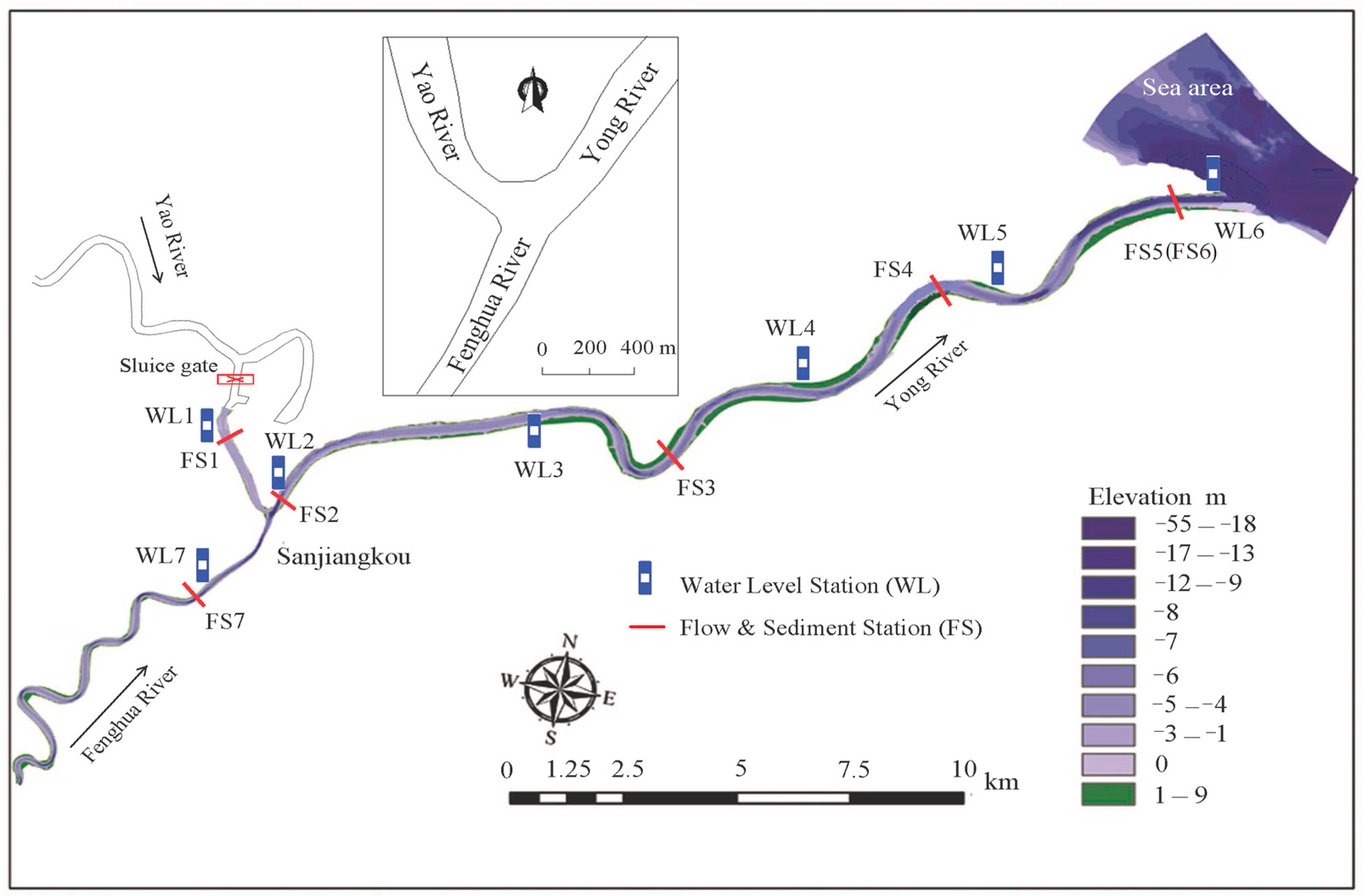
Figure 2.
Sketch of measurement arrangement at a cross-section.
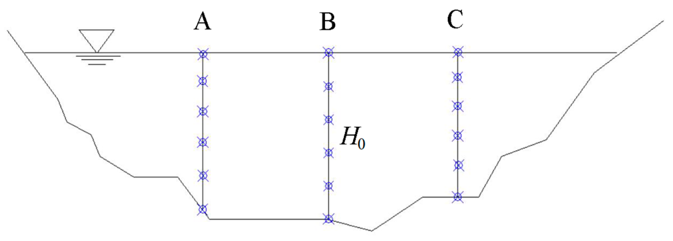
Figure 3.
Station FS5 (FS6), mean flow velocity vs. mean sediment concentration (V–S) relationship for spring and neap tides: (a) Spring tide; (b) Neap tide.
Figure 3.
Station FS5 (FS6), mean flow velocity vs. mean sediment concentration (V–S) relationship for spring and neap tides: (a) Spring tide; (b) Neap tide.
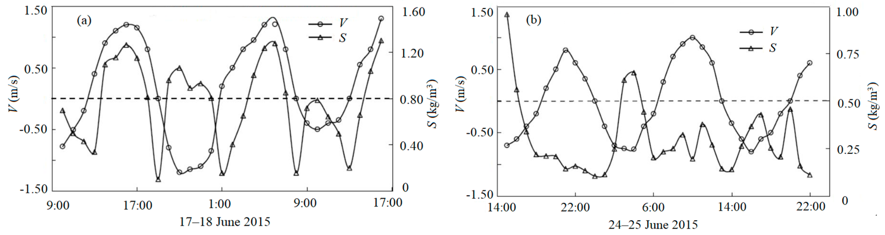
Figure 4.
Station FS2, V–S relationship for spring and neap tides: (a) Spring tide; (b) Neap tide.
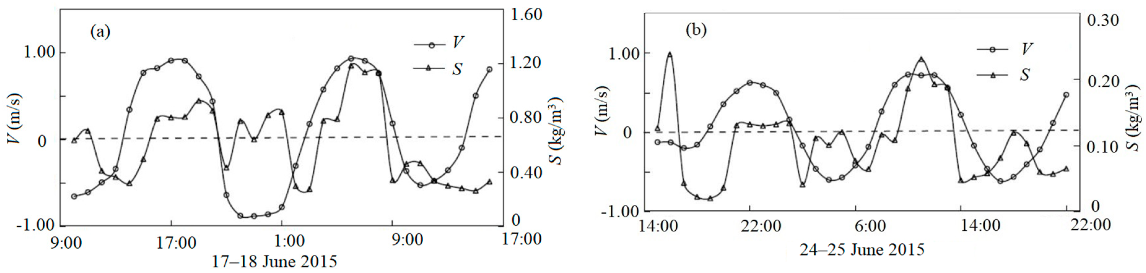
Figure 5.
Computational domain with cells.
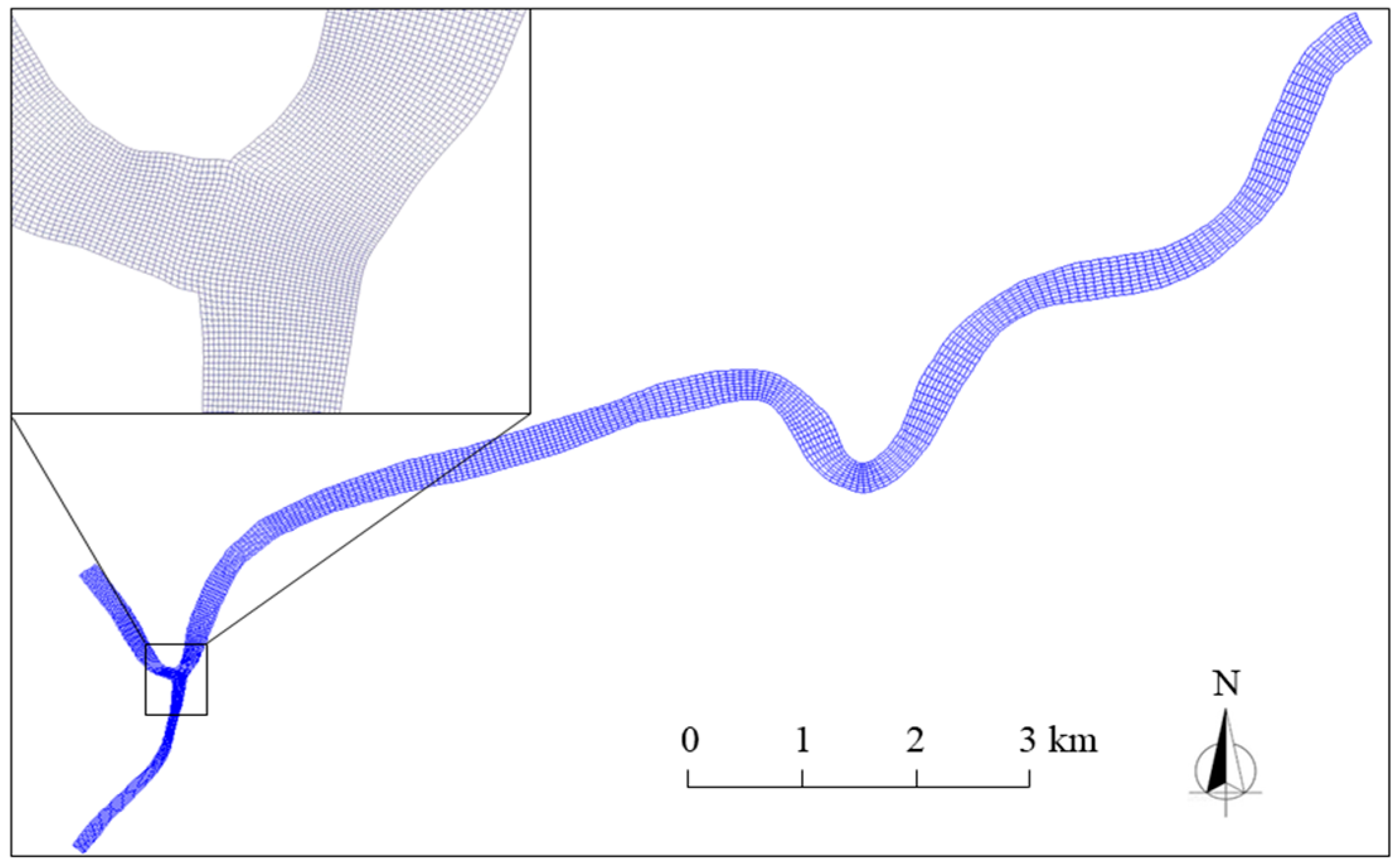
Figure 6.
Bathymetry of the study area with confluence.
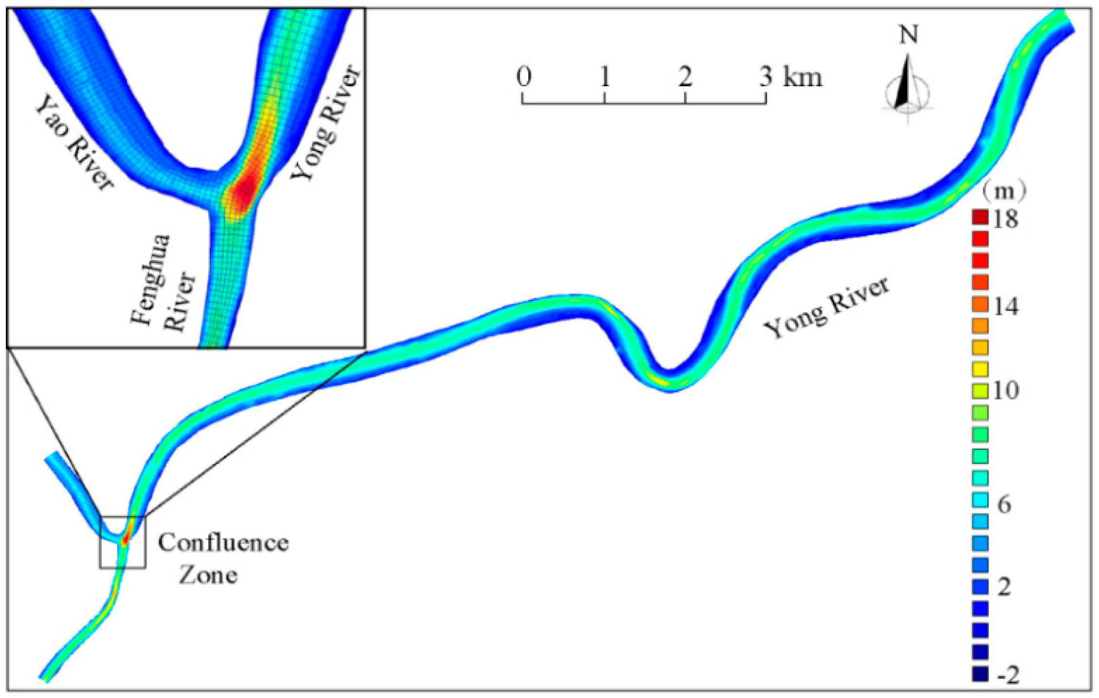
Figure 7.
Boundary conditions with measured data: (a) Flow discharge (Q); (b) Water stage (Z); (c) S.
Figure 7.
Boundary conditions with measured data: (a) Flow discharge (Q); (b) Water stage (Z); (c) S.
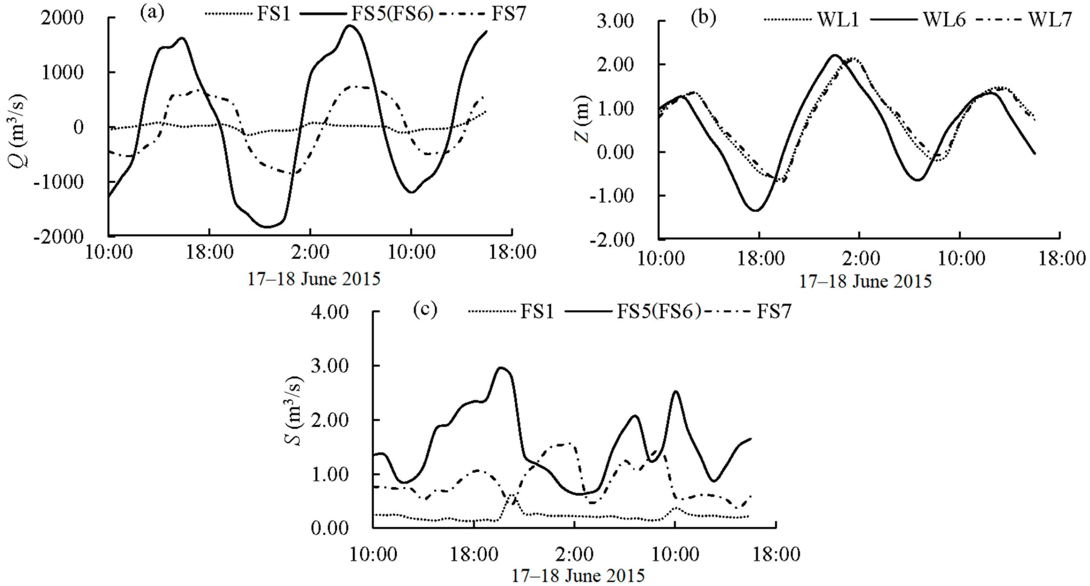
Figure 8.
Schematic diagram of the coupled flow and sediment calculations.

Figure 9.
Model calibration, numerical vs. field results at FS2 (spring tide, June 2015): (a) ; (b) S.
Figure 9.
Model calibration, numerical vs. field results at FS2 (spring tide, June 2015): (a) ; (b) S.

Figure 10.
Model calibration, numerical vs. field results at FS3 (spring tide, June 2015): (a) ; (b) S.
Figure 10.
Model calibration, numerical vs. field results at FS3 (spring tide, June 2015): (a) ; (b) S.

Figure 11.
Model calibration, numerical vs. field results at FS4 (spring tide, June 2015): (a) ; (b) S.
Figure 11.
Model calibration, numerical vs. field results at FS4 (spring tide, June 2015): (a) ; (b) S.

Figure 12.
Model validation, numerical results vs. field data at FS2 (neap tide, June 2015): (a) ; (b) S.
Figure 12.
Model validation, numerical results vs. field data at FS2 (neap tide, June 2015): (a) ; (b) S.

Figure 13.
Model validation, numerical results vs. field data at FS3 (neap tide, June 2015): (a) ; (b) S.
Figure 13.
Model validation, numerical results vs. field data at FS3 (neap tide, June 2015): (a) ; (b) S.

Figure 14.
Model validation, numerical results vs. field data at FS4 (neap tide, June 2015): (a) ; (b) S.
Figure 14.
Model validation, numerical results vs. field data at FS4 (neap tide, June 2015): (a) ; (b) S.
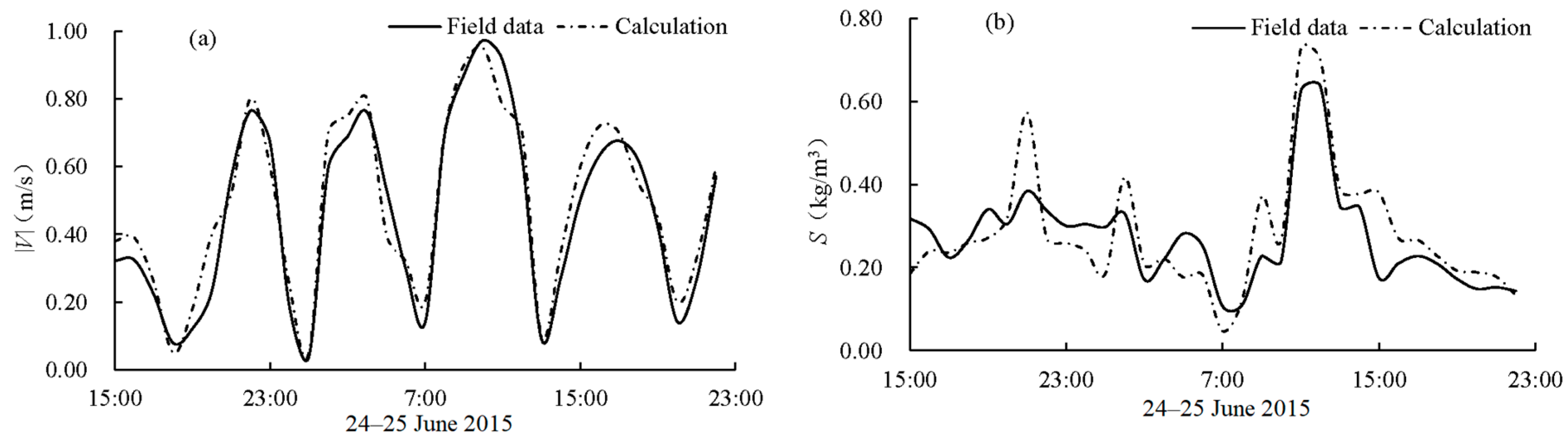
Figure 15.
Tidal flow fields during the second half of June 2015: (a) At the maximum flood tide; (b) At the maximum ebb tide.
Figure 15.
Tidal flow fields during the second half of June 2015: (a) At the maximum flood tide; (b) At the maximum ebb tide.
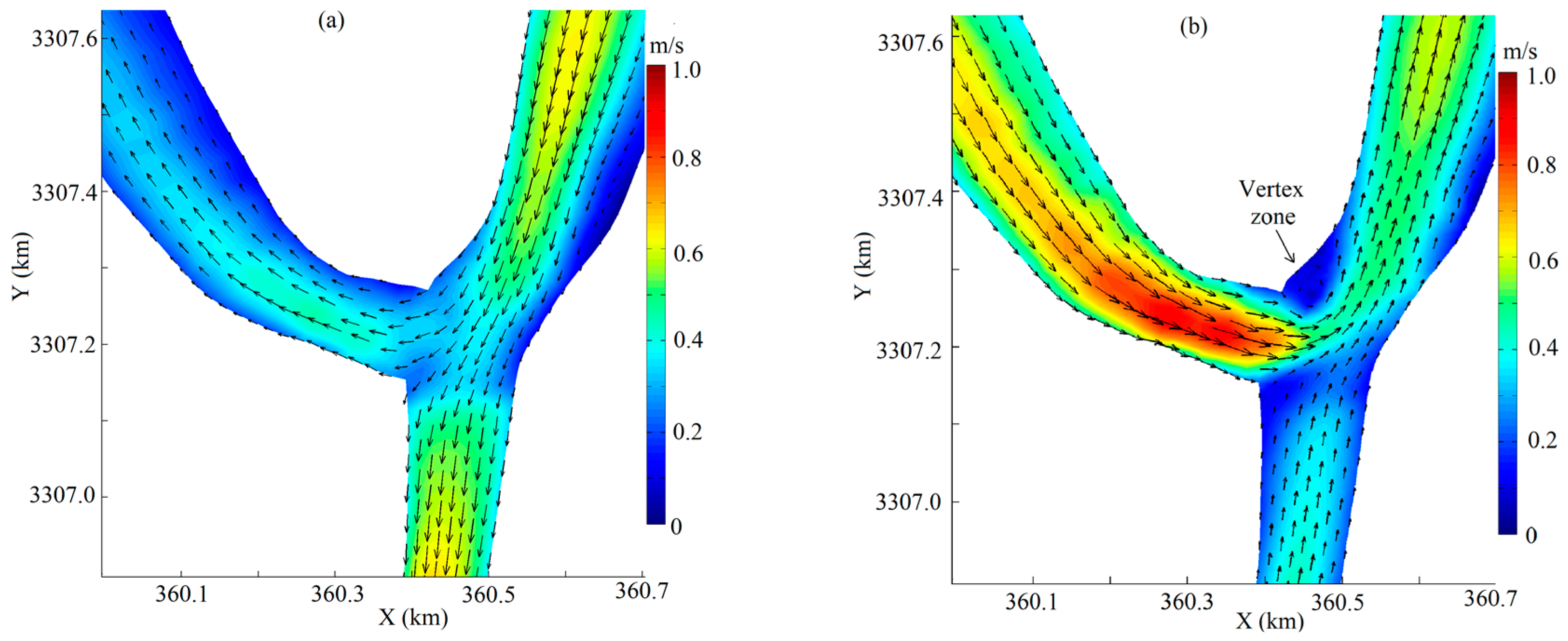
Figure 16.
Distributions of during the second half of June 2015: (a) At the maximum flood tide; (b) At the maximum ebb tide.
Figure 16.
Distributions of during the second half of June 2015: (a) At the maximum flood tide; (b) At the maximum ebb tide.

Figure 17.
Contours of the confluence in June 2015 (T = 0).
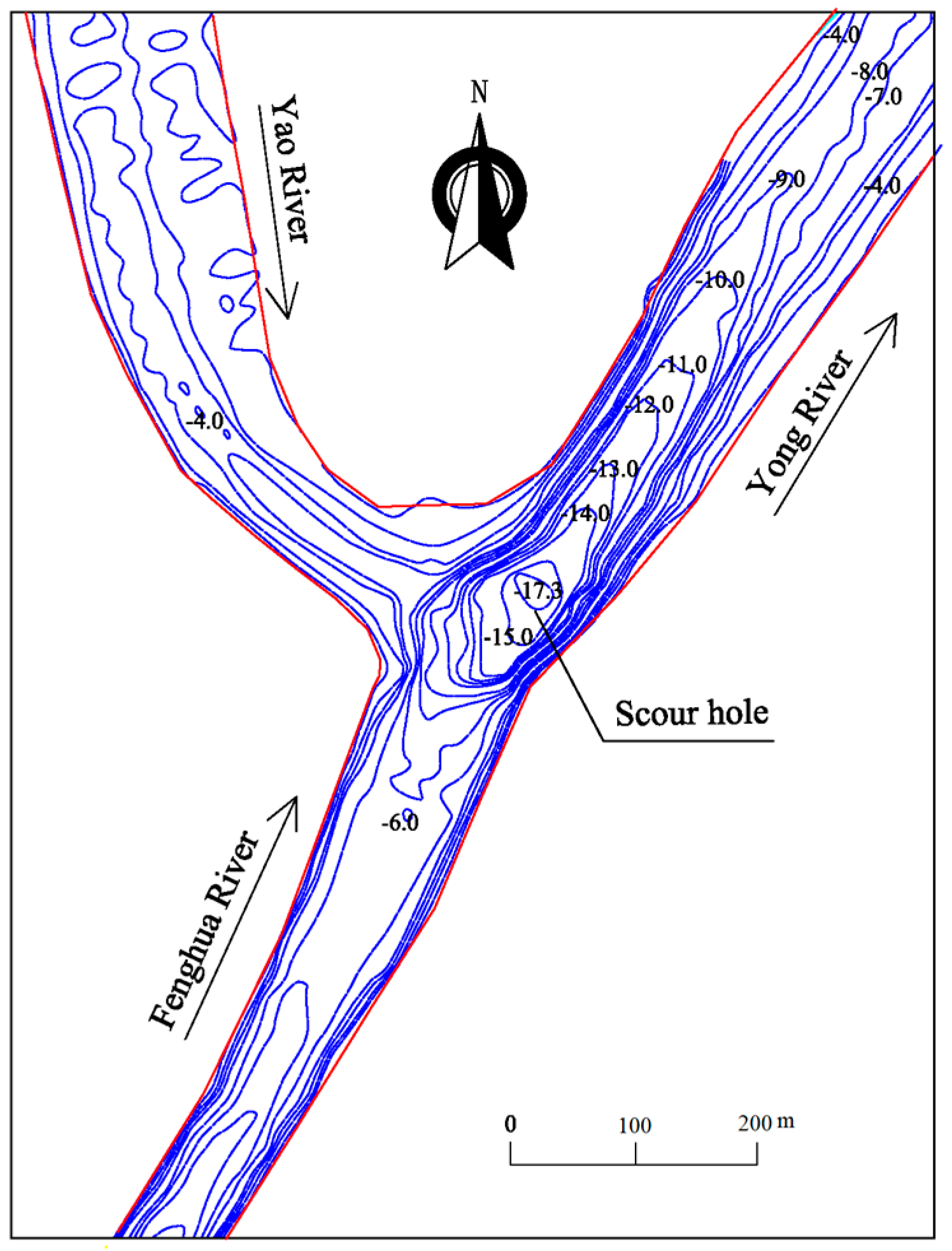
Figure 18.
River-bed morphology changes in the confluence: (a) T = 0; (b) T = 30 days; (c) T = 60 days; (d) T = 90 days; (e) T = 120 days; (f) T = 125 days.
Figure 18.
River-bed morphology changes in the confluence: (a) T = 0; (b) T = 30 days; (c) T = 60 days; (d) T = 90 days; (e) T = 120 days; (f) T = 125 days.
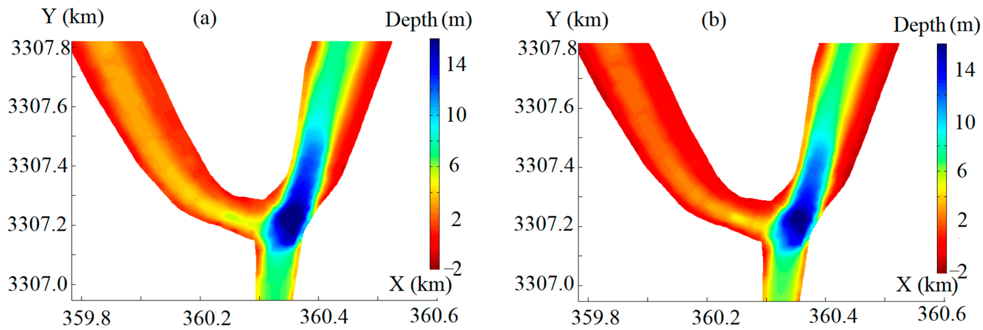

Figure 19.
Change in scour-hole depth in the confluence.
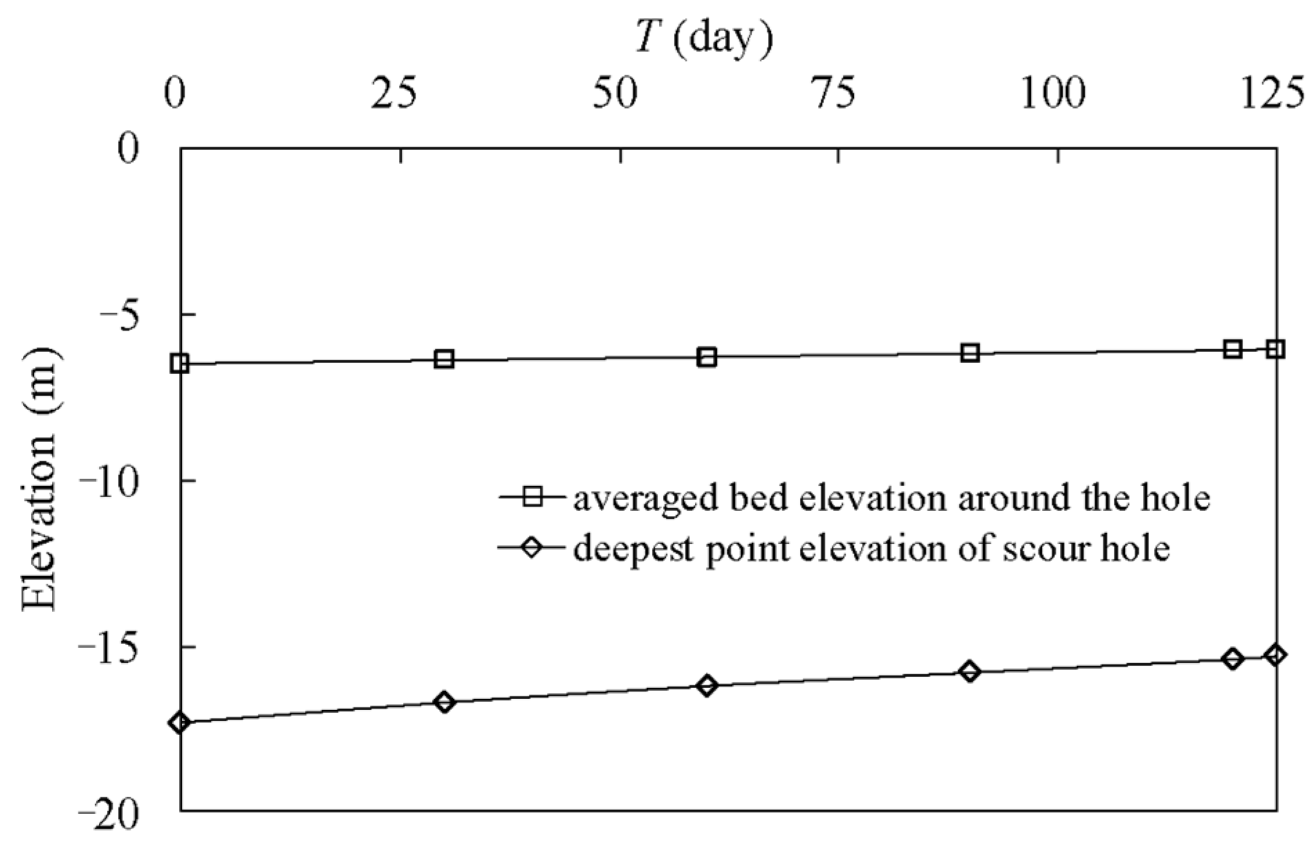
Figure 20.
Longitudinal bed-level changes in the confluence: (a) Distance along the river centerline (accounted from the lowest scour position); (b) Along the Yao River; (c) Along the Fenghua River; (d) Along the Yong River.
Figure 20.
Longitudinal bed-level changes in the confluence: (a) Distance along the river centerline (accounted from the lowest scour position); (b) Along the Yao River; (c) Along the Fenghua River; (d) Along the Yong River.


Table 1.
Distance of field measurement stations to the confluence.
| Water Level Station | WL1 | WL2 | WL3 | WL4 | WL5 | WL6 | WL7 |
| Distance to confluence (km) | 2.20 | 0.25 | 6.00 | 14.80 | 20.30 | 25.20 | 2.80 |
| Flow and Sediment Station | FS1 | FS2 | FS3 | FS4 | FS5 (FS6) | FS7 | |
| Distance to confluence (km) | 2.20 | 0.25 | 9.70 | 18.10 | 24.70 | 3.20 | |
Table 2.
Median grain sizes (D50) of suspended and bed load during the wet season (second half of June 2015).
Table 2.
Median grain sizes (D50) of suspended and bed load during the wet season (second half of June 2015).
| Station | Spring Tide, D50 (mm) | Neap Tide, D50 (mm) | ||
|---|---|---|---|---|
| Suspended Load | Bed Load | Suspended Load | Bed Load | |
| FS1 | 0.005 | 0.008 | 0.008 | 0.009 |
| FS2 | 0.007 | 0.013 | 0.007 | 0.016 |
| FS3 | 0.007 | 0.011 | 0.008 | 0.012 |
| FS4 | 0.008 | 0.019 | 0.006 | 0.020 |
| FS5 (FS6) | 0.008 | 0.011 | 0.007 | 0.011 |
| FS7 | 0.009 | 0.017 | 0.009 | 0.013 |
Table 3.
Time-averaged mean sediment concentration (S) values during the wet season (second half of June 2015).
Table 3.
Time-averaged mean sediment concentration (S) values during the wet season (second half of June 2015).
| Station | Spring Tide (kg/m3) | Neap Tide (kg/m3) | ||||
|---|---|---|---|---|---|---|
| Flood Tide | Ebb Tide | Semi-Diurnal Tide | Flood Tide | Ebb Tide | Semi-Diurnal Tide | |
| FS1 | - | - | 0.229 | - | - | 0.069 |
| FS2 | 0.780 | 0.541 | 0.677 | 0.121 | 0.089 | 0.106 |
| FS3 | 1.247 | 1.615 | 1.441 | 0.200 | 0.215 | 0.208 |
| FS4 | 2.341 | 2.117 | 2.207 | 0.232 | 0.318 | 0.282 |
| FS5 (FS6) | 1.673 | 1.476 | 1.578 | 0.314 | 0.214 | 0.265 |
| FS7 | 0.895 | 0.920 | 0.909 | 0.142 | 0.141 | 0.141 |
Table 4.
Parameter setting in the model.
| Parameter | Data Range | Source |
|---|---|---|
| (m/s) | 0.0005 | Measurements |
| (N/m2) | 0.06–0.10 | Equation (7) [39] |
| (N/m2) | 0.10–0.20 | Equation (8) [41] |
| M (kg/m2 s) | 0.0002–0.02 | Equation (8) [41] |
| (kg/m3) | 1600 | Measurements |
Table 5.
Definition of error parameters and their accepted ranges for calibration. NSE—Nash–Sutcliffe efficiency; PBIAS—percent bias.
Table 5.
Definition of error parameters and their accepted ranges for calibration. NSE—Nash–Sutcliffe efficiency; PBIAS—percent bias.
| Parameter | Optimal Value | Satisfactory | Equation |
|---|---|---|---|
| NSE | 1 | >0.5 | |
| R2 | 1 | >0.5 | |
| PBIAS | 0 | ±25% for flow rate | |
| ±55% for sediment |
Table 6.
Error estimations of model calibration (spring tide, June 2015).
| Parameter | FS2 | FS3 | FS4 | |||
|---|---|---|---|---|---|---|
| V (m/s) | S (kg/m3) | V (m/s) | S (kg/m3) | V (m/s) | S (kg/m3) | |
| NSE (>0.50) | 0.96 | 0.82 | 0.95 | 0.77 | 0.93 | 0.76 |
| R2 (0–1) | 0.97 | 0.80 | 0.95 | 0.79 | 0.94 | 0.78 |
| PBIAS (±25%) | 1.23 | −12.57 | 2.05 | −2.86 | 3.56 | 8.80 |
Table 7.
Error estimations of model validation (neap tide, June 2015).
| Parameter | FS2 | FS3 | FS4 | |||
|---|---|---|---|---|---|---|
| V (m/s) | S (kg/m3) | V (m/s) | S (kg/m3) | V (m/s) | S (kg/m3) | |
| NSE (>0.50) | 0.96 | 0.83 | 0.94 | 0.81 | 0.97 | 0.78 |
| R2 (0–1) | 0.95 | 0.84 | 0.93 | 0.79 | 0.96 | 0.75 |
| PBIAS (±25%) | 2.21 | −12.99 | 3.05 | −5.63 | 3.81 | 9.66 |
© 2018 by the authors. Licensee MDPI, Basel, Switzerland. This article is an open access article distributed under the terms and conditions of the Creative Commons Attribution (CC BY) license (http://creativecommons.org/licenses/by/4.0/).
Share and Cite
MDPI and ACS Style
Xie, Q.; Yang, J.; Lundström, S.; Dai, W. Understanding Morphodynamic Changes of a Tidal River Confluence through Field Measurements and Numerical Modeling. Water 2018, 10, 1424. https://doi.org/10.3390/w10101424
AMA Style
Xie Q, Yang J, Lundström S, Dai W. Understanding Morphodynamic Changes of a Tidal River Confluence through Field Measurements and Numerical Modeling. Water. 2018; 10(10):1424. https://doi.org/10.3390/w10101424
Chicago/Turabian StyleXie, Qiancheng, James Yang, Staffan Lundström, and Wenhong Dai. 2018. "Understanding Morphodynamic Changes of a Tidal River Confluence through Field Measurements and Numerical Modeling" Water 10, no. 10: 1424. https://doi.org/10.3390/w10101424
Note that from the first issue of 2016, this journal uses article numbers instead of page numbers. See further details here.