Model-Based Analysis of Increased Loads on the Performance of Activated Sludge and Waste Stabilization Ponds

Abstract

In a way to counter criticism on low cost-effective conventional activated sludge (AS) technology, waste stabilization ponds (WSPs) offer a valid alternative for wastewater treatment due to their simple and inexpensive operation. To evaluate this alternative with respect to its robustness and resilience capacity, we perform in silico experiments of different peak-load scenarios in two mathematical models representing the two systems. A systematic process of quality assurance for these virtual experiments is implemented, including sensitivity and identifiability analysis, with non-linear error propagation. Moreover, model calibration of a 210-day real experiment with 31 days of increased load was added to the evaluation. Generally speaking, increased-load scenarios run in silico showed that WSP systems are more resilient towards intermediate disturbances, hence, are suitable to treat not only municipal wastewater, but also industrial wastewater, such as poultry wastewater, and paperboard wastewater. However, when disturbances are extreme (over 7000 mg COD·L⁻¹), the common design of the natural system fails to perform better than AS. Besides, the application of sensitivity analysis reveals the most influential parameters on the performance of the two systems. In the AS system, parameters related to autotrophic bacteria have the highest influence on the dynamics of particulate organic matter, while nitrogen removal is largely driven by nitrification and denitrification. Conversely, with an insignificant contribution of heterotrophs, the nutrient removal in the pond system is mostly done by algal assimilation. Furthermore, this systematic model-based analysis proved to be a suitable means for investigating the maximum load of wastewater treatment systems, and from that avoiding environmental problems and high economic costs for cleaning surface waters after severe overload events.

1. Introduction

Conventional activated sludge (AS) systems, the most common application for sewage treatment, have recently been criticized due to their low cost-effectiveness, with high energy demand and limited recovery potential [1]. While the applicability of advanced technologies, such as membrane bioreactors, sand filtration, and aerobic granulation, is still being questioned in developing countries due to the barrier of affordability, waste stabilization ponds (WSPs) appeared to be an inexpensive, but effective, alternative. In fact, thanks to low cost and minimal operation and maintenance (O&M) requirements, WSPs are a major choice for wastewater treatment plants (WWTPs) in many countries, such as the US (>8000 installations), France (>2500 installations), and Germany (3000 installations) [2]. Until now, the practicability and feasibility of this alternative is mostly evaluated by system-specific data collection from different sources. These subjective comparisons resulted in relative general conclusions [3]. More importantly, a key criterion of these systems was missing, namely their resilience capacity to disruptions, which indicates the ability to adapt, endure, and recover from changing conditions [4,5]. Indeed, wastewater treatment plants (WWTPs) are normally long-lasting, with an expected lifespan of 60 to 70 years, hence the pre-selection assessment between different systems should account for possible future challenges to minimize additional expenses from reconstructions and adjustments [6,7].

Like any industrial sector, modeling in wastewater treatment plays an essential role in the system design and optimization. Especially, when investigating ill-defined natural systems, the ability to implement large and complex environmental models is of primary importance. Unlike parsimonious descriptive models, which have too little flexibility to accommodate changes in forcing factors [8], large environmental simulation models allow for analyzing system behavior and predicting future states of the systems [9]. These integrated mechanistic models can include complex interactions between hydrodynamic properties and biogeochemical cycles, hence favoring global extrapolation of their outputs. Therefore, mechanistic models are normally considered an excellent tool to perform in silico experiments, a virtual-world counterpart of real-world experiments [10]. By applying mathematical algorithms, the responses of the system to assumed changes in experimental conditions can be drawn without implementing real experiments, hence time and money can be saved [11].

Similar to the real experiments, intensive quality assurance (QA) guidelines for virtual simulation models have been established to support the decision making process [12]. Particularly, according to the precautionary principle in the field of water policy imposed by the EU Water Framework Directive, it is required to implement uncertainty assessment in integrated models [13]. Uncertainties can originate from different sources, i.e., model inputs, model structure, model parameters, and model software [12,14]. These prior uncertainties can then be quantified and propagated from model inputs to outputs via uncertainty analysis (UA). Besides, sensitivity analysis (SA) is another methodology for uncertainty assessment. This analysis studies how the uncertainty of model output can be allocated from different uncertainty sources of model inputs, which allows differentiating across parameters regarding their importance for the accuracy of the outcome [15]. According to Saltelli [16], uncertainty analysis and sensitivity analysis should be implemented in tandem.

In this study, the goal of this work was to investigate and compare the removal efficiency and resilience of two treatment systems, AS and WSP, via performing in silico experiments. To this end, two mechanistic models were built to simulate two specific configurations, i.e., the Wuhrmann process for AS systems, and conventional WSPs, including three compartments in series, an anaerobic (AP), a facultative (FP), and a maturation (MP) pond. Furthermore, to ensure the water management decisions, uncertainty assessment was carried out via different approaches. First, the most influential parameters and inputs were identified via a practical SA. Subsequently, these model parameters were calibrated by comparing the simulation outputs with the data observed from a 210-day experiment with 31 days of peak load scenario in the two systems. Eventually, we applied Monte Carlo simulations for nonlinear error propagation with the Latin Hypercube Sampling technique in several prospective scenarios of peak load to assess the robustness and recoverability of the two systems.

2. Materials and Methods

2.1. Experimental Setup

Lab-scale installations of the two systems were set up in triplicates in a temperature-controlled room with an air temperature of 21 (± 2) °C. Standard fluorescent lamps provided 16 h of illumination per day-night cycle. Artificial wastewater was prepared every 1.5 days and fed continuously to the systems, with an average flow of around three L d⁻¹, for 210 days. The recipe of the artificial wastewater was based on the OECD [17] guideline, resulting in a COD of 275 g O₂·m⁻³, total nitrogen (TN) of 40 g N·m⁻³, and total phosphorus (TP) of 7 g P·m⁻³. A specific configuration was selected for each treatment type, i.e., the Wuhrmann process for AS systems, and conventional WSPs, including three compartments in series, an anaerobic (AP), a facultative (FP), and a maturation (MP) pond. These configurations were chosen because of their basic, conventional, and common settings for removing organic matters and nutrients. The overview of the experimental setup of two treatment systems is illustrated in Figure S1 (Supplementary Material A) and its detailed description can be found in Ho, Van Echelpoel, Charalambous, Gordillo, Thas and Goethals [3]. To ensure the stability of the systems, their start-up period was maintained for 179 days, with samples being collected and analyzed two times per week. After the stabilization period, the peak load scenario was implemented in three phases. Standard artificial wastewater was fed to the systems for eight days of the first phase. Subsequently, the influent pollutant concentrations were tripled and then kept for five days of the second phase. The recovery of the systems was followed for the next 18 days with the initial wastewater in the third phase. The data collected from this peak load period were used for model calibration before the two models were applied in the scenario analysis.

2.2. Model Description

Two models representing the two systems were developed in the software, AQUASIM 2.1 [18]. Specifically, two compartments of an AS model were simulated within the completely mix module and connected via an advective link. The DO concentration was kept at 4 g O₂·m⁻³ in the first aerated compartment while there was no aeration supply in the second compartment. The AS model was developed, based on ASM2d, with 20 processes, including different microorganisms and microbial transformations. Sludge recirculation in the system was simulated as the biomass in the influent. A WSP model with three different compartments was simulated within the plug flow module, with each compartment containing different microorganisms, processes, and variables, hence increasing significantly the model complexity compared to the AS model. Within the plug-flow module, its assumption of a homogenous depth profile of variables is valid since the photosynthesis activity in facultative (FPs) and maturation ponds (MPs) can extend down to a depth of 20–30 cm, creating a homogenous aerobic condition in these oxidation ponds whose height is 20 cm [19,20]. Regarding the processes in the WSP model, following the Constructed Wetland Model No.1 of Langergraber, et al. [21], the anaerobic processes in the anaerobic compartment included the hydrolysis process of slowly biodegradable COD and the metabolism of anaerobic bacteria. FPs and MPs were modeled following the model of Sah, et al. [22], without pathogen removal and anaerobic bacteria due to relatively no sludge accumulation. The removal of phosphorus was assumed to have occurred mainly by chemical precipitation, hence, biological phosphorous removal processes were not considered. In addition, the gas exchange at the pond surface was included with reaeration of oxygen and ammonia volatilization. Light attenuation was accounted in the model to describe the exponential decrease of light intensity with depth according to Beer’s Law. More importantly, the cycle of day and night of light intensity are also included in the model to illustrate the fluctuation of algal photosynthesis and respiration activities. The interactions between all involved microbial groups are summarized in Supplementary Material B. The initial and influent conditions of the model variables are calculated and shown in Supplementary Material C. The details of stoichiometric matrix, kinetic rate expressions, and their values in the two models are shown in Supplementary Material D.

2.3. Parameter Estimation

2.3.1. Screening for Important Parameters

Sensitivity analysis (SA) evaluates the degree to which model inputs affect model output, and from that the universality and robustness of these parameters can be further investigated. The following technique of SA was proposed in Brun, et al. [23]. Firstly, the model is defined as described above. Subsequently, the prior uncertainties of model parameters and inputs (θ_j) are estimated, based on the literature [9,24,25]. The scale factors of model outputs, which are used to make the results for the various model endpoints comparable, are calculated, based on their mean concentrations in the pond system [26]. After these steps, Gaussian error propagation is applied to compute the sensitivity function, $s_{ij}$, for each state variable, y_i, against the changes of any parameter, θ_j, as shown in Equation (1):

$$s_{ij}=\frac{\Delta {\theta }_j}{s{c}_i}\frac{\partial y_i}{\partial {\theta }_j}$$

(1)

where ∆θ_j represents uncertainty ranges (∆) of the parameters and inputs were divided into three categories: Precisely known parameters (class 1), ∆θ_j = 5%; poorly known parameters (class 3), ∆θ_j = 50%; and moderately known parameters (class 2), ∆θ_j = 20%; sc_i is a scale factor of the state variable, y_i. The values of ∆θ_j and sc_i are listed in Supplementary Material E. The importance ranking was then determined based on the sensitivity measure, ${\delta }_j^{msqr}$, in Equation (2):

$${\delta }_j^{msqr}=\sqrt{\frac{1}{n}{\displaystyle \sum }_{i=1}^n{s}_{ij}^2}$$

(2)

A high ${\delta }_j^{msqr}$ means that the value of the parameter, θ_j, has an important influence on the simulation result while the sensitivity measure of zero indicates that the parameter has no effects on the model outputs.

2.3.2. Identifiability Assessment of Parameter Subsets

After the determination of ${\delta }_j^{msqr}$, the identifiability of the parameter subset, K, is estimated to avoid the compensation effect of the changes in the parameter values, θ_j, on the model output, y_i. This identifiability analysis of Brun, Reichert and Kunsch [23] is based on two different measures, collinearity index, $\gamma$, and determinant measure, $\rho$. The collinearity index represents the compensability of the parameter subset, K, which can be calculated as shown in Equation (3):

$${\gamma }_K=\frac{1}{mi{n}_{\Vert \beta =1\Vert }\Vert {\tilde{s}}_1{\beta }_1+\dots +{\tilde{s}}_K{\beta }_K\Vert }=\frac{1}{mi{n}_{\Vert \beta =1\Vert }\Vert \tilde{S}\beta \Vert }=\frac{1}{\sqrt{min(EV[{\tilde{S}}_K^T{\tilde{S}}_K])}}$$

(3)

where ${\tilde{S}}_K$ is an $n\times K$ submatrix of the normalized matrix, $\tilde{S}=\left\{{\tilde{s}}_{ij}\right\}$, with a normalized value of the sensitivity function, ${\tilde{s}}_{iK}=s_{iK}/\Vert s_{iK}\Vert$; $\beta ={\left({\beta }_1,\dots ,{\beta }_K\right)}^T$ is a vector of coefficient of the length, k, with the constraint, $\Vert \beta \Vert =1$; $EV$ is the eigenvalue of $[{\tilde{S}}_K^T{\tilde{S}}_K]$. ${\gamma }_K$ quantifies the degree of approximate linear dependence of the $s_{ij}$ of the parameters. A value of $\gamma$ over 10 indicates a poor identifiability of the parameter subsets [25]. The second criterion, the determinant measure, $\rho$, is defined as shown in Equation (4):

$${\rho }_K=det{\left({\tilde{S}}_K^T{\tilde{S}}_K\right)}^{1/2K}$$

(4)

The determinant measure, $\rho$, is proposed by Weijers and Vanrolleghem [27], which combines the information provided by ${\delta }_j^{msqr}$ and $\gamma$. A high value of ${\rho }_K$ indicates a low value of $\gamma$ and a high value of ${\delta }_j^{msqr}$, hence a good “conditional identifiability” of a parameter subset [26].

2.3.3. Model Calibration

After SA and IA, a subset of identifiable and influential parameters is chosen for calibration with the data collected from the shock-load experiment. Generally, to objectify the calibration process, a function representing the agreement between the model and data is defined to demonstrate the desire to fit the model to the data [28]. In this case, the weighted sum of squares (WSS) of the residuals is minimized, from which selected parameters are calibrated using the simplex algorithm in the AQUASIM 2.1 software [18]. To calculate the WSS, each residual is divided by a scale factor (sc_i) of the corresponding variable, y_i, from that the residuals become non-dimensional as sc_i and the model output have the same dimension [25].

$$WSS\left({\theta }_j\right)={\displaystyle \sum }_{i=1}^n{\left(\frac{y_{meas,i}-y_i\left({\theta }_j\right)}{s{c}_i}\right)}^2$$

(5)

In this equation, $y_{meas,i}$ is the i-th measurement, $y_i\left({\theta }_j\right)$ is the calculated value of the model output corresponding to the i-th measurement and evaluated at the time and location of this measurement, and n is the number of data points.

2.4. Scenario Analysis

To evaluate the impact of increased loads on the performance of the two systems, several prospective scenarios were simulated using the UNCSIM package [29]. These theoretical simplified scenarios include quantitative changes in the pollutant concentrations, which are expected to occur in real WWTPs. According to Joseph [30], four baseline scenarios representing two intermediate and two extreme conditions are a good starting point for the development of further policy scenarios. As such, we implemented four scenarios of different wastewater strengths, i.e., 2, 5, 10, and 25 times higher than the standard OECD domestic wastewater. These scenarios allow investigation of the increased load threshold of which the two systems can still be able to recover to the initial conditions, hence, the conclusion of their robustness and recoverability can be withdrawn. More importantly, to ascertain the water management decision process, the Monte Carlo simulation was applied to compute the model output uncertainty as a result of the prior uncertainty of model parameters and inputs (listed in Supplementary Material E). 500 sets of samples were generated using the Latin Hypercube Sampling (LHS) technique, which provides a sufficient coverage of the parameter space with optimal computation time [31]. Scenarios caused by hydraulic overloading were not considered in this study as their practical solution is normally based on flow management with the manipulation of the proportion of by-passed water flow and the design of control structure.

3. Results

3.1. Sensitivity Analysis

Sensitivity analysis (SA) is designed as a tool to identify the most influential model parameters for the variability of the state variables. For the overparameterized models, SA is considered very useful as the model output is often strongly influenced by few key inputs [16]. In this case study, we investigate particularly the degree to which model inputs affected two groups of model output, i.e., organic matter and nutrient removal.

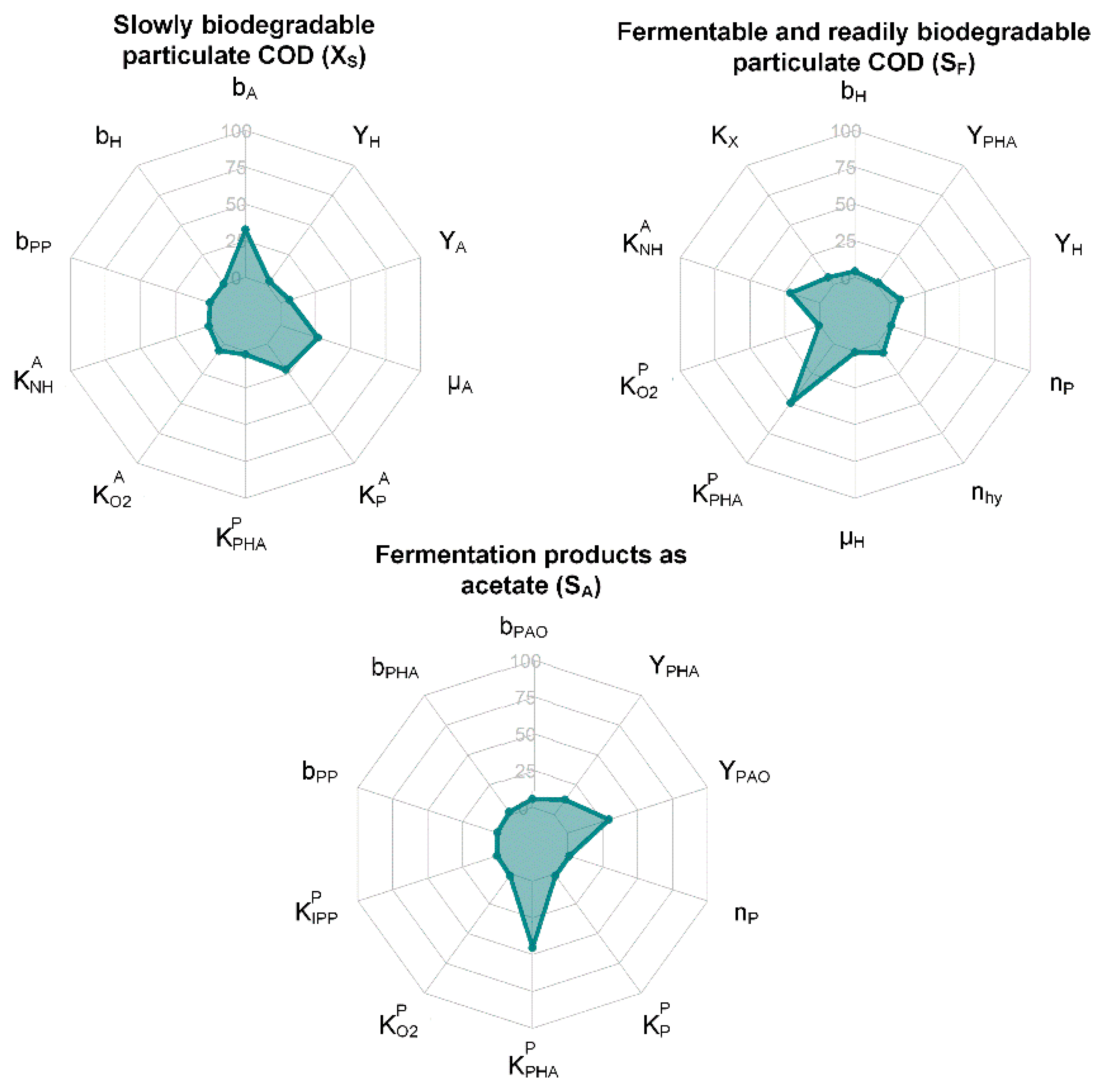
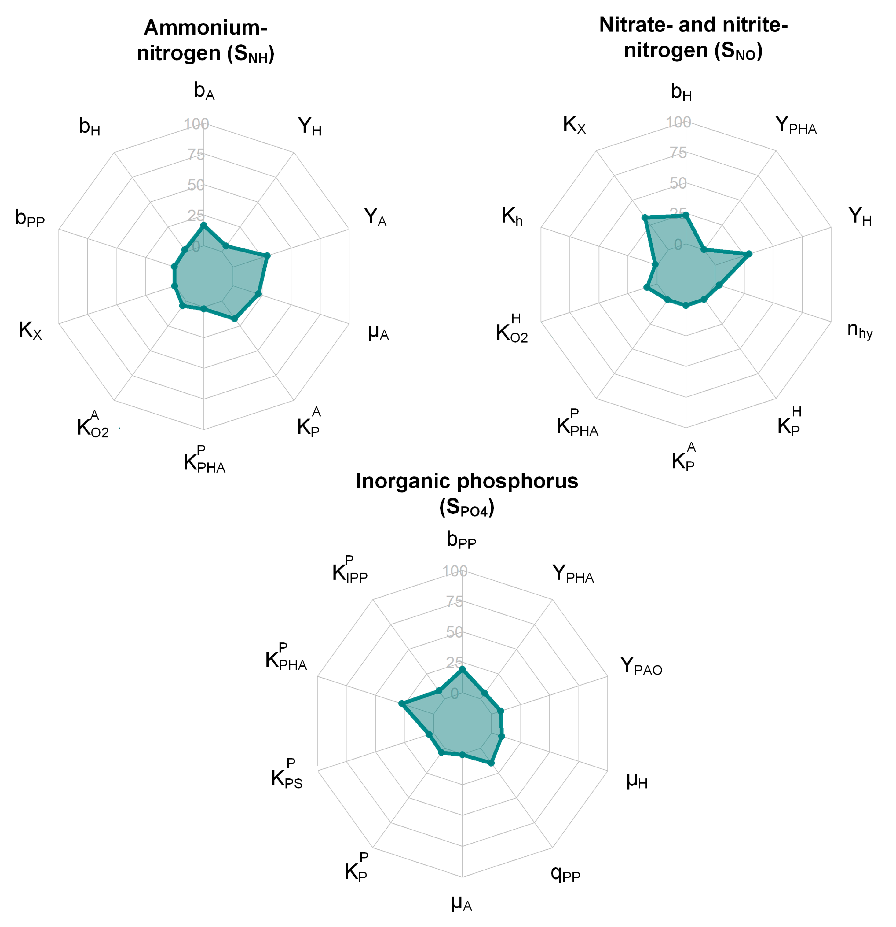
3.1.1. Activated Sludge Model

The Most Influential Parameters for Organic Matter Removal

Organic matter (OM) content in wastewater can be measured via COD, which includes slowly biodegradable particulate COD (X_S), fermentable and readily biodegradable soluble COD (S_F), fermentation products as acetate (S_A), inert soluble, and particulate COD (S_I and X_I), and COD from bacterial biomass. However, not all of these components are of equal importance [32]. Particularly, the COD fraction from microorganisms and the inert COD are also not in our interest because of the marginal variation of their values. To identify the most influential model parameters for the first three COD fractions, i.e., X_S, S_F, and S_A, we calculate the proportions of sensitivity function ($s_{ij}$) for each of the three state variables against the changes of each parameter, θ_j, over the total sum of sensitivity measures. As seen in Figure 1, the most significant parameters influencing the concentration of X_S is related to autotrophic bacteria, i.e., b_A, µ_A, ${\mathrm{K}}_{\mathrm{P}}^{\mathrm{A}},{\mathrm{K}}_{\mathrm{O}2}^{\mathrm{A}}$, and Y_A. These parameters are responsible for more than 90% of the total variance of the concentration of X_S. The main degradation process of the particulate COD is hydrolysis, which is sensitive to the availability of dissolved oxygen in the system. On the one hand, the presence of dissolved oxygen is needed for the aerobic hydrolysis, but on the other hand, the prevalence of O₂ inhibits the process rate of hydrolysis under anoxic and anaerobic conditions. Therefore, the parameters related to autotrophs, which are one of the main oxygen consumers, can affect considerably the removal of particulate COD. The influence of oxygen on OM removal in the AS system is also indicated in the case of S_F in which the saturation/inhibition coefficient of heterotrophs for oxygen (${\mathrm{K}}_{\mathrm{O}2}^{\mathrm{H}}$) explains 20% of its total variance. Also noteworthy is the substantial contribution of saturation coefficient for PHA storage in PAOs (${\mathrm{K}}_{\mathrm{PHA}}^{\mathrm{P}}$) in the total variances of soluble COD, i.e., around 50% for both S_F and S_A. The high importance ranking of this kinetic parameter is also recorded in several studies on the parameter identification of biological wastewater model in the literature [26,33,34].

The Most Influential Parameters for Nutrient Removal

Nutrient content in municipal wastewater mainly includes two fractions of nitrogen and phosphorus. Particularly, the total nitrogen concentration contains particulate and soluble Kjeldahl nitrogen (TKN), and nitrate- and nitrite-nitrogen (S_NO) [32]. Particulate Kjeldahl nitrogen, as the sum of nitrogen bound to all organic particulate fractions, is not investigated due to its marginal values compared to the value of soluble Kjeldahl nitrogen, which is dominated by ammonium-nitrogen (S_NH), likewise with particulate phosphorus. As such, the most influential model parameters for nutrient removal represented by the variance of S_NH, S_NO, and S_PO4 are shown in Figure 2. Regarding the first state variable, it appears that nitrification is a main process of ammonium removal in the AS system, which is indicated via the growth of ammonium and nitrite oxidizers as Y_A, µ_A, and ${\mathrm{K}}_{\mathrm{P}}^{\mathrm{A}}$ and are responsible for up to 70% of the total variance. On the other hand, parameters related to denitrification, i.e., ${\mathrm{Y}}_{\mathrm{H}},{\mathrm{K}}_{\mathrm{P}}^{\mathrm{A}}$, and b_H, contributes around 50% of the total variance of S_NO, indicating the significant role of denitrification in nitrite and nitrate removals. Besides, hydrolysis also appears to be important to the variability of S_NO, which can be explained by the fact that, apart from the influence, hydrolysis is the main source of S_F, the only electron donor of the denitrification process in this case. As such, the changes in values of K_h, K_X, and n_hy can affect considerably the availability of S_NO in the AS systems. Note that the process of bacterial assimilation plays an insignificant role in both nitrogen and phosphorus removal. The latter process is mainly carried out via PAOs, the group of organisms that have the ability to accumulate phosphorus in excess of normal metabolic requirements [35]. As such, from the radar graph, most of the influential parameters for S_PO4 are related to the metabolic process of PAO.

The Most Important Parameters Driving Model Outputs

After calculating the $s_{ij}$, the further step of SA, following the procedure of Brun, Reichert and Kunsch [23], is the computation of importance rankings of the parameters (${\delta }^{msqr}$) to detect the parameters driving the variability most in the model outputs. Having the highest influence on model outputs and significant contribution to model uncertainty, 20 parameters with the highest value of ${\delta }^{msqr}$ are presented in Table S16 (Supplementary Material G). The ranking shows that the PAO-related parameters, accounting for eight out of the 20 most important parameters, drive the variability in most of the model outputs, which is in line with previous studies on parameter identifiability of ASM2d, i.e., Brun, Kuhni, Siegrist, Gujer and Reichert [26], Ferrero, Chai, Diez, Amrani and Lie [33], and Liau, Shoji, Ong, Chua, Yeoh and Ho [34]. However, in contrast to the low importance of autotroph-related parameters in these enhanced biological phosphorus removal (EBPR) systems, high sensitivity of the model output toward nitrification is indicated via the position of µ_A and Y_A in this post-denitrification system.

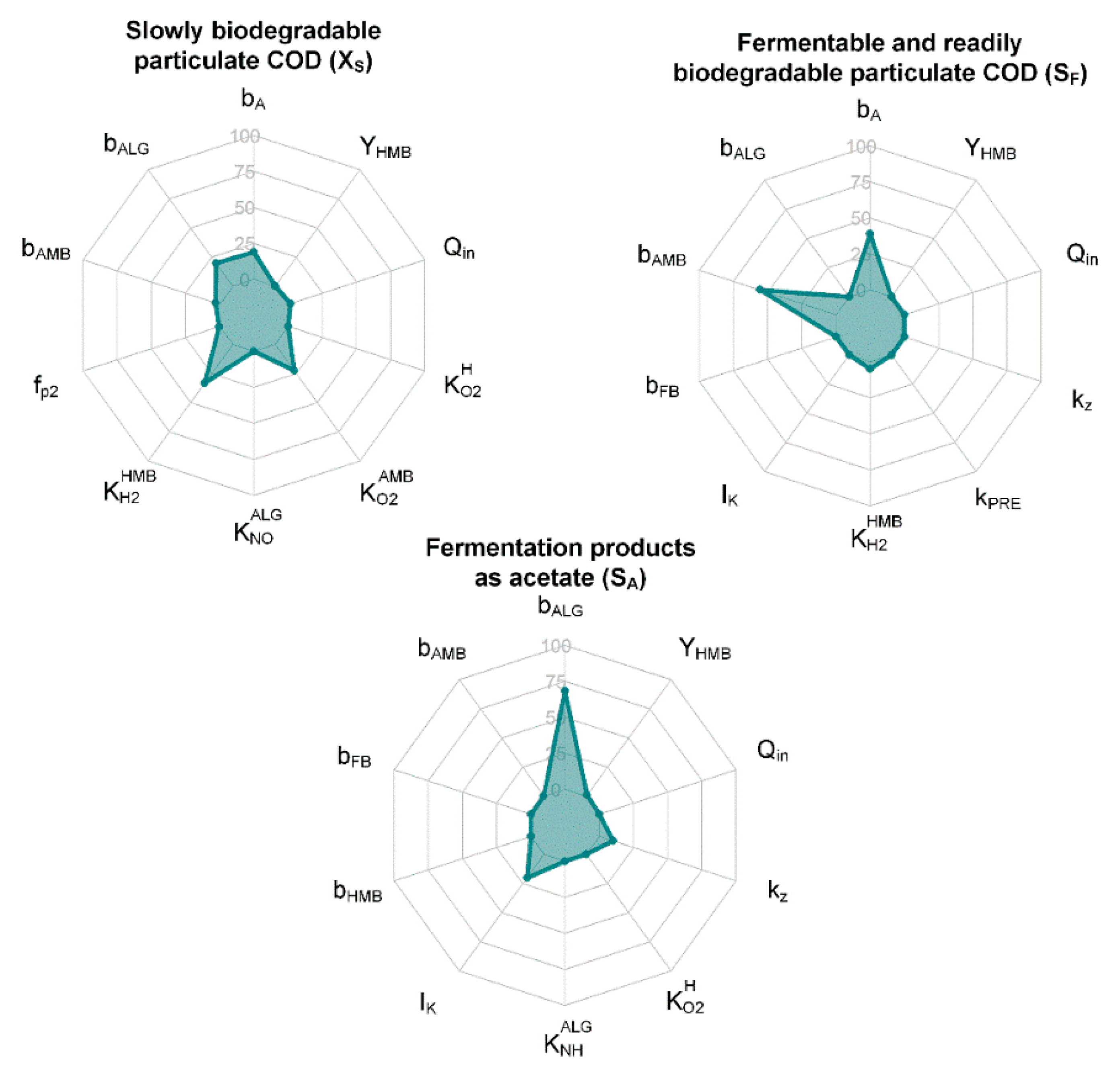
3.1.2. Waste Stabilization Pond Model

The Most Influential Parameters for Organic Matter Removal

As can be seen from Figure 3, the following parameters were found to have a significant impact on the variability of X_S (listed in the decreasing order of importance): ${\mathrm{K}}_{\mathrm{H}2}^{\mathrm{HMB}},{\mathrm{K}}_{\mathrm{O}2}^{\mathrm{AMB}}$, b_A, and b_ALG. The first two coefficients suggest the important role of methanogenic bacteria in anaerobic digestion, which is the main removal process of X_S. While the low concentration of H₂ as the electron donor in pond systems is the limiting factor of the growth of HMB, a very low value of ${\mathrm{K}}_{\mathrm{O}2}^{\mathrm{AMB}}$, 0.0002 g O₂.m⁻³, indicates the high sensitivity of this bacteria toward O₂. The influence of the oxygen level in the system on OM removal is displayed in the presence of the decay rate of algae, the main oxygen producer, and autotrophs, the main oxygen consumer, whose changes also significantly affect the total variance of S_F and S_A. In fact, as algal photosynthesis is the only source of O₂ for heterotrophs to degrade S_A in the FPs and MPs, the decay rate of algae appears to be a main contributor to its total variability, together with other photosynthesis-related parameters, including the light extinction coefficient and light saturation constant. Also noteworthy is that AMB proves to have a more important role in removing S_F compared to HMB in anaerobic digestion as b_AMB contributes to 35% of the total variance of S_F, which can be explained by the fact that their electron donor, S_A, is more available than H₂.

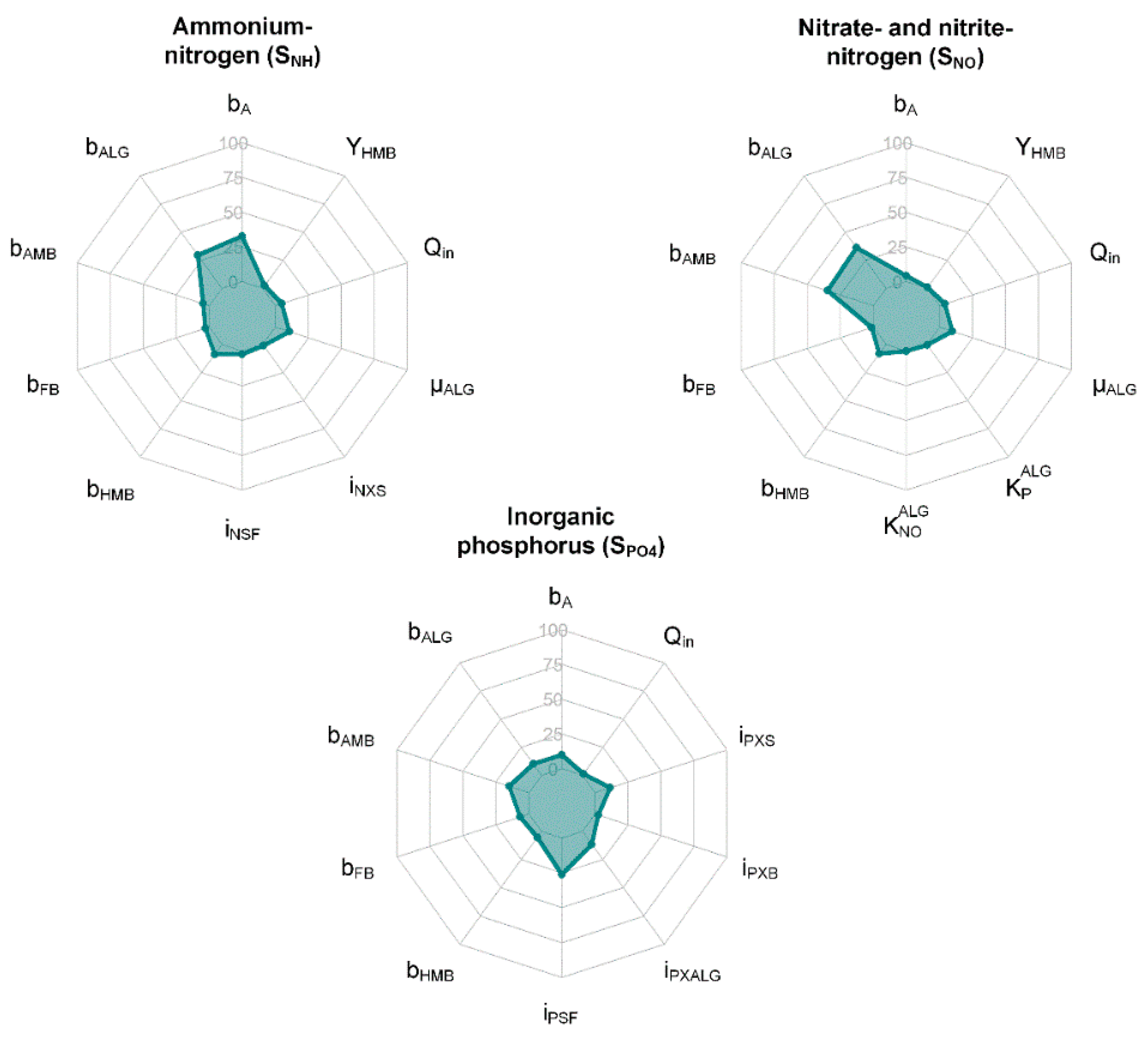
The Most Influential Parameters for Nutrient Removal

As shown in Figure 4, the variability of nutrient variables was affected significantly by the rate of growth and decay of algae. Particularly, around 40% of the total variance of S_NH within the pond systems was caused by the metabolisms of algae, suggesting the important role of both algal assimilation and oxygen supply to nitrification of autotrophs in ammonium removal. While the decay of bacteria is a minor source of S_NH in the system, which is reflected by a small contribution percentage of decay rates of other bacteria, these processes contributed around 25% of the variability of S_NO and S_PO4. These results suggest that as a result of long hydraulic retention time, bacteria and algae in the pond systems can release nutrients into the water body via their decay process. This reflects on the list of influential parameters for S_PO4 containing high contribution percentage of phosphorus fraction in different components, which are related to the decay process of algae and different bacteria. In contrast to this contribution, the disappearance of parameters related to heterotrophic bacteria in nitrogen removal and the chemical precipitation process in phosphorus removal suggest their marginal role in pond systems.

The Most Important Parameters Driving Model Outputs

Based on the values of ${\delta }^{msqr}$, the 20 parameters contributing the most on the variability of the outputs and uncertainty of the WSP model are presented in Table S17 (Supplementary material G). Noticeably, the five highest ranking parameters driving the most output variance are the parameters that can affect the process rate of the algal photosynthesis. Indeed, besides µ_ALG, light availability appears to be highly influential on the performance of both algal activity and the pond system. High sensitivity of the model output toward other physical parameters representing the temperature influence, i.e., θ_Tw and T_w, is also observed. Indeed, temperature and other climatic conditions, such as solar radiation, are very important to the pond performance [36]. Also noteworthy is the high importance of the flow rate on the performance of the WSP system. Finally, two stoichiometric parameters (Y_FB and Y_HMB) among the top ten parameters suggest the important role of anaerobic bacteria in the first compartment of the WSP system.

3.2. Identifiability Analysis

3.2.1. Activated Sludge Model

The possibility of compensating a change in model output caused by a change of one parameter by the others is evaluated via two measures, i.e., the collinearity index, $\gamma$, and determinant measure, $\rho$. The top 20 parameters of importance ranked in Table S12 are divided into three functional groups, including hydrolysis, autotroph, and PAO-related process, to investigate their correlations via $\gamma$ and $\rho$ (see

Table 1. Collinearity index ($\gamma$) and determinant measure ($\rho$) of selected parameters subsets. Based on their function, the parameters are categorized into different process groups, i.e., hydrolysis, autotroph, and PAO-related processes. The subset in bold is selected for parameter estimation based on values of $\gamma$ and $\rho$.

Group	Set Size	γ	ρ	Parameters
Hydrolysis	3	1.58	16.11	YH, µH, ${\mathrm{K}}_{\mathrm{F}}^{\mathrm{H}}$
	4	1.91	13.48	YH, µH, ${\mathrm{K}}_{\mathrm{F}}^{\mathrm{H}}$, Kh
	4	1.71	13.44	YH, µH, ${\mathrm{K}}_{\mathrm{F}}^{\mathrm{H}}$, bH
	5	2.77	11.45	YH, µH, ${\mathrm{K}}_{\mathrm{F}}^{\mathrm{H}}$, Kh, bH
Autotrophic	2	3.01	15.52	µA, YA
	3	8.12	6.43	µA, YA, bA
	3	3.73	7.55	µA, YA, ${\mathrm{K}}_{\mathrm{O}2}^{\mathrm{A}}$
PAO	4	4.98	24.92	qPP, YPAO, bPAO, YPHA
	5	5.24	18.65	qPP, YPAO, bPAO, YPHA, bPHA
	5	9.21	15.35	qPP, YPAO, bPAO, YPHA, ${\mathrm{K}}_{\mathrm{PHA}}^{\mathrm{P}}$
	6	9.34	12.98	qPP, YPAO, bPAO, YPHA, ${\mathrm{K}}_{\mathrm{PHA}}^{\mathrm{P}}$, bPHA
	6	9.22	11.23	qPP, YPAO, bPAO, YPHA, ${\mathrm{K}}_{\mathrm{PHA}}^{\mathrm{P}}$, bPP
Combination	10	8.39	14.43	qPP, YPAO, bPAO, YPHA, YH, µH, $K_F^H$, µA, YA, bH
	10	8.74	12.81	qPP, YPAO, bPAO, YPHA, YH, µH, ${\mathrm{K}}_{\mathrm{F}}^{\mathrm{H}}$, µA, YA, bPP
	10	10.68	12.67	qPP, YPAO, bPAO, YPHA, YH, µH, ${\mathrm{K}}_{\mathrm{F}}^{\mathrm{H}}$, µA, YA, ${\mathrm{K}}_{\mathrm{PHA}}^{\mathrm{P}}$
	11	10.86	10.86	qPP, YPAO, bPAO, YPHA, YH, µH, ${\mathrm{K}}_{\mathrm{F}}^{\mathrm{H}}$, µA, YA, ${\mathrm{K}}_{\mathrm{PHA}}^{\mathrm{P}}$, bPP
	11	11.01	12.10	qPP, YPAO, bPAO, YPHA, YH, µH, ${\mathrm{K}}_{\mathrm{F}}^{\mathrm{H}}$, µA, YA, ${\mathrm{K}}_{\mathrm{PHA}}^{\mathrm{P}}$, Kh

). Turning to parameters related to PAO, it is noticeable that the top four parameters show a relatively small $\gamma$ of 4.98 and a high $\rho$ of 24.92, which makes them identifiable from the available data. On the other hand, we observe a strong interdependence between the PHA saturation coefficient (${\mathrm{K}}_{\mathrm{PHA}}^{\mathrm{P}}$) and these four parameters, which could be a result of the high influence of ${\mathrm{K}}_{\mathrm{PHA}}^{\mathrm{P}}$ on both the growth and polyphosphate storage processes of PAO [37]. A strong correlation between µ_A and b_A is recorded, which infers the simultaneous estimation of these two parameters is likely to fail. Considering the determinant measure, a higher value in the PAO group indicates its more influential role on the system performance compared to the other two groups. After inspecting the correlation among parameters of all subsets, γ and ρ are calculated for the possible subsets of size 10 and 11. They can be combined by four hydrolysis parameters, three linked to autotrophs, and five PAO-related parameters. Noticeably, most of the subsets with size 11 have $\gamma$ higher than the threshold of 10 while their value range of $\rho$ fluctuates between 10 and 13. Hence, after assessing all of the combination group of size 10, the subset in bold is selected based on its low value of γ and high value of ρ compared to other subsets.

3.2.2. Waste Stabilization Pond Model

Table 2. Collinearity index ($\gamma$) and ($\rho$) of selected parameters subsets. Based on their function, the parameters are categorized into different process groups, i.e., physical, anaerobic, algal activity, autotrophic, and heterotrophic processes. The subset in bold is selected for parameter estimation based on values of $\gamma$ and $\rho .$

Group	Set Size	γ	ρ	Parameters
Physical	3	2.15	18.92	IK, θTw, kz
	4	2.16	16.66	IK, θTw, kz, Tw
	4	2.16	17.05	IK, θTw, kz, Qin
Anaerobic	2	1.63	9.93	YFB, YHMB
	3	3.51	5.56	YFB, YHMB, µHMB
	3	1.96	4.63	YFB, YHMB, µFB
Algal activity	2	1.02	11.21	µALG, pH
	2	2.02	8.51	µALG, bALG
	3	1.26	8.40	µALG, pH, bALG
Autotrophic	2	1.26	4.46	YA, bA
	2	1.61	2.95	YA, iNXS
	3	1.68	2.69	YA, bA, iNXS
Heterotrophic	2	1.30	10.1	fp2, YH
	3	1.56	6.19	fp2, YH, nH
	3	1.32	6.43	fp2, YH, ${\mathrm{K}}_{\mathrm{O}2}^{\mathrm{H}}$
	3	1.36	5.28	fp2, YH, ${\mathrm{K}}_{\mathrm{A}}^{\mathrm{H}}$
Combination	12	3.83	8.66	IK, θTw, kz, YFB, YHMB, µALG, pH, YA, bA, fp2, YH, Qin
	12	3.91	8.58	IK, θTw, kz, YFB, YHMB, µALG, pH, YA, bA, fp2, YH, Tw
	12	4.62	7.34	IK, θTw, kz, YFB, YHMB, µALG, pH, YA, bA, fp2, YH, µHMB
	13	3.92	8.70	IK, θTw, kz, YFB, YHMB, µALG, pH, YA, bA, fp2, YH, Tw, Qin
	13	4.04	6.28	IK, θTw, kz, YFB, YHMB, µALG, pH, YA, bA, fp2, YH, µFB, nH

shows the collinearity index ($\gamma$) and determinant measure ($\rho$) of the top 20 influential parameters, which are divided into five functional groups, i.e., physical, anaerobic, algal activity, autotrophic, and heterotrophic processes, to investigate their correlations. As seen in Table 2, the value range of former criterion stays low, between 1 and 5, which suggests that the proposed threshold of Brun, Kuhni, Siegrist, Gujer and Reichert [26] can be irrelevant for classifying non-identifiable parameters in this case. As this subjective threshold can be varied in different case studies, the combination with another criterion, such as the determinant measure, is necessary [38]. According to the value of $\rho$, the physical and algal-related parameters appear to have a high influence on the model outputs while parameters linked to autotrophic bacteria can generate less impact on the performance of the pond system. It is noticeable that when the subset size increases in all of the groups, except for the first group, there is a significant drop of the value of $\rho$. Hence, the chosen combined subsets have the size of 12 and 13, including four physical parameters and two parameters of each of other groups. From the obtained results, it is revealed that there is a small difference in the value of $\gamma$ and $\rho$ between the combined subsets of size 12 and 13. Noticeably, the higher value of the second criterion belongs to subsets that include more physical parameters. As such, with the highest value of $\rho$, the parameter subset of size 13 in bold, including all five physical parameters, is selected for calibration.

3.3. Model Calibration

After the establishment of a subset of 10 selected parameters for the AS model, an automatic calibration was performed on the basis of the collected data until the convergence in simplex algorithm is achieved in AQUASIM [18]. The original and calibrated results are shown in

Table 3. Original and calibrated values of the selected parameters in the AS model.

Parameters	Unit	ASM 2d	Calibrated Values	Δ (%)
bH	d−1	0.4	0.22	−45.27
bPAO	d−1	0.2	0.24	18.51
${\mathrm{K}}_{\mathrm{F}}^{\mathrm{H}}$	g COD· m−3	3	2.86	−4.69
µA	d−1	1	1.09	8.83
µH	d−1	6	6.15	2.55
qPP	g XPP·g−1 XPAO d−1	1.5	1.59	5.80
YA	g COD·g−1 N	0.24	0.28	15.19
YH	g COD·g−1 COD	0.63	0.56	−10.99
YPAO	g COD·g−1 COD	0.63	0.70	11.13
YPHA	g COD·g−1 COD	0.2	0.20	−0.66

. The first conclusion that can be drawn is that the calibrated model evidences the increase of the presence of heterotrophs in the AS systems, which is reflected by the increase of µ_H (2.55%) and the significant decrease of b_H (45.27%). A higher heterotrophic biomass means a higher removal efficiency of organic matters and nitrogen, which is demonstrated via the considerable drop of the WSS in Table 5. From the calibrated results, the removal of TN is expedited due to the higher process rate of nitrification in the calibrated model as a result of the increase of µ_A and Y_A, i.e., 8.83% and 15.19%, respectively. The changes in the value of PAO-related parameters, i.e., q_PP, b_PAO, Y_PAO, and Y_PHA, appears to have little impact on the removal of TP as the value of WSS stays similar after the calibration. In general, a better predictive performance is obtained in the calibrated model in estimating the removal efficiencies of the AS systems as the total WSS drops by around 60% of its original value, demonstrating the improvement of the calibrated model.

Like the AS model, an automatic calibration was performed in the WSP model until reaching the convergence in the simplex algorithm. The original and calibrated results are represented in

Table 4. Original and calibrated values of the selected parameters in the WSP model.

Parameters	Unit	WSP Model	Calibrated Values	Δ (%)
bA	d−1	0.015	0.0135	−9.73
θTw		1.07	1.073	0.29
fp2	g COD m−3	0.1	0.102	2.05
IK	µE·m−2·s−1	198	192.44	−2.81
kz	m−1	13	13.551	4.24
µALG	d−1	2	2.301	15.03
pH	-	8	8.542	6.77
Qin	L·h−1	0.1417	0.142	0.03
Tw	°C	21	21.02	0.09
YA	g COD·g−1 N	0.24	0.27	12.5
YFB	g COD·g−1 COD	0.053	0.0532	0.30
YH	g COD·g−1 COD	0.63	0.6302	0.04
YHMB	g COD·g−1 COD	0.02	0.0201	0.30

. In general, there are few changes in the value of selected parameters after the calibration. The most changes are located in parameters involved in the processes of algal photosynthesis and autotrophic bacteria, which also explains the small difference of the error measure before and after the calibration in

Table 5. Weighted sum of squares (WSS) for initial and end values (after parameter estimation).

AS Model	WSSini	WSSend	Δ (%)	WSP model	WSSini	WSSend	Δ (%)
COD	748.36	187.90	74.9	COD	1873.11	1812.67	3.2
TN	42.44	23.37	44.9	TN	1717.84	1384.01	19.4
TP	30.81	30.81	−0.02	TP	56.29	55.77	0.9

. The calibrated model shows a higher degree of photosynthetic activities via its higher values of µ_ALG and pH, with an increase of 15.03% and 6.77%, respectively. It is also observed that a higher amount of autotrophic bacteria is present in the calibrated model as a result of a lower decay rate (b_A) and higher yield coefficient (Y_A), 9.73% and 12.5%, respectively. Greater consumption of ammonium in the growth of algae and the expansion of nitrification by autotrophs can explain the better fit of the model in predicting the nitrogen removal. Conversely, insignificant roles of other bacteria and physical parameters barely improve the model’s goodness of fit regarding OM and phosphorus.

Comparing the two models, it can be drawn from Table 5 that by having much lower WSS of model outputs, the AS model displays higher accuracy than the WSP model. This fact can be associated with the higher complexity of the natural treatment system when its performance is highly dependent on external factors, such as climatic conditions, leading to significant spatial and temporal variations of their removal efficiency. Especially noteworthy is that the WSP model shows its difficulty in predicting the nitrogen removal of the system, which, theoretically, can be caused by many processes, including microbial assimilation, ammonia volatilization, adsorption, and nitrification/denitrification [39]. Moreover, after the calibration, a significant improvement in the model accuracy can be found in the AS model, but not in the other. In fact, as a result of very few changes in the parameters, high values of error measurement are still obtained in the calibrated WSP model, which is not the case in the AS model. This contradictory output can be explained by the overparameterization of the large mechanistic model representing the natural system with numerous parameters and inputs, which makes the number of data collected during the peak load experiment insufficient for a proper calibration.

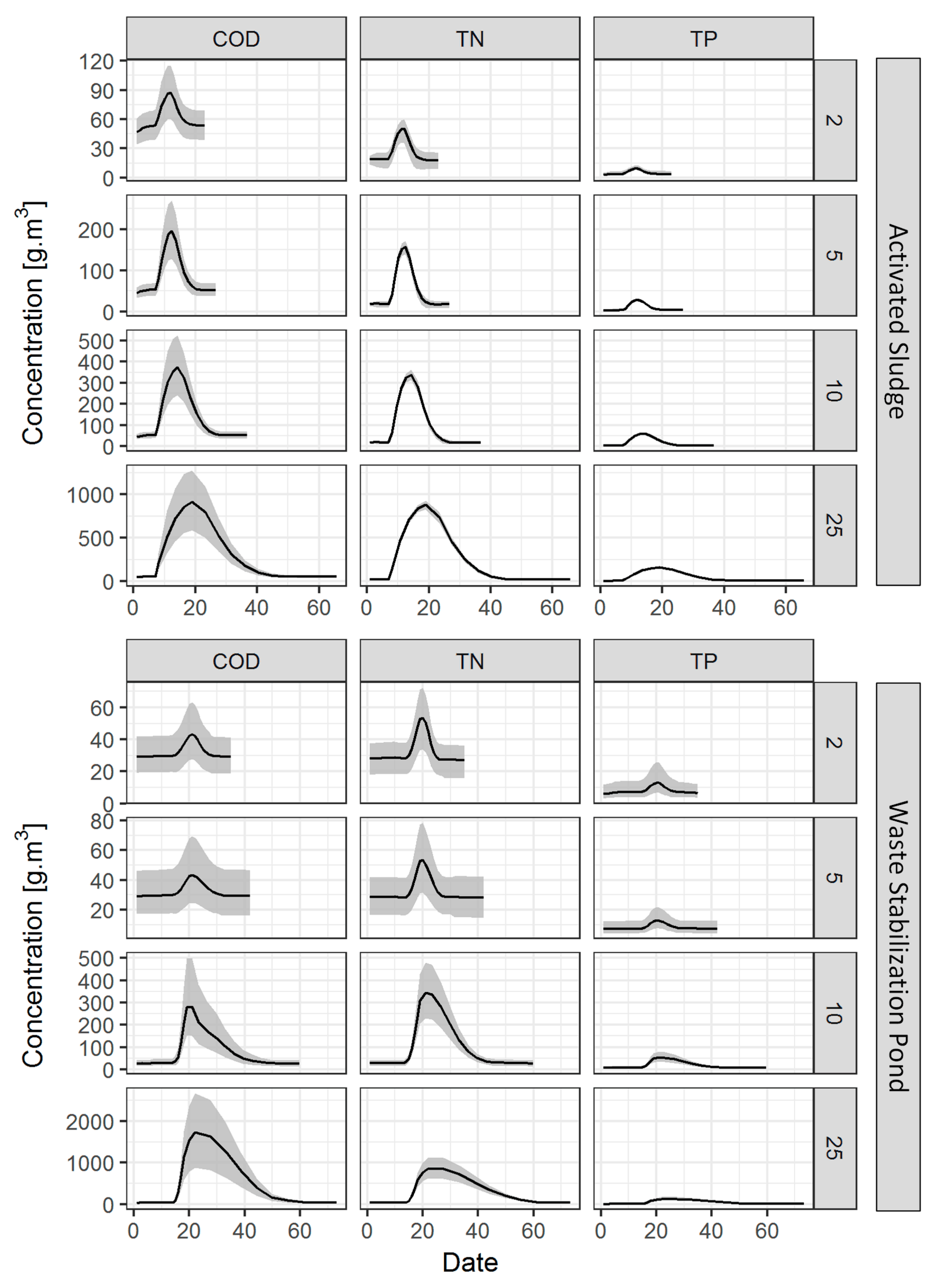
3.4. Scenario Analysis

The robustness of the two systems is analyzed via in silico experiments where different shock-load scenarios are simulated. These virtual experiments allow the provision of numerical responses of environmental systems to possible events in cooperation with a statistical technique for nonlinear error propagation. Figure 5 shows the performance and their uncertainty ranges of the AS and WSP systems in four scenarios varying from moderate to extreme influent concentrations. Generally speaking, the WSP can endure the peak load better than the AS system, except for the most extreme case of 25 times higher strength of wastewater. It is interesting that the natural system can produce comparable results of relatively low effluent concentrations when the wastewater strength increases from double to five times higher while the effluent quality of the AS system reduces by two times. This result highlights the robustness of WSPs in treating not only municipal wastewater with high strength, but also industrial wastewater with composition under 1500 mg COD·L⁻¹. However, when the wastewater strength increases higher, their durability is reduced. From the wastewater containing around 2700 mg COD·L⁻¹, WSPs show relatively similar removal efficiencies to AS systems. Especially at the last extreme scenario, their organic removal efficiency during the peak load is only half of that of the conventional biological treatment system. This deterioration reveals that with an extreme organic load of more than 7000 mg COD·L⁻¹, the conventional design of WSPs appears to be ineffective with very long recovery periods of up to 50 days. It is also noteworthy that the higher degree of complexity in the pond model compared to the AS model causes its broader uncertainty range, illustrating the intrinsic property of large model predictions. In fact, this overparameterization is also reflected in the calibrated value of model parameters, with few deviations compared to initial values as a result of the significantly lower number of available data for parameter estimation compared to the model complexity.

4. Conclusions

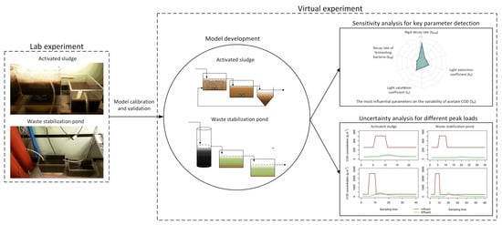
• We performed in silico experiments of four different shock-load scenarios in two sophisticated mechanistic models representing the two systems, i.e., AS and WSP. A systematic procedure of quality assurance for these virtual experiments was implemented to assess their uncertainty outputs, including sensitivity and uncertainty analysis with non-linear error propagation, and, more importantly, model calibration with a 210-day real experiment with 31 days of an increased load scenario. The simulation outputs highlight that the WSP can generally endure the increased load better than AS system, except with extremely high strength wastewater (over 7000 mg COD·L⁻¹), where a specific design focusing on the primary anaerobic pond is needed. From this result, the robustness of WSPs is proved suitable in treating not only municipal wastewater with high strength, but also industrial wastewater, such as poultry wastewater and paperboard wastewater. For further research, different characterizations of these types of wastewater could be applied in the two models to simulate their performance, and from that a concrete conclusion of preferential choice can be withdrawn. Besides removal performance, other factors related to plant footprint, operational and maintenance costs, energy efficiency, and greenhouse emissions should also be considered in this pre-selection process.
• The practical sensitivity analysis casts light on the most influential parameters on the performance of the conventional AS and pond systems. Particularly, as the AS system’s behavior is strongly dependent on the variability of oxygen, parameters related to autotrophic bacteria, the main oxygen consumer, initiate the most variability of particulate organic matter. PAOs emerges to be a main user of phosphorus whereas nitrogen removal is largely driven by nitrification and denitrification in the AS system. In contrast, the nutrient removal in the pond system is mostly done by algal assimilation while the absence of heterotrophs-related parameters indicates the insignificant role of the denitrification process. Also noteworthy is that the five top parameters in the importance-ranking list are all related to photosynthetic activity, which displays its crucial role in the pond performance.
• Model calibration displays a significant improvement in the prediction performance of the AS model, but not the WSP model. This contradictory result can be explained by the overparameterization of the large mechanistic model representing the natural system with numerous parameters and inputs, leading to a high requirement of both the quality and quantity of available data for proper calibration.
• The systematic model-based analysis proved to be a suitable mean for assessing the maximum load of wastewater treatment systems, thus avoiding environmental problems and high economic costs for cleaning surface waters after severe overload events. Moreover, these virtual experiments can be also a handy tool to find a proper solution for system overload, which is currently one of the main challenges of pond treatment technology.

References

- Verstraete, W.; Vlaeminck, S.E. Zerowastewater: Short-cycling of wastewater resources for sustainable cities of the future. Int. J. Sustain. Dev. World 2011, 18, 253–264. [Google Scholar] [CrossRef]
- United States Environmental Protection Agency. Principles of Design and Operations of Wastewater Treatment Pond Systems for Plant Operators, Engineers, and Managers; United States Environmental Protection Agency, Office of Research and Development: Washington, DC, USA, 2011.
- Ho, L.; Van Echelpoel, W.; Charalambous, P.; Gordillo, A.; Thas, O.; Goethals, P. Statistically-based comparison of the removal efficiencies and resilience capacities between conventional and natural wastewater treatment systems: A peak load scenario. Water 2018, 10, 328. [Google Scholar] [CrossRef]
- Ayyub, B.M. Systems resilience for multihazard environments: Definition, metrics, and valuation for decision making. Risk Anal. 2014, 34, 340–355. [Google Scholar] [CrossRef] [PubMed]
- Schoen, M.; Hawkins, T.; Xue, X.; Ma, C.; Garland, J.; Ashbolt, N.J. Technologic resilience assessment of coastal community water and wastewater service options. Sustain. Water Qual. Ecol. 2015, 6, 75–87. [Google Scholar] [CrossRef]
- Qureshi, N.; Shah, J. Aging infrastructure and decreasing demand: A dilemma for water utilities. J. Am. Water Works Assoc. 2014, 106, 51–61. [Google Scholar] [CrossRef]
- Bettini, Y.; Brown, R.; de Haan, F.J. Water scarcity and institutional change: Lessons in adaptive governance from the drought experience of Perth, Western Australia. Water Sci. Technol. 2013, 67, 2160–2168. [Google Scholar] [CrossRef] [PubMed]
- Omlin, M.; Reichert, P. A comparison of techniques for the estimation of model prediction uncertainty. Ecol. Model. 1999, 115, 45–59. [Google Scholar] [CrossRef]
- Reichert, P.; Vanrolleghem, P. Identifiability and uncertainty analysis of the river water quality model no. 1 (rwqm1). Water Sci. Technol. 2001, 43, 329–338. [Google Scholar] [CrossRef] [PubMed]
- Claeys, F.; Chtepen, M.; Benedetti, L.; Dhoedt, B.; Vanrolleghem, P.A. Distributed virtual experiments in water quality management. Water Sci. Technol. 2006, 53, 297–305. [Google Scholar] [CrossRef] [PubMed]
- Claeys, F. A Generic Software Framework for Modelling and Virtual Experimentation with Complex Environmental Systems. Ph.D. Thesis, Ghent University, Ghent, Belgium, 2008. [Google Scholar]
- Refsgaard, J.C.; Henriksen, H.J.; Harrar, W.G.; Scholten, H.; Kassahun, A. Quality assurance in model based water management—Review of existing practice and outline of new approaches. Environ. Model. Softw. 2005, 20, 1201–1215. [Google Scholar] [CrossRef]
- Todo, K.; Sato, K. Directive 2000/60/ec of the european parliament and of the council of 23 october 2000 establishing a framework for community action in the field of water policy. Environ. Res. Q. 2002, 66–106. [Google Scholar]
- Reichert, P. A standard interface between simulation programs and systems analysis software. Water Sci. Technol. 2006, 53, 267–275. [Google Scholar] [CrossRef] [PubMed]
- Refsgaard, J.C.; van der Sluijs, J.P.; Hojberg, A.L.; Vanrolleghem, P.A. Uncertainty in the environmental modelling process—A framework and guidance. Environ. Model. Softw. 2007, 22, 1543–1556. [Google Scholar] [CrossRef]
- Saltelli, A. Sensitivity analysis for importance assessment. Risk Anal. 2002, 22, 579–590. [Google Scholar] [CrossRef] [PubMed]
- OECD. Test No. 303: Simulation Test—Aerobic Sewage Treatment—A: Activated Sludge Units; B: Biofilms; OECD Publishing: Paris, France, 2001. [Google Scholar]
- Reichert, P. Aquasim—A tool for simulation and data analysis of aquatic systems. Water Sci. Technol. 1994, 30, 21–30. [Google Scholar] [CrossRef]
- Ho, L.; Pham, D.; Van Echelpoel, W.; Muchene, L.; Shkedy, Z.; Alvarado, A.; Espinoza-Palacios, J.; Arevalo-Durazno, M.; Thas, O.; Goethals, P. A closer look on spatiotemporal variations of dissolved oxygen in waste stabilization ponds using mixed models. Water 2018, 10, 201. [Google Scholar] [CrossRef]
- Ho, L.T.; Pham, D.T.; Van Echelpoel, W.; Alvarado, A.; Espinoza-Palacios, J.E.; Arevalo-Durazno, M.B.; Goethals, P.L.M. Exploring the influence of meteorological conditions on the performance of a waste stabilization pond at high altitude with structural equation modeling. Water Sci. Technol. 2018, 78, 37–48. [Google Scholar] [CrossRef] [PubMed]
- Langergraber, G.; Rousseau, D.P.L.; Garcia, J.; Mena, J. Cwm1: A general model to describe biokinetic processes in subsurface flow constructed wetlands. Water Sci. Technol. 2009, 59, 1687–1697. [Google Scholar] [CrossRef] [PubMed]
- Sah, L.; Rousseau, D.P.L.; Hooijmans, C.M.; Lens, P.N.L. 3d model for a secondary facultative pond. Ecol. Model. 2011, 222, 1592–1603. [Google Scholar] [CrossRef]
- Brun, R.; Reichert, P.; Kunsch, H.R. Practical identifiability analysis of large environmental simulation models. Water Resour. Res. 2001, 37, 1015–1030. [Google Scholar] [CrossRef]
- Omlin, M.; Brun, R.; Reichert, P. Biogeochemical model of Lake Zurich: Sensitivity, identifiability and uncertainty analysis. Ecol. Model. 2001, 141, 105–123. [Google Scholar] [CrossRef]
- Mieleitner, J.; Reichert, P. Modelling functional groups of phytoplankton in three lakes of different trophic state. Ecol. Model. 2008, 211, 279–291. [Google Scholar] [CrossRef]
- Brun, R.; Kuhni, M.; Siegrist, H.; Gujer, W.; Reichert, P. Practical identifiability of asm2d parameters—Systematic selection and tuning of parameter subsets. Water Res. 2002, 36, 4113–4127. [Google Scholar] [CrossRef]
- Weijers, S.R.; Vanrolleghem, P.A. A procedure for selecting best identifiable parameters in calibrating activated sludge model no.1 to full-scale plant data. Water Sci. Technol. 1997, 36, 69–79. [Google Scholar] [CrossRef]
- Dochain, D.; Vanrolleghem, P.A. Dynamical Modelling & Estimation in Wastewater Treatment Processes; IWA Publishing: London, UK, 2001. [Google Scholar]
- Reichert, P. Uncsim a Computer Programme for Statistical Inference and Sensitivity, Identifiability, and Uncertainty Analysis. 2005. Available online: https://pdfs.semanticscholar.org/126b/2a369fdfdc3f02f40a7d310db077595400f9.pdf (accessed on 28 May 2017).
- Joseph, A. Scenarios as Tools for International Environmental Assessment; European Environment Agency: Copenhagen, Denmark, 2001. [Google Scholar]
- Robert, C.; Casella, G. Monte Carlo Statistical Methods, 2nd ed.; Springer: New York, NY, USA, 2004. [Google Scholar]
- Henze, M.; Guijer, W.; Mino, T.; van Loosdrecht, M. Activated Sludge Models asm1, asm2, asm2d and asm3; IWA Publishing: London, UK, 2000. [Google Scholar]
- Ferrero, C.S.; Chai, Q.; Diez, M.D.; Amrani, S.H.; Lie, B. Systematic analysis of parameter identifiability for improved fitting of a biological wastewater model to experimental data. Model. Identif. Control 2006, 27, 219–238. [Google Scholar] [CrossRef]
- Liau, K.F.; Shoji, T.; Ong, Y.H.; Chua, A.S.M.; Yeoh, H.K.; Ho, P.Y. Kinetic and stoichiometric characterization for efficient enhanced biological phosphorus removal (ebpr) process at high temperatures. Bioproc. Biosyst. Eng. 2015, 38, 729–737. [Google Scholar] [CrossRef] [PubMed]
- Henze, M.; van Loosdrecht, M.; Ekama, G.A.; Brdjanovic, D. Biological Wastewater Treatment: Priniciples, Modelling and Design; IWA Publishing: London, UK, 2008. [Google Scholar]
- Ho, L.T.; Van Echelpoel, W.; Goethals, P.L.M. Design of waste stabilization pond systems: A review. Water Res. 2017, 123, 236–248. [Google Scholar] [CrossRef] [PubMed]
- Yagci, N.; Dulekgurgen, E.; Artan, N.; Orhon, D. Experimental evaluation and model assessment of coexistence of paos and gaos. J. Environ. Sci. Health A 2011, 46, 968–979. [Google Scholar] [CrossRef] [PubMed]
- Freni, G.; Mannina, G.; Viviani, G. Identifiability analysis for receiving water body quality modelling. Environ. Model. Softw. 2009, 24, 54–62. [Google Scholar] [CrossRef]
- Shilton, A. Pond Treatment Technology; IWA Publishing: London, UK, 2005. [Google Scholar]