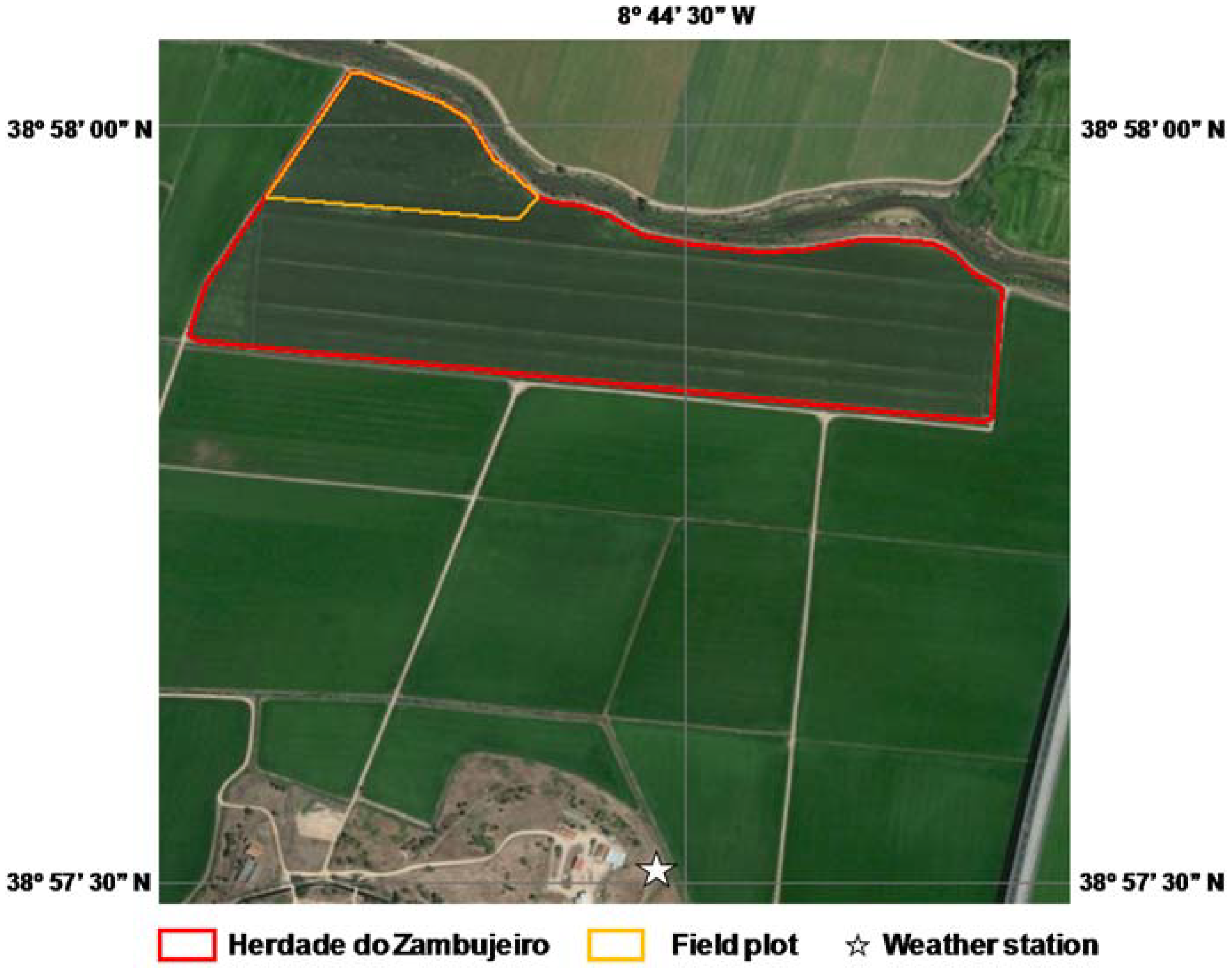
2.1. Field Site Description and Data
Field data used in this study was collected at Herdade do Zambujeiro (22 ha), Benavente, southern Portugal (38°58′0.97′′ N, 8°44′46.63′′ W, 6 m a.s.l.) (
Figure 1). The climate in the region is semi-arid to dry sub-humid, with hot dry summers and mild winters with irregular rainfall. The mean annual temperature is 16.8 °C, with the mean daily temperatures at the coolest (January) and warmest (August) months reaching 11.4 and 22.7 °C, respectively. The mean annual precipitation is 668 mm, mostly occurring between October and May. The soil was a Haplic Fluvisol [
34], with the main soil physical and chemical properties presented in
Table 1. The bottom layers exhibited higher dry bulk density and lower measured saturated hydraulic conductivity values than the topsoil layers [
3], evidencing some soil compaction due to tillage operations carried out throughout the years and the relatively high soil moisture that was constant along the seasons because of the shallow groundwater levels.
The MOHID-Land model was previously implemented in the area by Ramos et al. [
3]. These authors evaluated the model’s capacity in predicting soil water contents and fluxes and the evolution of different crop growth parameters, including the leaf area index (LAI), canopy height, aboveground dry biomass and yields during the 2014 and 2015 maize growing seasons. Details on the calibration/validation approach can be found in the cited reference. For that, the field was cropped with maize hybrid P1574 (FAO 600) with a density of approximately 89,000 plants ha
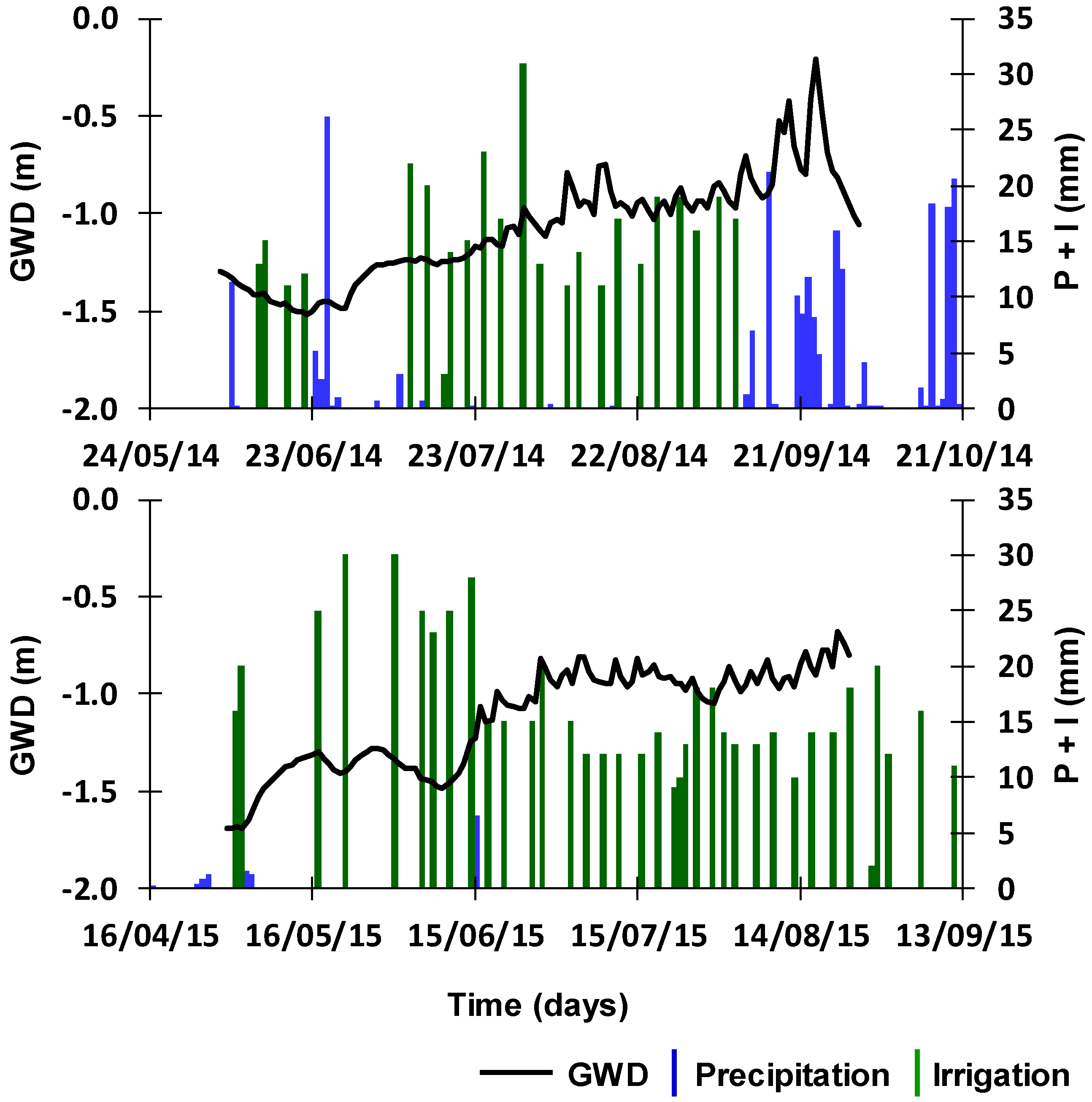
−1. Management practices, including fertilization and irrigation, were performed according to the standard practices in the region and were decided by the farmer. During 2014, maize was sown on May 24 and harvested on October 8; the net rainfall reached 163 mm, while the net irrigation amounted 365 mm (
Figure 2). During 2015, maize was sown on April 16 and harvested on September 20; the net rainfall reached only 12 mm, while the net irrigation summed 620 mm (
Figure 2). Irrigation was applied with the farmer’s stationary sprinkler system. Groundwater depth (GWD) varied between approximately 1.5 m depth at the beginning of the growing season to 1.0 m depth during irrigation, further reaching 0.3 m depth during September 2014 after successive rain events (
Figure 2). Crop stages were set as in
Table 2 based on field observations.
One SM1 capacitance probe (Adcon Telemetry, Klosterneuburg, Austria) and one ECH2O-5 capacitance probe (Decagon Devices, Pullman, WA, USA) were installed at depths of 10, 30 and 50 cm to continuously measure soil water contents. One LEV1 level sensor (Adcon Telemetry, Klosterneuburg, Austria) was used to continuously monitor the groundwater level (
Figure 2). One RG1 (Adcon Telemetry, Klosterneuburg, Austria) and two QMR101 (Vaisala, Helsinki, Finland) rain gauges were used to measure the amount of water applied per irrigation event.
LAI, canopy height and the aboveground dry biomass were further monitored by harvesting 3 random plants in four locations distributed randomly throughout the field plot, every 15 days, between May and September, during the 2014 and 2015 maize growing seasons (
Table 3). The same crop parameters were measured at the end of each crop season, but by harvesting all plants in random areas of 1.5 m
2 (corresponding to approximately 12 plants). The length and width of crop leafs were measured in every harvested plant and then converted to LAI values as documented in Ramos et al. [
4]. The aboveground dry biomass was determined by oven drying maize stems, leaves and grain at 70 °C to a constant weight. Maize yield was obtained from the grain’s dry biomass measured at the end of each crop season.
2.2. Model Description
MOHID-Land is a distributed model capable of computing different physical and chemical processes in a three-dimensional domain using a finite-volume approach [
27]. Variably-saturated water flow is described using the Richards equation, while the van Genuchten–Mualem functional relationships [
35] are used for defining the unsaturated soil hydraulic properties, as follows:
where S
e is the effective saturation (L
3 L
−3), θ
r and θ
s denote the residual and saturated water contents (L
3 L
−3), respectively, K
s is the saturated hydraulic conductivity (L T
−1), α (L
−1) and η (-) are empirical shape parameters, m = 1 − 1/η and
is a pore connectivity/tortuosity parameter (-).
Crop evapotranspiration (ET
c) is determined from reference evapotranspiration (ET
0) values computed with the FAO Penman-Monteith method using the single crop coefficient (K
c) approach [
36]. ET
c is then partitioned into potential soil evaporation (E
p) and potential crop transpiration (T
p) as a function of LAI [
37]:
where λ is the extinction coefficient of radiation attenuation within the canopy (-).
Root water uptake is computed using the macroscopic approach introduced by Feddes et al. [
38], meaning that T
p is distributed over the root zone and may be diminished by the presence of depth-varying root zone stressors, namely water stress. Root water uptake reductions (i.e., actual transpiration, T
a) are then described using the piecewise linear model proposed by Feddes et al. [
38]. In this model, root water uptake is at the potential rate when the pressure head (h) is between h
2 and h
3, drops off linearly when h > h
2 or h < h
3 and becomes zero when h < h
4 or h > h
1 (subscripts 1 to 4 denote for different threshold pressure heads). E
p values are limited by a pressure head threshold value to obtain the actual soil evaporation rate (E
a) [
39].
MOHID-Land further includes a modified version of the EPIC model [
40,
41] for simulating crop growth. This model is based on the heat unit theory, which considers that all heat above the base temperature will accelerate crop growth and development:
where PHU is the total heat units required for plant maturity (°C), HU is the number of heat units accumulated on day i (°C), i = 1 corresponds to the sowing date (-), m is the number of days required for plant maturity (-), T
av is the mean daily temperature (°C) and T
base is the minimum temperature for plant growth (°C).
Crop growth is modelled by simulating light interception, conversion of intercepted light into biomass and LAI development. Total biomass is calculated from the solar radiation intercepted by the crop leaf area using the Beer’s law [
42]:
where ΔBio
act,i and ΔBio
i are the actual and potential increase in total plant biomass on day i (kg ha
−1), RUE is the radiation-use efficiency of the plant ((kg ha
−1) (MJ m
−2)
−1), PAR
i is the daily incident photosynthetically active radiation (MJ m
−2), λ is again the light extinction coefficient (-) and γ
i is the daily plant growth factor (0–1) which accounts for water and temperature stresses [
41].
Leaf area index is computed as a function of heat units, crop stress and the development stage [
41]. During early stages (initial and plant development stages), LAI increment on a given day is a function of the fraction of the plant’s maximum LAI (LAI
max) that needs to be reached during those stages (fr
LAImax) and crop stress.
where ΔLAI
act,i and ΔLAI
i are the actual and potential LAI increment added on day i (m
2 m
−2), respectively and fr
LAImax,i and fr
LAImax,i−1 are the fraction of the plant’s maximum LAI (LAI
max, m
2 m
−2) on day i and i − 1 (-), respectively. During the mid-season stage, LAI is assumed to be constant. During the late-season stage, LAI declines as a function of LAI
max, heat units and crop stress.
Root depth is also computed as a function of heat units [
41], while root biomass is assumed to decrease from 0.4 of the total biomass at emergence to 0.2 at maturity [
43]. Finally, yield is obtained from the product of the aboveground dry biomass and the actual harvest index [
41]. A more detailed description of the MOHID-Land model governing equations can be found in Trancoso et al. [
27] and Ramos et al. [
3].
2.3. Model Setup and Data Assimilation
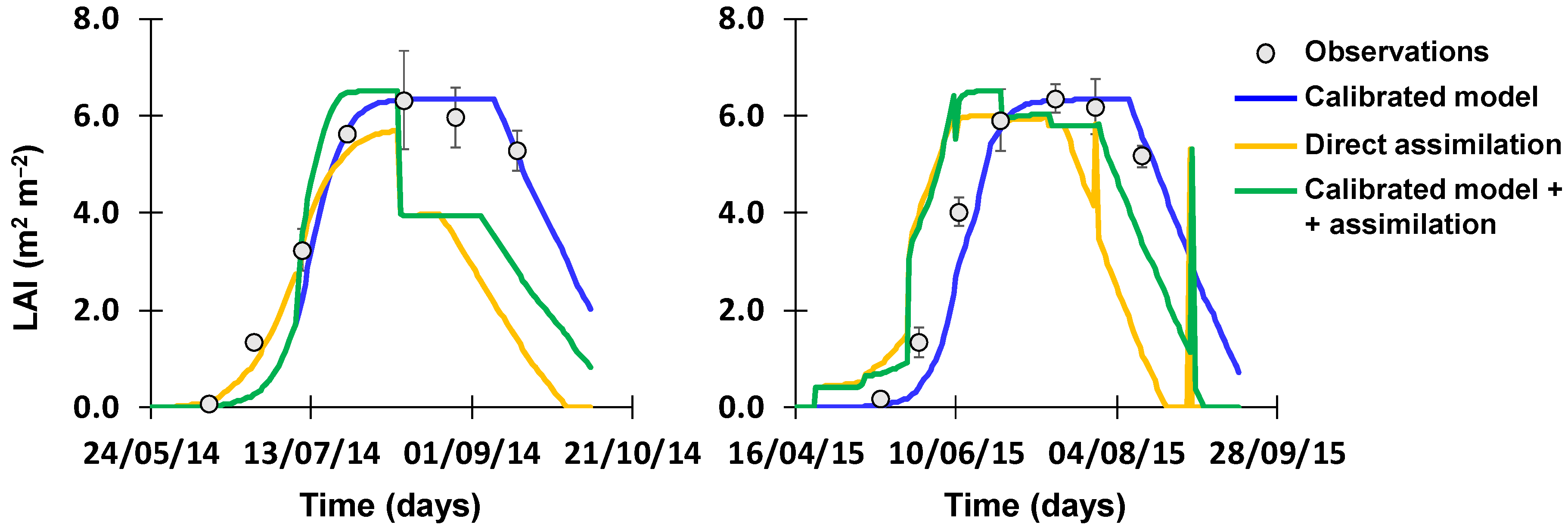
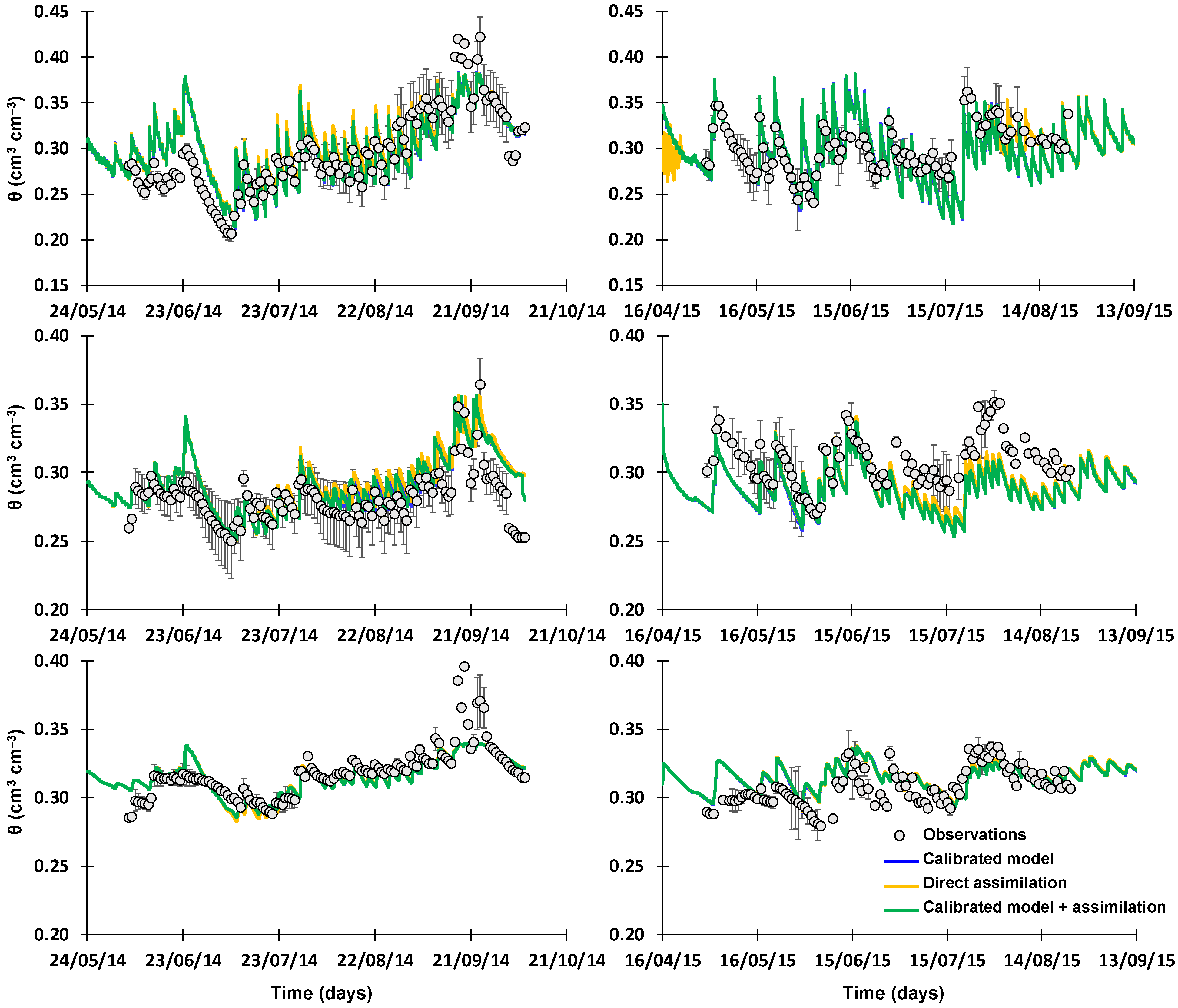
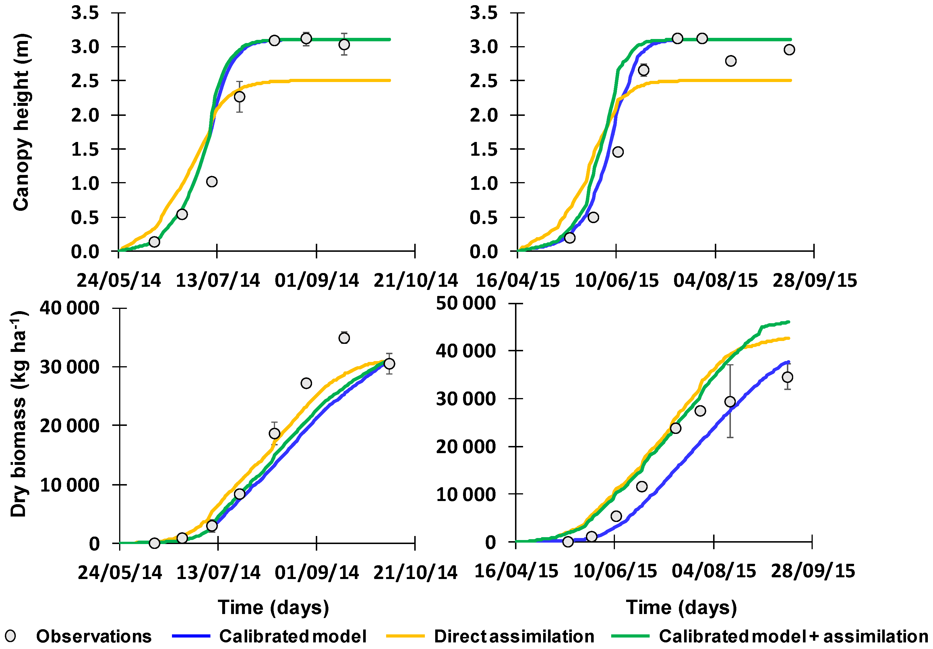
The assimilation of LAI data into MOHID-Land simulations has a direct influence on the water balance through the partition of ETc values into Tp (Equation (3)) and Ep (Equation (4)) and on the computation of the aboveground dry biomass (Equation (6)) Three distinct approaches were thus considered for better understanding the impact of LAI assimilation on model simulations:
A—The model was run as in Ramos et al. [
3], which simulations of soil water contents, LAI, h
c, aboveground dry biomass and yields served as baseline for this study (Calibrated model). These authors followed a traditional calibration/validation approach, where a trial-and-error procedure was carried out to adjust soil hydraulic (
Table 1) and crop parameters (
Table 4) until deviations between the measured 2014 dataset and simulated values were minimized. The calibrated parameters were then validated using the 2015 dataset, with model simulations being compared to measured data.
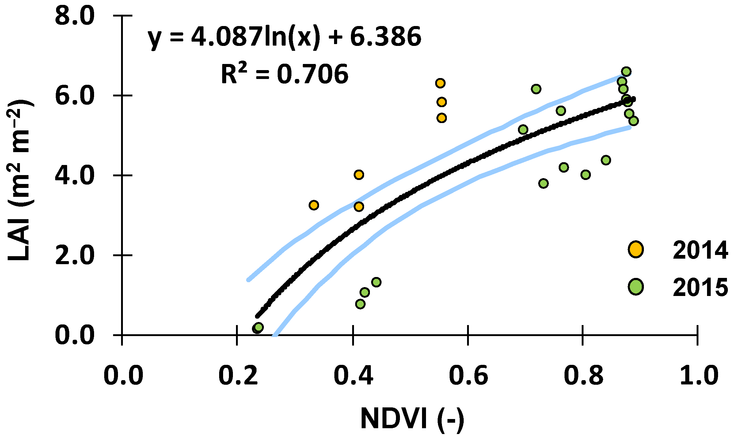
B—The model was run using LAI values extracted from satellite data as inputs (LAI assimilation). LAI values were derived from the normalized difference vegetation index (NDVI) using the relationship shown in
Figure 3. This relationship was found by comparing NDVI values computed from Landsat 8 satellite images (band 4 and 5) with LAI values measured in the study site, at multiple locations and over the 2014 and 2015 growing seasons. The calibrated soil hydraulic parameters were here also adopted (
Table 1). However, the default crop parameters from the MOHID-Land’s database (
Table 4) were considered instead so that model performance in the absence of a calibrated dataset could be assessed.
C—The model was again run using LAI values extracted from satellite data as inputs. However, Ramos et al. [
3] calibrated crop parameters (
Table 4) were here considered (Calibration + LAI assimilation), as well as the calibrated soil hydraulic parameters (
Table 1).
Landsat 8 images were first corrected to convert the TOA (Top of Atmosphere) planetary reflectance using reflectance rescaling coefficients provided in the Landsat 8 OLI metadata file and to correct the reflectance value with the sun angle. Two images were available from sowing to harvest during the 2014 growing season, while eight images were used during the 2015 growing season (
Table 5). These images were used to extract the NDVI values corresponding to the multiple locations where LAI field observations were carried out, in a total of 26 measurements (
Figure 3). LAI and NDVI values ranged from 0.41–5.85 and 0.23–0.88, respectively, in line with Pôças et al. [
44].
Data assimilation in MOHID-Land was carried out using the forcing method [
12]. The approach is relatively straightforward, with the model simply replacing the predicted value by a new input when an image becomes available, updating then fr
LAImax to account for what still needs to be reached during a specific crop stage and more interestingly, the water balance and the aboveground dry biomass estimates. From that date on and until another image becomes available model simulations follow the parameterization given in
Table 4.
Table 5 lists the assimilated LAI values and dates.
In all simulations (Approach A–C), the soil profile was specified with 2 m depth, divided into four soil layers according to observations (
Table 1). The soil domain was represented using an Arakawa C-grid type [
45], defined by one vertical column (one-dimensional domain) discretized into 100 grid cells with 1 m wide, 1 m long and 0.02 m thickness each (i.e., 1 × 1 × 0.02 m
3). The simulation periods covered from sowing to harvest. The upper boundary condition was determined by the actual evaporation and transpiration rates and the irrigation and precipitation fluxes (
Figure 2). Weather data used in this study was taken from a meteorological station located 950 m from the study site (38°57′30.25′′ N, 8°44′31.70′′ W, 7 m a.s.l.;
Figure 1) and included the average temperature (°C), wind speed (m s
−1), relative humidity (%), global solar radiation (W m
−2) and precipitation (mm). ET
c values were computed from hourly ET
0 values and K
c values of 0.30, 1.20 and0.35 for the initial, mid-season and late season crop stages, respectively [
31]. The K
c value for the initial crop stage was then adjusted for the frequency of the wetting events (precipitation and irrigation) and average infiltration depths, while the K
c values for mid-season and late season crop stages were adjusted for local climate conditions taking into consideration canopy height, wind speed and minimum relative humidity averages for the periods under consideration [
36]. The following parameters of the Feddes et al. [
38] model were used to compute T
p reductions due to water stress: h
1 = −15, h
2 = −30, h
3 = −325 to −600, h
4 = −8000 cm [
46]. The bottom boundary condition was specified using the observed GWD (
Figure 2). The initial soil water content conditions were set to field capacity.
2.4. Statistical and Uncertainty Analysis
Model calibration and validation was performed by comparing field measured values of soil water contents, LAI, h
c and aboveground dry biomass with the MOHID-Land simulations (Approaches A–C) using various quantitative measures of the uncertainty, such as, the coefficient of determination (R
2), the root mean square error (RMSE), the ratio of the RMSE to the standard deviation of observed data (NRMSE), the percent bias (PBIAS) and the model efficiency (EF). R
2 values close to 1 indicate that the model explains well the variance of observations. RMSE, NRMSE and PBIAS values close to zero indicate small errors of estimate and good model predictions [
47,
48,
49]. Positive or negative PBIAS values refer to the occurrence of under- or over-estimation bias, respectively. Nash and Sutcliff [
50] modelling efficiency EF values close to 1 indicate that the residuals variance is much smaller than the observed data variance, hence the model predictions are good; contrarily, when EF is very close to 0 or negative there is no gain in using the model.
Data assimilation is much dependent on the empirical relationship (
Figure 3) established to derive LAI values from the NDVI measurements [
14,
18]. As such, the uncertainty related to that conversion was quantified on final model estimates of T
a, E
a and aboveground dry biomass using a Monte Carlo method. This evaluation was performed on modeling Approach C (Calibration + LAI assimilation) as the objective here was to assess if remote sensing data assimilation could further correct for simulation errors that result from model parameter uncertainty. The 2015 dataset was also considered as more satellite images were available during this season. A randomly population of 10,000 LAI values was first created for each available image date following a normal distribution with mean equal to the estimated parameter given by the LAI-NDVI regression equation and range defined by the 95% confidence intervals (
Figure 3,
Table 5). The model was then run following Approach C settings until reaching the dates of each of the eight available images (8 × 1 simulation). Afterwards, the 10,000 LAI randomly generated values were assimilated by the model, which then proceeded with simulations until the end season following Approach C settings again (8 × 10,000 simulations). In the end, the uncertainty of final model estimates of T
a, E
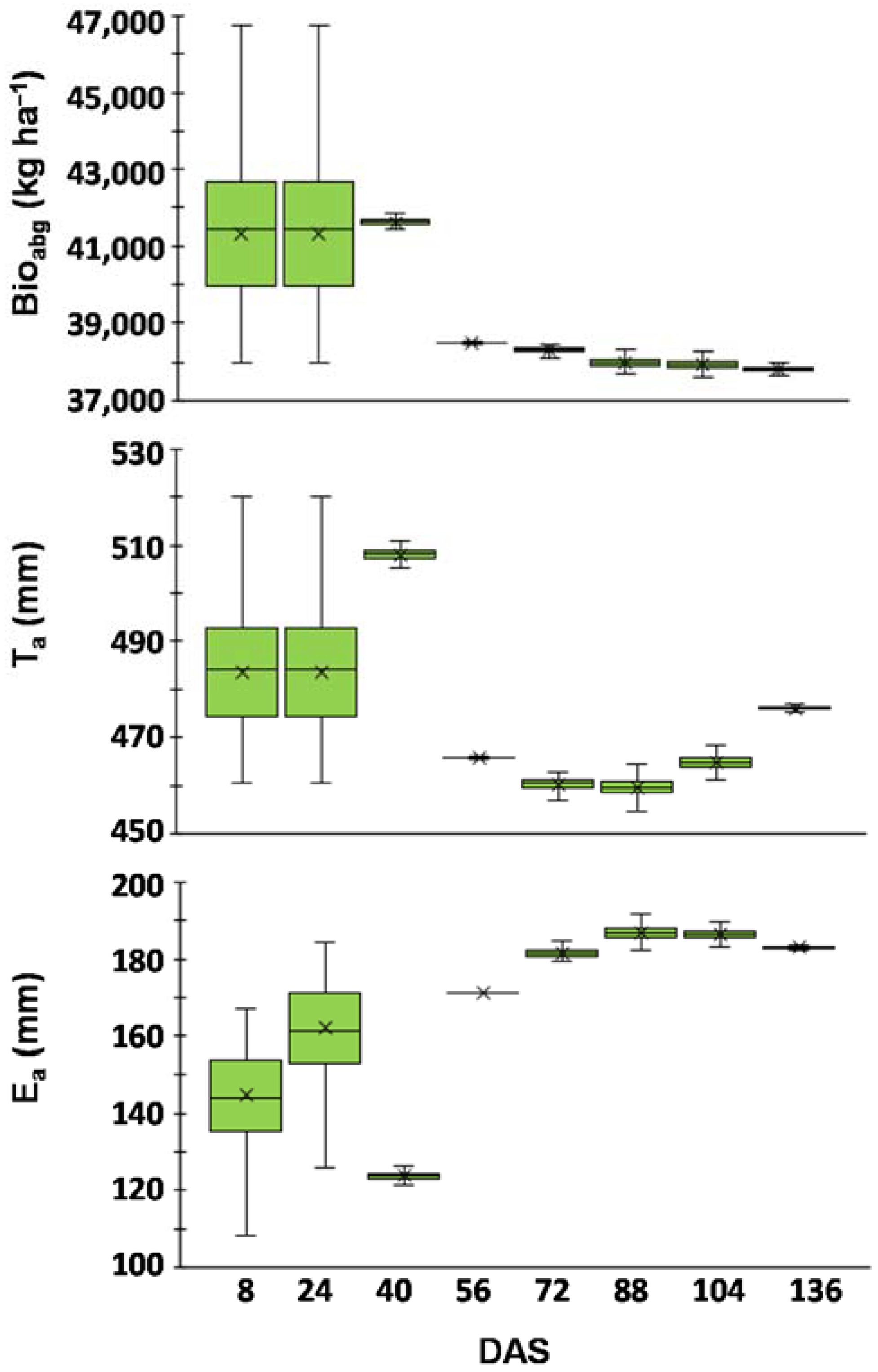
a and aboveground dry biomass were assessed for each assimilation date (8 dates) from 10,000 simulations (80,000 simulations in total). The Monte Carlo simulations were performed with a Python script.


