Rainfall-Induced Landslide Susceptibility Using a Rainfall–Runoff Model and Logistic Regression

Abstract

Conventional landslide susceptibility analysis adopted rainfall depth or maximum rainfall intensity as the hydrological factor. However, using these factors cannot delineate temporal variations of landslide in a rainfall event. In the hydrological cycle, runoff quantity reflects rainfall characteristics and surface feature variations. In this study, a rainfall–runoff model was adopted to simulate the runoff produced by rainfall in various periods of a typhoon event. To simplify the number of factors in landslide susceptibility analysis, the runoff depth was used to replace rainfall factors and some topographical factors. The proposed model adopted the upstream area of the Alishan River in southern Taiwan as the study area. The landslide susceptibility analysis of the study area was conducted by using a logistic regression model. The results indicated that the overall accuracy of predicted events exceeded 80%, and the area under the receiver operating characteristic curve (AUC) closed to 0.8. The results revealed that the proposed landslide susceptibility simulation performed favorably in the study area. The proposed model could predict the evolution of landslide susceptibility in various periods of a typhoon and serve as a new reference for landslide hazard prevention.

1. Introduction

Landslide susceptibility analysis can be divided into qualitative and quantitative analyses [1]. Qualitative analysis methods are subjective recognition methods whose analysis results vary according to the practical experiences and comprehensive analysis capabilities of the judging person. These methods are usually applied to analyze landslide susceptibility when comprehensive data are lacking. However, because of the subjective nature of qualitative analysis, it is difficult to apply conventional judgements of reliability and validity, and the qualitative analysis has been gradually replaced by the quantified analysis. Qualitative analysis methods include statistical analyses, artificial neural networks, and deterministic seismic hazard analysis. These methods involve collecting a sufficient amount of data on historical landslide events, quantifying their variables, and establishing a model to predict landslide occurrence. Recently, statistical methods have become the main form of landslide susceptibility analysis [2]. In statistical analysis methods, logistic regression adopts influencing factors of landslides as independent variables and landslide occurrence (or nonoccurrence) as the dependent variable to obtain a logistic regression equation with which to predict the relationship between the dependent and independent variables. Independent variables can include continuous and categorical variables, and thus have relatively few application restrictions. Hence, numerous scholars have adopted logistic regression in landslide susceptibility analysis [1,3,4,5,6,7,8,9,10,11,12].

More than 60 factors have been discussed in relation to landslide susceptibility analysis [13]. These factors can be grouped into static environmental factors and dynamic external triggering factors. Environmental factors indicate the natural environment of the slope and can be categorized into topographical, geological, and location factors. Topographical factors are used to represent the surface features of the research site, including elevation, aspect, and slope gradient. Slope is the most frequently adopted factor in landslide studies. The slope gradient influences the landslide susceptibility of a slope [5]; in particular, the correlation between the slope and the landslide occurrence is substantially increased when the slope is a uniform homogenous isotropic one. The field investigations of shallow landslides in mountainous areas of Taiwan indicated that slope gradient is a key factor influencing landslides [14]. Shallow landslides in mountainous areas of Taiwan mostly occurred on slopes with a gradient lower than 50°, in particular those with a gradient of 30°–40°. Geological factors reflect geological structure of a slope. The lithology in geological factors is a critical factor of landslide occurrence [1]. The slopes with fragile lithological conditions are highly susceptible to landslides. Location factors refer to factors that exist in the environment that can influence slope stability, such as water systems, roads, and faults. Triggering factors play a critical role in introducing external forces for landslides such as rainfall, snow melting, volcano eruptions, and earthquakes. Taiwan is located in the northwestern Pacific Ocean, where approximately 25.2 typhoons occur every year, ranking first in terms of typhoon formulation frequency in the world. In addition, Taiwan is located in a critical area for typhoon turning resulting in approximately 3.6 typhoons hitting Taiwan each year [15]. Therefore, heavy rainfall caused by typhoons is the main triggering factor of landslides in Taiwan.

Rainfall exerts a negative influence on slope stability primarily through rain that permeates into the ground. Permeated rain lowers the effective stress and shear mass of the soil, leading to slope landslides [16]. However, the effect of permeated rain on slope stability is difficult to quantify. Only by conducting mechanical analysis on permeating behaviors in relation to the slope safety coefficient can the influences of rainfall on slope stability be revealed. Therefore, quantified analysis for the influence of rainfall on landslide susceptibility has focused on specific rainfall factors. Factors frequently used to indicate rainfall characteristics include rainfall intensity, rainfall duration, daily rainfall, single-event rainfall depth, and rainfall kinetic energy. The rainfall factors used in landslide susceptibility analysis were discussed in-depth in [17]. Efforts have also been made to improve the predictions using various rainfall factors [18,19]. However, by using a single factor it is difficult to determine whether that factor is qualified to represent the characteristics of the entire rainfall event. Rainfall characteristics vary by weather conditions and topographical characteristics, and this causes considerable temporal and spatial differences in a rainfall event.

The hydrological cycle indicates that after a rainfall event, surface runoff occurs, and its amount is dependent on the water loss in the catchment area and the temporal and spatial variations in rainfall distribution. Surface runoff is a key influencing factor of the actual infiltration of surface runoff in the catchment area. Infiltration tends to saturate soil, thereby enhancing the probability of slope landslide occurrence. In the present study, a rainfall-runoff model was adopted to simulate the runoff produced by rainfall in various periods. Instead of rainfall depth or rainfall intensity, the proposed model adopted runoff depth—because of its relevance in terms of physics—as the triggering factor of landslide susceptibility. Runoff was also considered to serve as a replacement for some topographical factors in landslide susceptibility analysis, thereby reducing the number of factors. A flowchart of this study is shown in Figure 1. In addition, because of recent rapid developments in computer technology, geographic information systems (GIS) are a powerful tool for landslide susceptibility analysis. This study conducted rainfall runoff and landslide susceptibility analyses using a GIS, which enabled effective data construction, analysis, and display. A GIS can integrate substantial topographical and hydrological data to achieve fast recognition of the changes of landslide situations during a rainfall event. This study proposed a methodological framework for predicting the landslide susceptibility of various locations at various time. The resultant new information can serve as a reference for governance planning and disaster relief. In the future, this method could be combined with rainfall prediction data to construct a landslide hazard early warning system.

2. Materials and Methods

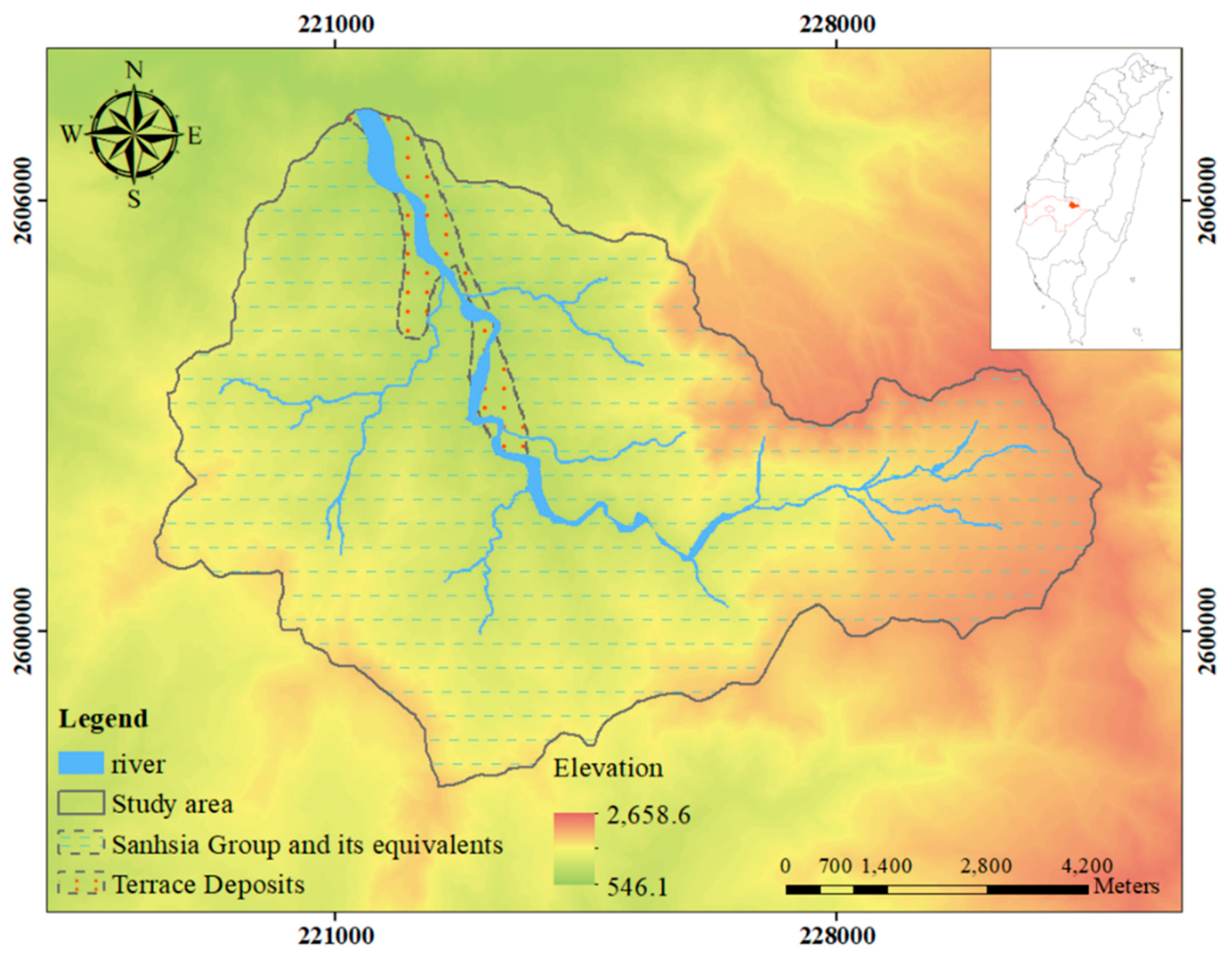
2.1. Study Area

The Alishan River is located in southern Taiwan. The elevation of the watershed ranges from 545 m to 2660 m and the aspect in most areas is northwestern (19.1%) or northern (15.9%). The watershed features steep terrains; approximately 55.9% of the area has a slope gradient greater than 55%. Regarding geological distribution, more than 95% of the catchment area comprises late-Miocene Sanhsia Group Kueichulin formation, whereas only a small part consists of Pleistocene terrace deposits. The Alishan River is located in the subtropical climate zone. In summer, thunderstorms and typhoons bring torrential rain to this area. The area is on the windward side of the torrential rain. Hence, this area is cloudy and humid. Rainfall data from 2000–2017 collected at the nearby Fenqihu Rainfall Station revealed that the average annual rainfall in this area is 4202 mm, which is substantially higher than that in Taiwan (2500 mm). Rainfall in this area mostly occurs in summer, particularly during the typhoon and torrential rain season of July to September, followed by the monsoon season of May and June. Accumulated rainfall in the flood season, namely between May and November, accounts for approximately 89.8% of the annual rainfall depth of this area. Because heavy rain often leads to landslides in the area of the Alishan River, it severely threatens the life and property of local residents. Therefore, the upstream area of the Alishan River was selected as the study area (Figure 2). It covers an area of about 67 km². Because landslide occurrence is highly correlated with geological features, landslides primarily occur under specific geological conditions. The geological distribution indicates that the spatial variation of the geological conditions within the study area is negligible. Hence, conducting landslide susceptibility analysis in this area can prevent geological factors from directly influencing the results. The proposed rainfall-runoff model was adopted to predict landslides caused by typhoon events in the study area and evaluate the model performance in landslide susceptibility analysis.

2.2. Basic Data Collection

The cartographic resources used in this study were a geological map with a scale of 1:250,000, a land use map, a 5 m × 5 m high-precision digital elevation model, a road map, and a drainage map. The spatial distribution of the factors required for subsequent analysis was extracted using the GIS. Regarding landslide recognition in the research site, satellite images before and after typhoon events were compared. Then, the new and expanded landslides were mapped. The analysis showed that Typhoon Talim in August 2005 and Typhoon Jangmi in October 2008 both caused substantial landslides in the Alishan area. These two typhoons resulted in 139.65 and 92.23 hectares of landslide in the study area, respectively, which corresponded to 2.98% and 1.38% of the total area. Thus, the rainfall-runoff model was employed to analyze the variations of runoff distributions in the study area during these two typhoons. Subsequently, landslide susceptibility analysis was performed and incorporated runoff quantity and other factors.

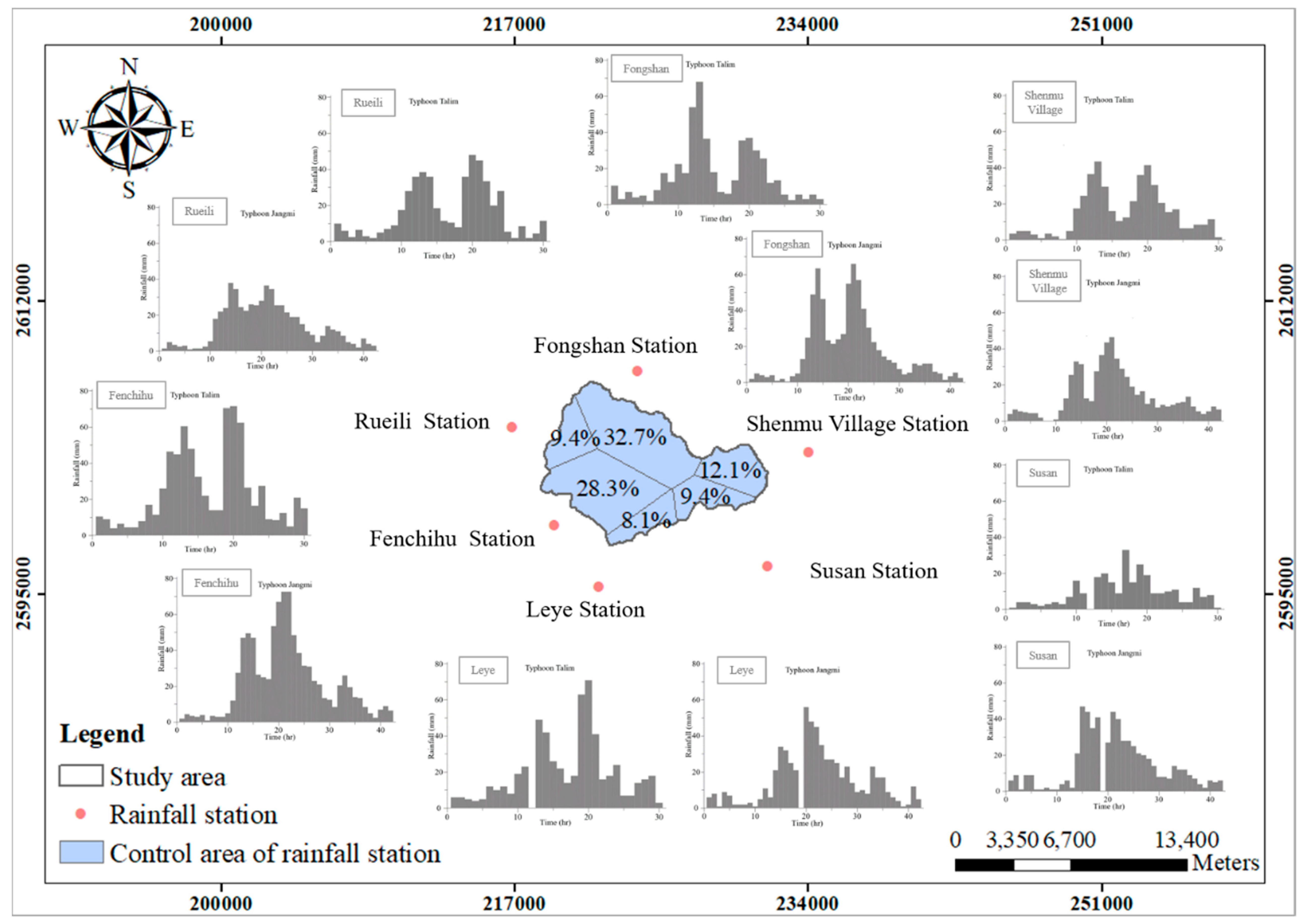
2.3. Rainfall Distribution Estimation

For effective analysis of runoff variation in the study area during the typhoon rainfall periods, temporal and spatial variations in rainfall characteristics were considered when conducting the rainfall-runoff analysis. Hourly rainfall data from six nearby rainfall stations, namely Shenmu Village, Fenqihu, Ruili, Fengshan, Shuishan, and Leye Rainfall Stations, were adopted in this study. Spatial distributions of rainfall data were estimated based on these data through the Thiessen polygon method [20]. Figure 3 displays the rainfall station distribution and control area of each rainfall station in the study area. Each control area contains a rainfall station. Rainfall within a control area was assumed to be represented by the rainfall data of the rainfall station.

Table 1. Rainfall Characteristics of six rainfall stations during Typhoon Talim and Typhoon Jangmi.

Rainfall Station	Typhoon Talim			Typhoon Jangmi
	Rainfall Duration: 30 h			Rainfall Duration: 42 h
	Rainfall Depth (mm)	Maximum Rainfall Intensity (mm/h)	Averaged Rainfall Intensity (mm/h)	Rainfall Depth (mm)	Maximum Rainfall Intensity (mm/h)	Averaged Rainfall Intensity (mm/h)
Shenmu Village	444.5	43.5	14.8	584.0	46.5	13.9
Fenqihu	730.0	71.5	24.3	919.5	75.0	21.9
Rueili	500.0	48.0	16.7	591.0	38.0	14.1
Fengshan	491.0	68.0	16.4	733.5	66.0	17.5
Shuishan	285.0	33.0	9.5	605.0	47.0	14.4
Leye	588.0	80.0	19.6	636.0	56.0	15.1

lists the statistics for rainfall data recorded at six rainfall stations during Typhoon Talim and Typhoon Jangmi. The rainfall durations of these two typhoons were 30 and 42 h, respectively. Rainfall due to both typhoons was concentrated around Fenqihu Rainfall Station. Typhoon Jangmi exhibited a greater rainfall depth and higher maximum rainfall. During Typhoon Talim, the rainfall depth and maximum rainfall at Fenqihu Rainfall Station were 730.0 and 71.5 mm, respectively. The corresponding characteristics during Typhoon Jangmi were 919.5 and 75.0 mm, respectively.

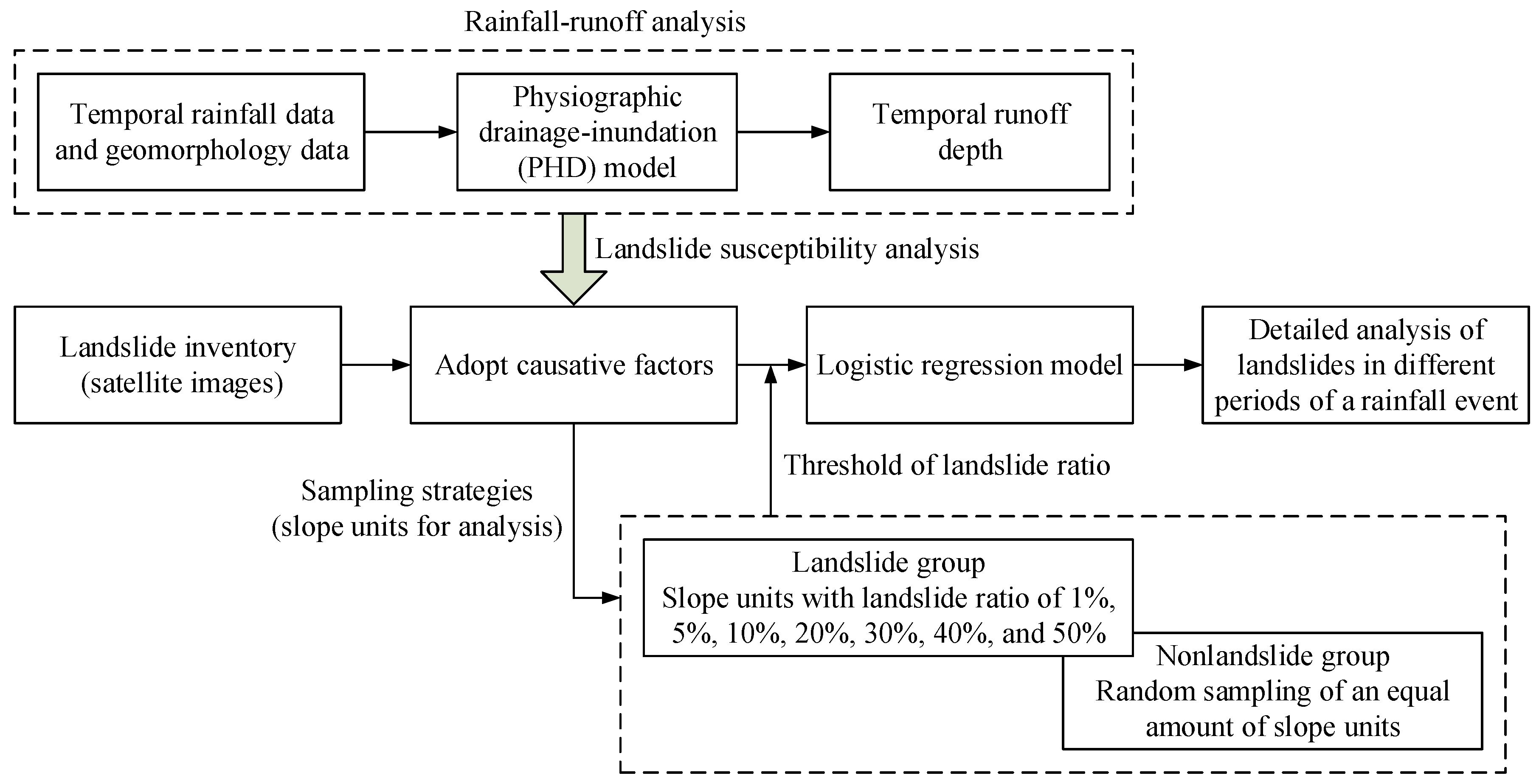
2.4. Rainfall-Runoff Model

The rainfall-runoff model adopted in this study was the physiographic drainage-inundation (PHD) model, which has been successfully applied to estimate rainfall runoff of various areas in Taiwan [21,22,23,24,25,26]. Conducting analysis with this model first involved categorizing the analysis areas by topography and water system. The present study used the GIS to divide the grids into slope grids and river grids and extracted the hydrological and physiographic data of the individual grids for rainfall-runoff analysis. Calculation of the PHD model was performed based on the continuity equation of flow and the flow law in each grid section. The model simulated the runoff flow across grid sections to identify runoff directions based on grid topography. The water level variations calculated through the water flow across the grids should satisfy the continuity equation of flow. Because the PHD model uses only a continuity equation to express variation in runoff flow, its estimation can be completed in a very short period. Hence, this model supports real-time prediction of the runoff amount generated in a rainfall event. The continuity equation of grid section i in the PHD model is expressed as follows [27]:

$$A_i\frac{\partial h_i}{\partial t}=P_{ei}(t)+{\displaystyle \sum _k{Q}_{i,k}(h_i,h_k)}$$

(1)

where $t$ is time; $A_i$ is the area of gird section i; $h_i$ and $h_k$ are the water level of grid sections i and k, respectively; $Q_{i,k}$ is the amount of water flowing from section k to an adjacent section i; and $P_{ei}$ is the effective rainfall volume in section i, which equals the product of the effective rainfall amount and the area of section i. Water flow across grid sections can be classified into river type and weir type. The calculation methods of various water flow types are illustrated as follows.

(1) River type

If no structure exists to obstruct water flow between two grids, the flow can be regarded as overland flow or as exhibiting a river-type link. Water flow at the boundary of two grids is calculated using the Manning formula, which estimates average resistance. Taking grid section i as an example, the water flow from grid section k to grid section i is:

$$Q_{i,k}=\frac{h_k-h_i}{\left|h_k-h_i\right|}\cdot \varphi ({\overline{h}}_{i,k})\cdot \sqrt{\left|h_k-h_i\right|}\mathrm{for}\frac{\partial Q_{i,k}}{\partial h_i}\le 0$$

(2)

$$Q_{i,k}=\varphi ({\overline{h}}_{i,k})\cdot \sqrt{\left|h_k-h_i\right|}\mathrm{for}\frac{\partial Q_{i,k}}{\partial h_i}>0$$

(3)

where ${\overline{h}}_{i,k}$ is the water level at the boundary between grid sections i and k. In addition, ${\overline{h}}_{i,k}=\alpha h_k+(1-\alpha )h_i$, where $\alpha$ is the weighting factor between the two grids; ${\overline{h}}_{i,k}$ is obtained by performing linear interpolation between $h_i$ and $h_k$, and $\varphi (h)$ is:

$$\varphi (h)=\frac{\frac{1}{n}A(h)R^{2/3}(h)}{\sqrt{\Delta x}}$$

(4)

where $\Delta x$ is the center distance between grids i and k, n is the Manning’s roughness coefficient between the two grids, A is the flow area at the boundary, and R is the hydraulic radius.

(2) Weir type

If flow exchange between two grids is hindered by obstacles such as roads, embankment, or ridge footpaths, the boundaries are regarded as broad-crested weirs and the linking is referred to as a weir-type link. The flow at the boundary between two grids is calculated using a weir equation. Weir flows can be divided into free and submerged weir flows based on the water level upstream and downstream as well as the difference in weir crest height. The flow quantities of the weir type are calculated as follows:

Free weir flow

$$(h_i-Z_w)<\frac{2}{3}(h_k-Z_w)$$

(5)

$$Q_{i,k}={\mu }_{f}b\sqrt{2g}{(h_k-Z_w)}^{3/2}$$

(6)

Submerged weir flow

$$(h_i-Z_w)\ge \frac{2}{3}(h_k-Z_w)$$

(7)

$$Q_{i,k}={\mu }_{s}b\sqrt{2g}(h_i-Z_w){(h_k-h_i)}^{1/2}$$

(8)

In Equations (5) and (6), $Z_w$ is the weir crest elevation; b is the effective width of the weir crest, namely the boundary length of two adjacent grid sections; g is the gravitational acceleration; and ${\mu }_f$ and ${\mu }_s$ are the weir flow coefficients of free weir flow and submerged weir flow, respectively. Typically, ${\mu }_f$ ranges between 0.36 and 0.57, and ${\mu }_s$ is 2.6 times that of ${\mu }_f$ [28].

The flow quantities $Q_{i,k}$ of adjacent grids and the corresponding water levels of these grid sections ($h_i$ and $h_k$) are expressed in Equations (2), (3), and (5)–(8). Equation (1) can be expressed as follows by using the explicit difference method:

$$h_i^{m+1}=h_i^m+\frac{({\sum }_k{Q}_{i,k}^m+P_{ei}^m)}{A_i}\cdot \Delta t$$

(9)

where m is the known physical quantity at time point $t_m$, the superscript m + 1 is the water level of a specific grid at time point $t_{m+1}$, and ∆t is the time difference involved in the calculation. By means of the rainfall, hydrological, and physiographic data of the grids, the runoff in various grids at various time points can be obtained from Equation (9). The depth of runoff flow of a grid is defined as:

$$D_i=h_i-z_i$$

(10)

where $D_i$ is the water depth of grid i, and $z_i$ is the bed elevation of grid i.

Because the PHD model simulates runoff flow primarily through flow exchange at grid boundaries, the boundaries should be simple straight lines to enhance the accuracy of flow quantity estimation on the boundary. However, analysis units typically adopted in landslide susceptibility models, such as slope units and grid units, tend to have complicated and curved boundaries to ensure that their boundaries are consistent with the physical boundaries of the area under analysis [18]. Applying such grids for the PHD model analysis affects the stability of model calculation. In this study, the complexity of the topography in the study area entailed that the amount of hydrological and physiographic data to be processed in the model calculation was considerable. The study area was divided into several zones. Zoning of these areas was performed using a digital elevation model with a spatial resolution of 5 m × 5 m. River channels were then marked according to the river channel width identified using satellite images. Subsequently, zoning of slope areas was preformed using soil maps, land use maps, and road system areas of the study area. When zoning was complete, the sizes of the analysis grids in different zones were checked and adjusted. If the grids were excessively large, they would encompass a wide range of elevation and exhibit relatively great difference in topography, and thus further division would be required to render the grids representative in terms of elevation. By contrast, if the grid sections were excessively small or elongated, map layer data could not be extracted, or the simulation of water body exchange would become unstable in the model; this would warrant further consolidation of these grids. Figure 3 presents the calculation grids for the PHD model, which were divided by the topographical features of the study area. A total of 3211 grids were used (Figure 4), of which 189 and 3022 belonged to river grids and slope grids, respectively.

2.5. Logistic Regression Analysis

Logistic regression has been widely introduced to landslide studies in the last three decades. It can be employed to perform simple but accurate fitting of independent and dependent variables. In this study, logistic regression analysis was adopted to assess the relationship between the dependent variable (i.e., landslide occurrence or nonoccurrence) and independent variables (relevant factors of landslides). The logistic regression equations of landslide susceptibility analysis can be expressed as follows [11]:

$$P=\frac{1}{(1+e^{-\lambda })}$$

(11)

$$\lambda =\alpha +{\displaystyle \sum _{i=1}^k{\beta }_k{x}_{ki}}$$

(12)

where $\lambda$ represents the logit function values of specific slope units, $\alpha$ is the intercept of the model, $x_{ki}$ represents the values of specific landslide susceptibility factors, and ${\beta }_k$ represents the corresponding regression coefficient. Substituting the logit function values of specific analysis grids into Equation (11) obtained the landslide probability P of various analysis grids, namely the landslide susceptibility values.

Before estimating landslide susceptibility, the grids of the analysis areas must be divided by terrain mapping units (TMUs), in which natural boundaries formed by various surface features are adopted as grid boundaries. Common TMU subdivisions include topographic units, terrain units, slope units, administrative units, grid cells, and unique-condition units [1]. Regardless of TMU subdivisions, the objective is to attain the highest possible level of homogeneity within a subdivision and notable heterogeneity among all subdivisions [29]. The most frequently adopted TMU subdivisions are slope units and grid cells [1]. Previous landslide hazard research indicated that because slope units have complete terrain-based boundaries, the results of landslide susceptibility analysis can serve as a reference for slope hazard management for competent authorities [30]. The landslide susceptibility analysis performance of various TMUs found that slope units attained the most satisfactory outcomes [1]. Because previous studies have obtained favorable landslide hazard analysis results by using slope units, the present study adopted slope units as the analysis grids of landslide susceptibility.

2.6. Landslide Inventories

The landslide inventories were prepared through the following steps. The satellite images of various landslide sites were compared before and after typhoon events. This enabled mapping newly created landslides sites as well as existing landslide sites that had expanded after typhoon events, and stacking landslide areas with slope units to sort these units into those with and without landslides (i.e., a landslide group and nonlandslide group). However, larger landslide sites may span multiple slope units, and some sites may be located only on the margin of the slope units. To prevent insufficiently large landslide areas from causing categorization errors, a threshold value must be determined. In other words, we determined whether individual slope units belonged to the landslide group based on their landslide ratios (the proportion of the landslide area to the overall slope unit area). However, previous studies have not reached a consensus on the optimal landslide ratio threshold [30,31,32,33]. Therefore, in the present study, tests were conducted with landslide ratios of 1%, 5%, 10%, 20%, 30%, 40%, and 50%. The optimal threshold was determined by comparing the results and was adopted for subsequent landslide susceptibility analysis.

When conducting the analysis for threshold selection, areas with slope gradients of <10% were considered as stable areas, whereas those with slope gradients of ≥50% were considered as hazardous areas for rockfalls [14]. Accordingly, areas with slope gradients of <10% and >50% were excluded from the nonlandslide group. The grouping results of both typhoon events revealed that regardless of the thresholds selected, the nonlandslide group contained far more slope units than did the landslide group. Therefore, if all slope units in the nonlandslide group were included in the landslide susceptibility analysis, the accuracy of this group would be exceptionally high, whereas that in the landslide group would be notably low, resulting in biases in the analysis results. Hence, the landslide susceptibility analysis included all slope units in the landslide group and an equal amount of slope units in the nonlandslide group. The selection process of the nonlandslide group consisted of 50 random samplings.

Table 2. List of the thresholds and the statistics of corresponding estimation accuracy.

Landslide Ratio (%)	Typhoon Talim				Typhoon Jangmi
	Overall Accuracy (%)	Mean	Standard Deviation	Slope Units for Landslide Group	Estimation Accuracy (%)	Mean	Standard Deviation	Slope Units for Landslide Group
1	69.5~75.1	71.5	1.6	211	74.4~82.5	78.4	1.8	160
5	70.1~79.3	74.1	2.0	167	77.6~85.8	81.7	1.6	123
10	69.8~79.4	74.7	2.1	131	73.8~87.6	81.5	2.4	101
20	68.9~81.1	73.8	2.7	106	79.7~88.5	83.8	2.1	74
30	68.1~81.9	75.3	2.7	80	78.4~90.2	85.6	2.6	51
40	67.2~82.1	74.0	4.0	67	76.3~91.3	84.6	3.4	40
50	69.4~88.9	78.5	4.1	54	75.0~96.2	86.1	5.0	26

presents the grouping results of various thresholds and the statistics for corresponding estimation accuracy.

The results of two typhoon events indicated that higher landslide ratios correspond to higher levels of model estimation accuracy. However, the available amounts of landslide group slope units were limited. The data of landslide ratio, mean accuracy, and landslide group slope units in Figure 5 show that for both Typhoon Talim and Typhoon Jangmi, the estimation accuracy and number of landslide group slope units intersected at a landslide ratio of 10–20% (inclining toward 20%). Thus, the landslide ratio of 20% was selected as the threshold to distinguish the landslide group in the study.

2.7. Factors of Landslide Susceptibility Model

A previous study indicated that numerous factors may influence landslides in the Alishan area, including elevation, slope gradient, terrain roughness, slope roughness, profile curvature, lithology, aspect, rainfall intensity, and slope height [25]. Because predicted runoff entailed the characteristics of rainfall and some topographical factors, this study simplified factors in subsequent landslide susceptibility analysis. Specifically, only aspect and slope gradient were retained and adopted alongside the estimated depth of runoff flow to perform the landslide susceptibility analysis. To prevent a single factor from affecting the simulation results with a distinctly different value range, the factors were normalized prior to landslide susceptibility analysis. The preparations of the adopted factors are as follows:

(1) Aspect

Aspect refers to a slope’s inclination direction. A correlation was found between landslide distribution area and aspect [34]. Aspect reflects the extent to which the slope is windward or leeward in a catchment area. Slopes with a windward aspect are more susceptible to erosion caused by torrential rain, which damages the soil structure and increases the probability of landslides. Therefore, aspect is considered a possible factor of landslides. In this study, aspect was calculated as a function of gradients at a given point on a surface [35]. The azimuth values of the slope units were calculated automatically using the spatial analysis module of the GIS. Aspect was then divided into nine types by using the obtained azimuth values.

(2) Slope gradient

Slopes with steeper gradients are subject to greater effects of gravitational force; these effects become the kinetic energy of the soil and rock in terms of slipping downward. Hence, slope gradient is often considered the most direct influencing factor of slope mechanics [1,5,11]. The present study adopted a spatial analysis module in the GIS to perform calculations on the topographical data in the 5 m × 5 m high-resolution digital elevation model (DEM). Zonal statistics were then used to extract the mean slope gradient of all slope units. The resulting slope gradient ranged from 1° to 66° in the study area.

(3) Depth of runoff flow

The temporal variations of runoff flow depth in the study area during rainfall were estimated by the PHD model. Because each slope unit contained multiple calculation grids in the PHD model, the mean water depth in an individual slope unit was adopted as the representative depth of runoff flow. Because the flow depth varies during rainfall with respect to rainfall amount and physiographic factors, analyzing this variable enables temporal variations in landslide susceptibility in the study area to be obtained at various time points during rainfall.

3. Results

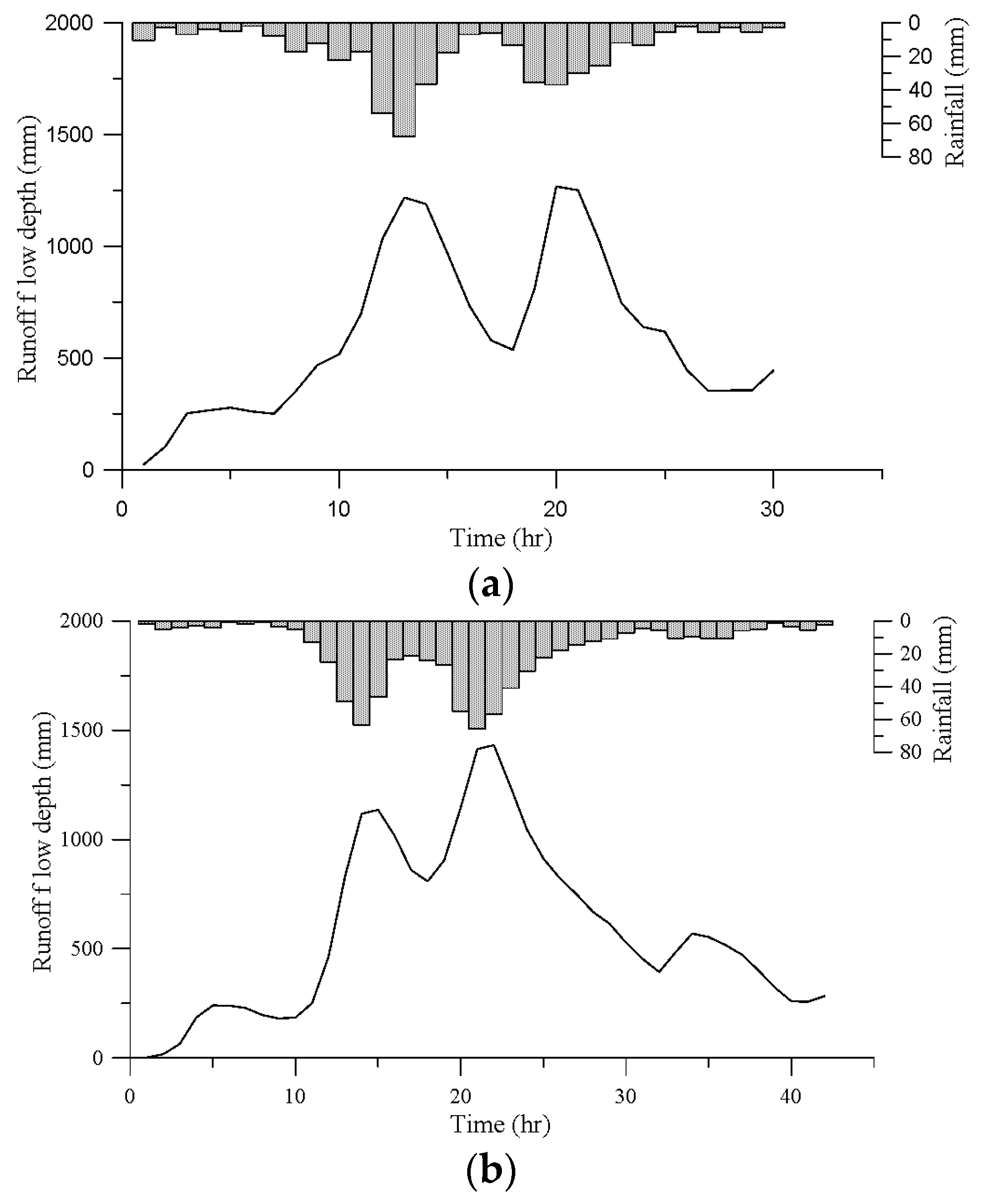
3.1. Rainfall-Runoff Analysis

Figure 6a,b present the simulated runoff flow depth and rainfall data during Typhoon Talim and Typhoon Jangmi, respectively. The runoff flow depth in the figure is represented by that of the slope unit at the outlet of the study area. Simulated values of runoff flow depth were plotted as line charts and the mean rainfall of the six rainfall stations during the typhoon periods were plotted as hydrographs. Figure 6a,b show that the variation trends of runoff flow depth and hourly rainfall were similar during the two typhoons. In the early stages of rainfall, because the runoff had not reached the outlet, the runoff flow depth maintained at a low value. When the rainfall duration and amount increased, the runoff flow depth increased significantly; when the rainfall duration and amount decreased, the runoff flow depth also decreased. The peak of overland flow depth occurred close to the peak of rainfall. The hydrograph of runoff flow faithfully reflects water level increases and decreases caused by rainfall variation. A comparison of the DEM and land use map of the study area showed that the runoff flows mostly occurred in low-lying areas of the slopes and areas with relatively low slope gradients near river channels. This indicated that the adopted PHD model can properly simulate changes in runoff flow due to terrain and land use in the study area. Therefore, substituting the factor of rainfall amount with runoff flow depth can more faithfully reflect the situations of water distribution. The PHD model simulation results were further assessed by comparing the results with the total rainfall volumes, which were obtained by adding the products of the rainfall amount at all rainfall stations and their control area.

Table 3. The comparison of the runoff volumes for different typhoon events.

Event	Simulations		Total Rainfall Volume (m3)	Runoff Error
	Total Outlet Discharge (m3)	Depression Storage (m3)
Typhoon Talim	34,944,289.2	1,011,033.8	36,376,655.0	1.16%
Typhoon Jangmi	48,230,661.6	556,015.3	49,276,512.2	0.99%

summarizes the total rainfall volume, total outlet discharge, and total depression storage. The simulation performance of the PHD model can be assessed in relation to runoff error (E_r), which is calculated as follows:

$$E_r=\frac{V_{\mathit{rainfall}}-(V_{\mathit{discharge}}+V_{depression})}{V_{\mathit{rainfall}}}$$

(13)

where $V_{\mathit{rainfall}}$ represents the total rainfall volume, $V_{\mathit{discharge}}$ represents the simulated discharge at the outlet, and $V_{depression}$ represents the simulated depression storage. The runoff error of Typhoon Talim was 1.16%, whereas that of Typhoon Jangmi was 0.99%. The runoff errors of both typhoons predicted by the PHD model were lower than 2.0%. These results indicated satisfactory conservation in the model calculation process. The PHD model was verified as reasonable and adequate for simulating rainfall runoff that occurred in areas of the Alishan River.

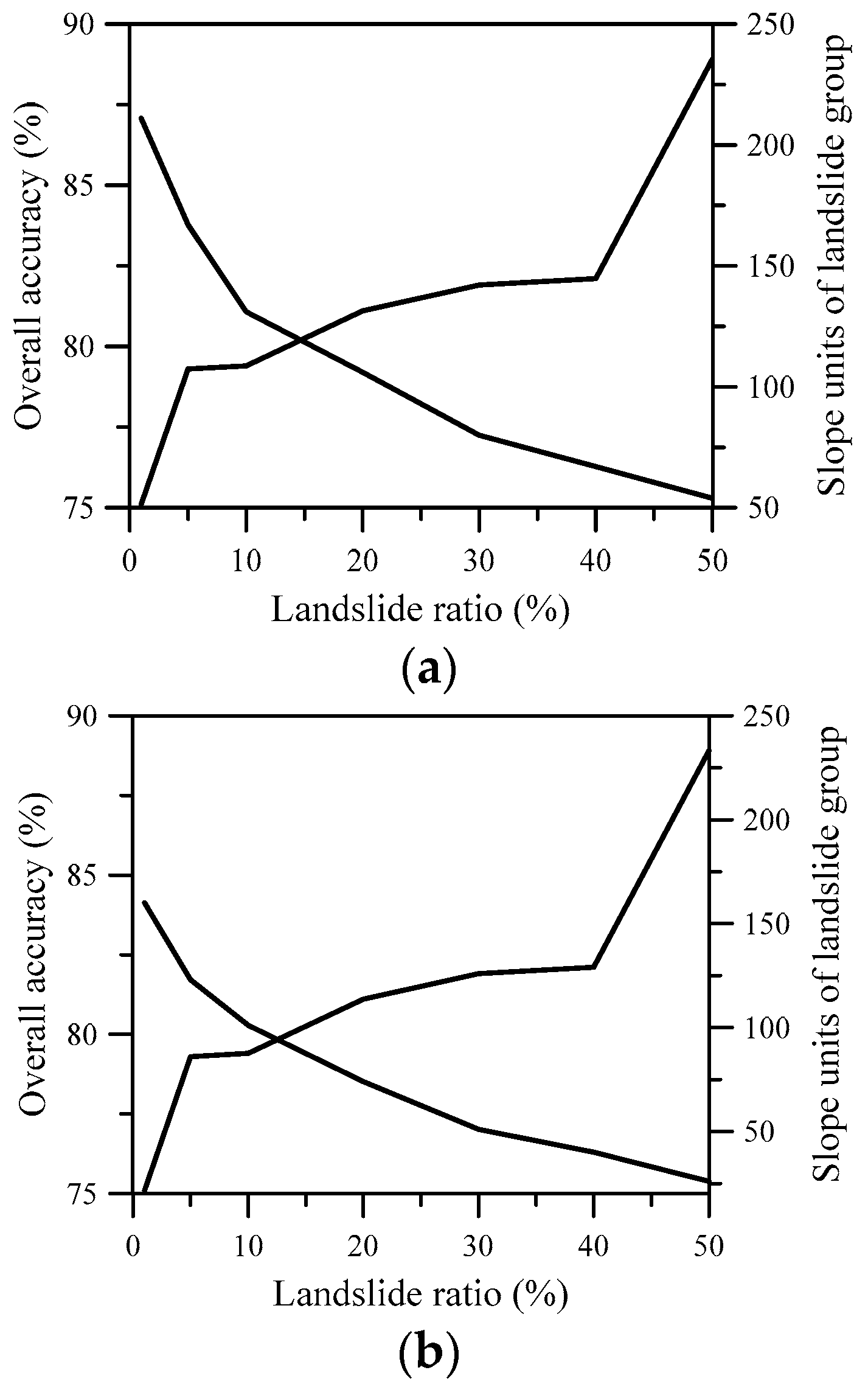
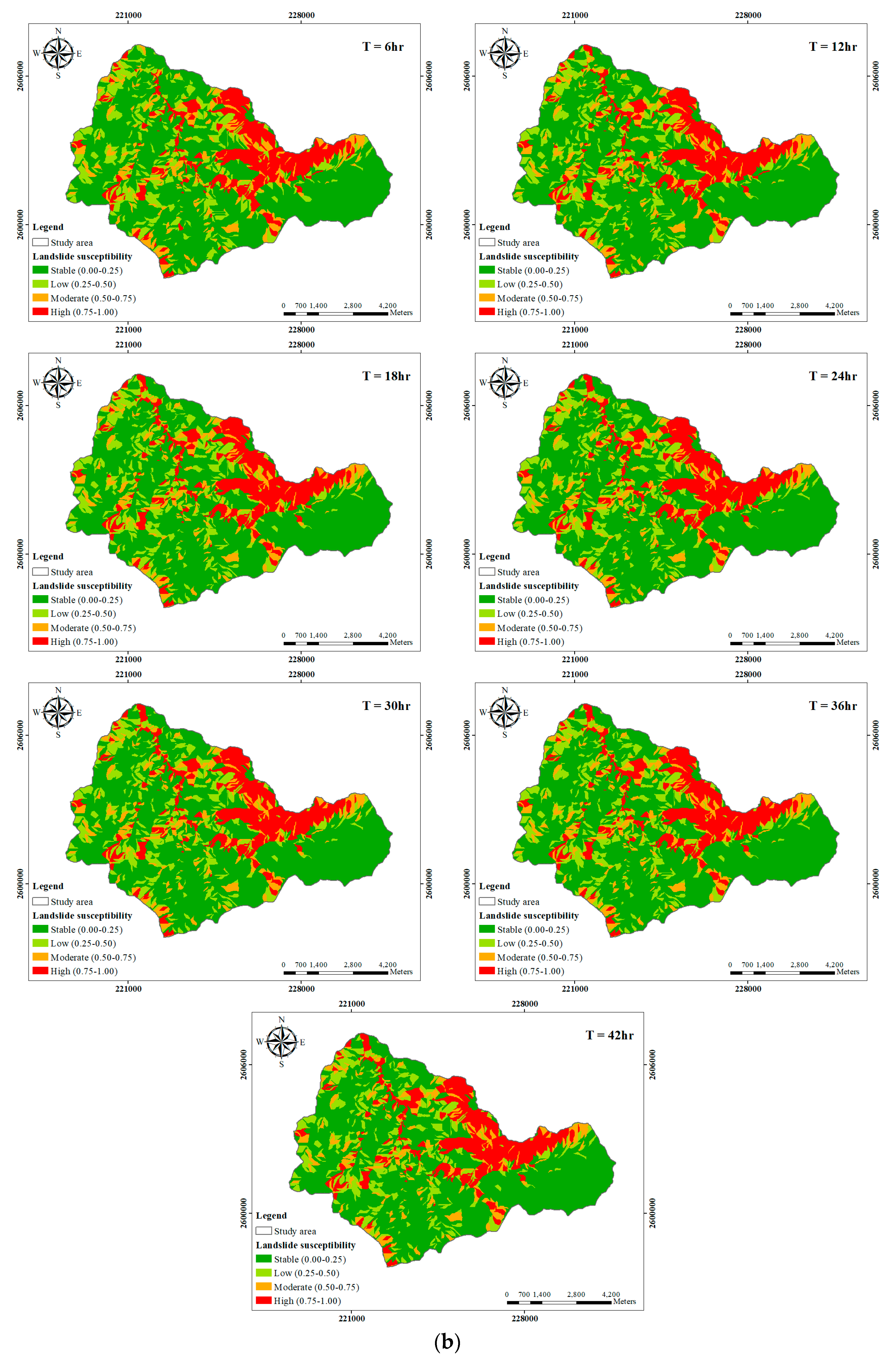
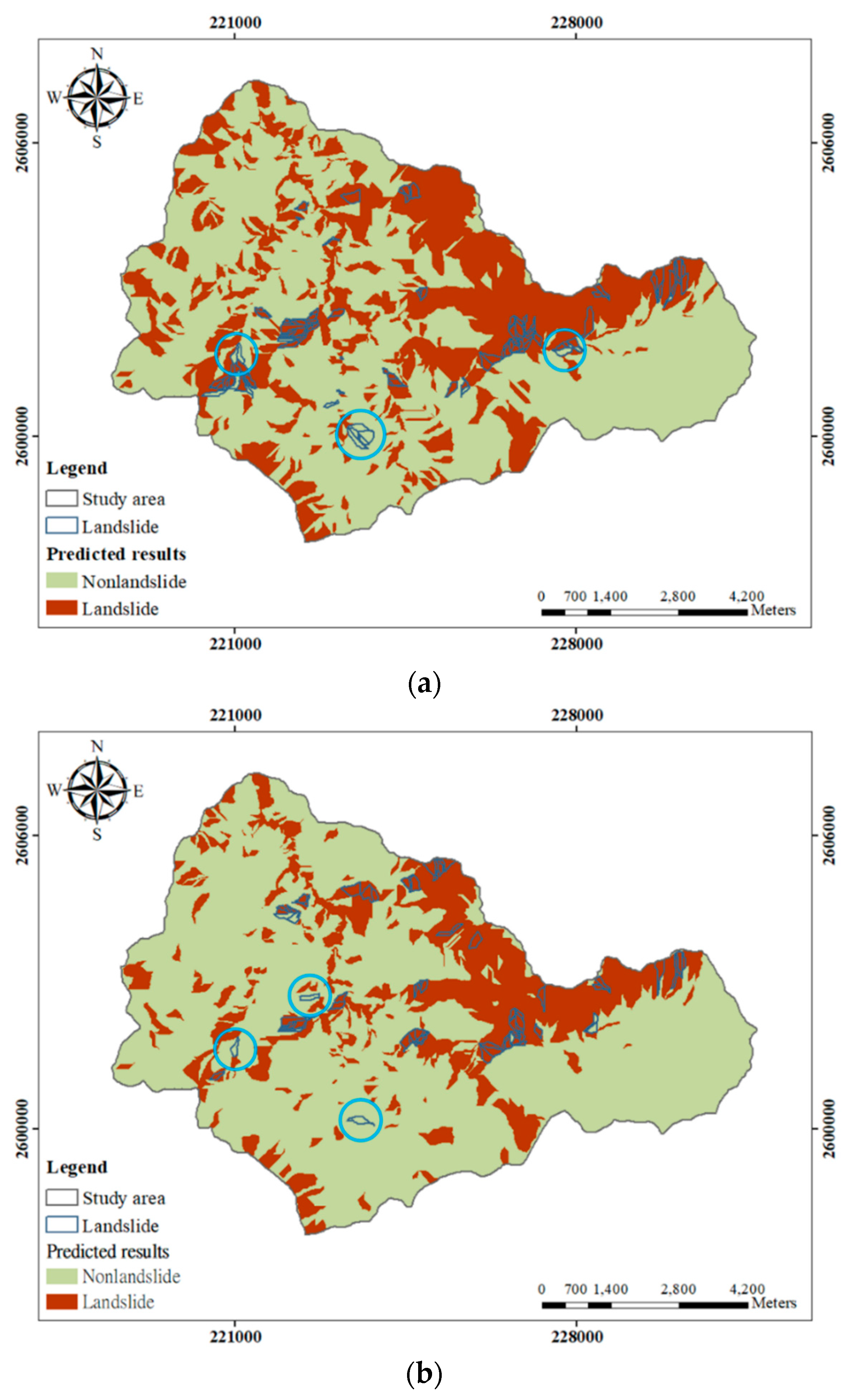
3.2. Landslide Susceptibility Analysis

Factors such as aspect, slope gradient, and runoff flow depth in various periods were input into the logistic regression model to obtain the regression coefficients. The results of logistic regression analysis are expressed as follows:

$$\begin{array}{ll}\lambda =& W_1\times L_1+W_2\times L_2+W_3\times L_3+W_4\times L_4+W_5\times L_5+W_6\times L_6+W_7\times L_7+W_8\times L_8\\ & +W_9\times L_9+W_{10}\times L_{10}+C\end{array}$$

(14)

where $W_1~W_{10}$ are the regression coefficients of various factors, C is the constant, $L_1~L_8$ are aspect values, $L_9$ is the slope value, and $L_{10}$ is the runoff flow depth, which changes throughout the rainfall process. In a logistic regression model, categorical variables must include indicator variables. The plane was adopted as the indicator aspect in this study. Each factor was standardized to the same scale before it was applied to the logistic regression analysis.

Table 4. Regression coefficients estimated for the logistic regression model.

Factor			Coefficient	Event
				Typhoon Talim	Typhoon Jangmi
Aspect	North	$L_1$	$W_1$	16.89~17.21	14.53~19.88
	Northeast	$L_2$	$W_2$	17.75~18.15	14.62~19.47
	East	$L_3$	$W_3$	18.19~18.46	16.09~20.51
	Southeast	$L_4$	$W_4$	18.44~19.00	15.85~19.93
	South	$L_5$	$W_5$	19.03~19.17	16.21~20.04
	Southwest	$L_6$	$W_6$	17.85~18.19	14.83~18.47
	West	$L_7$	$W_7$	18.34~18.57	15.09~18.62
	Northwest	$L_8$	$W_8$	17.98~18.31	13.95~16.18
Slope		$L_9$	$W_9$	1.71~1.83	2.54~3.16
Runoff depth		$L_{10}$	$W_{10}$	0.80~1.47	1.77~2.70
Constant		C	–	−18.82~−18.67	−20.39~−16.71

summarizes the regression coefficients of various factors throughout the rainfall periods of Typhoon Talim and Typhoon Jangmi. The regression coefficients revealed that aspect, slope gradient, and overland flow depth all positively correlated with landslide occurrence. The regression coefficient of aspect remained higher than those of the other two factors and the weight difference among various aspect values was minor. In Typhoon Talim, the regression coefficient of slopes with a southern aspect was slightly higher, whereas in Typhoon Jangmi, that of southern and eastern slopes were relatively high. This difference was a result of the two typhoon events having different visiting paths. Typhoon Talim moved from east to west, directly cutting through Taiwan; hence, it brought a southwestern monsoon that directly influenced southwestern Taiwan. Typhoon Jangmi made landfall in northeastern Taiwan and turned northward because of Taiwan’s terrain, and thus exerted less influence on central and southern Taiwan with a southwestern monsoon. Assessment of the landslide susceptibility prediction results was conducted using the classification error matrix (CEM) [36] and the area under a receiver operating characteristic curve (AUC) [37].

Table 5. The performance of the landslide susceptibility model. CEM = classification error matrix; AUC = area under a receiver operating characteristic curve.

Assessments		Event
		Typhoon Talim	Typhoon Jangmi
CEM (%)	For nonlandslide group	79.2~81.1	83.8~90.5
	For landslide group	80.2~83.0	85.1~87.8
	Overall accuracy	79.7~82.1	85.1~89.2
AUCs		0.771~0.795	0.838~0.876

shows that the AUC of all variables was higher than 0.7 and the CEM accuracy of most variables was higher than 80%, indicating that runoff flow depth, aspect, and slope gradient all achieved satisfactory results in landslide susceptibility analysis [38].

4. Discussion

The landslide susceptibility values in the study area were divided into four levels, including stable (0~0.25), low landslide susceptibility (0.25~0.5), moderate landslide susceptibility (0.5~0.75), and high landslide susceptibility (0.75~1). Figure 7a,b, respectively, illustrate the landslide susceptibility levels in various periods during the two typhoons. For Typhoon Talim, the stable area ranged between 35.10% and 37.82%, the low landslide susceptibility area ranged between 27.92% and 29.38%, the moderate landslide susceptibility area ranged between 17.28% and 18.85%, and the high landslide susceptibility area ranged between 15.53% and 17.11%. The prediction results revealed that the stable area and low landslide susceptibility area comprised most of the study area. Regarding the prediction results of Typhoon Jangmi, the stable area ranged between 51.82% and 61.12%, accounting for approximately half of the total area; the low landslide susceptibility area ranged between 13.89% and 16.73%; the moderate landslide susceptibility area ranged between 8.37% and 11.88%; and the high landslide susceptibility area ranged between 15.43% and 19.58%. The rainfall amount and duration of Typhoon Talim were smaller than those of Typhoon Jangmi; however, the mean rainfall intensity of Typhoon Talim was higher than that of Typhoon Jangmi. Because Typhoon Talim brought substantial rainfall within a short period, the landslide probability in the research site increased, expanding the moderate and high landslide susceptibility areas. Thus, for Typhoon Talim, the stable area accounted for a far smaller area than that for Typhoon Jangmi. In addition, the landslide susceptibility analysis adopted runoff flow depth as the influencing factor; this factor changes dynamically during the rainfall process. Thus, the proposed analysis method can be applied to predict the time point of landslide occurrence when similar rainfall events occur.

Using the time points at which Typhoon Talim and Typhoon Jangmi exhibited the most favorable overall accuracy as an example, the comparisons of real landslide and predicted landslide areas were shown in Figure 8a,b, considering a cut-off value of 0.5 to distinguish the susceptibilities into landslide and nonlandslide areas. The predicted results were approximately consistent with the actual landslide areas. The results indicated that the landslides in the study area were concentrated in the northeast, whereas a small proportion of them were scattered around the remainder of the study area. The reason for such a distribution pattern was that the southern slopes were located on the windward side during both typhoons, and most northeastern slopes in the study area have a southern or southwestern aspect, which renders them particularly susceptible to torrential rain and strong wind. The prediction results reflect the influence of aspect on the stability of slopes in the study area. However, the model did not accurately predict landslides with a western or northwestern aspect and those with a slope gradient of lower than 30° (marked by circles). The logistic regression model adopted the southern aspect as the main area of landslide occurrence and the slope gradient positively correlated with the probability of landslide occurrence. Therefore, the model was unable to predict landslide areas with a western aspect and a relatively low slope gradient. To improve the model accuracy, the study area could be further divided into a smaller scale for simulations, or alternatively, detailed landslide susceptibility and variation analysis could be performed on specific local areas of slopes in hazardous areas.

5. Conclusions

This study adopted the upstream area of the Alishan River in southern Taiwan as the study area to analyze the temporal variations of landslide susceptibility. A new landslide analysis procedure was established by combining the rainfall–runoff model and landslide susceptibility model. The results indicated that based on the runoff flow depth, aspect and slope gradient can serve as the factors of landslide susceptibility analysis. The landslide susceptibility model established using logistic regression can be used to analyze temporal variations among landslides caused by rainfall. Using runoff flow depth as an analysis factor can reduce the number of factors and enhance the data processing efficiency of the landslide susceptibility model. The model prediction results revealed that the substantial rainfall in a short period increased the landslide occurrence of the study area, thereby decreasing the proportion of stable areas. A comparison of landslide susceptibility variation during the typhoons revealed that the proposed analysis model can predict variations in landslide susceptibility caused by typhoon rainfall. The prediction results indicated that the landslide analysis process demonstrated accurate predictions. If rainfall prediction data are integrated in the future, the proposed rainfall–runoff model used alongside a landslide susceptibility analysis process can predict the time points of landslide occurrence, thereby providing new types of landslide data that the government can use to implement resident evacuation and road closure procedures. This study used event-type landslide data (landslides after a rainfall event) as a basis for landslide analysis. Temporal variations of landslide during a rainfall event can help to further verify the proposed model.

References

1. Guzzetti, F.; Carrara, A.; Cardinali, M.; Reichenbach, P. Landslide hazard evaluation: A review of current techniques and their application in a multi-scale study, Central Italy. Geomorphology 1999, 31, 181–216. [Google Scholar] [CrossRef]
2. Caine, N. The rainfall intensity-duration control of shallow landslides and debris flows. Geogr. Ann. Ser. A Phys. Geogr. 1980, 62, 23–27. [Google Scholar]
3. Atkinson, P.M.; Massari, R. Generalised linear modelling of susceptibility to landsliding in the central Apennines, Italy. Comput. Geosci. 1998, 24, 373–385. [Google Scholar] [CrossRef]
4. Bai, S.B.; Wang, J.; Lu, G.N.; Zhou, P.G.; Hou, S.S.; Xu, S.N. GIS-based logistic regression for landslide susceptibility mapping of the Zhongxian segment in the Three Gorges area, China. Geomorphology 2010, 115, 23–31. [Google Scholar] [CrossRef]
5. Dai, F.C.; Lee, C.F. Landslide characteristics and slope instability modeling using GIS, Lantau Island, Hong Kong. Geomorphology 2002, 42, 213–228. [Google Scholar] [CrossRef]
6. Dai, F.C.; Lee, C.F. A spatiotemporal probabilistic modelling of storm-induced shallow landsliding using aerial photographs and logistic regression. Earth Surf. Process. Landf. 2003, 28, 527–545. [Google Scholar] [CrossRef] [Green Version]
7. Dai, F.C.; Lee, C.F.; Li, J.; Xu, Z.W. Assessment of landslide susceptibility on the natural terrain of Lantau Island, Hong Kong. Environ. Geol. 2001, 40, 381–391. [Google Scholar]
8. Guns, M.; Vanacker, V. Logistic regression applied to natural hazards: Rare event logistic regression with replications. Nat. Hazards Earth Syst. Sci. 2012, 12, 1937–1947. [Google Scholar] [CrossRef]
9. Jade, S.; Sarkar, S. Statistical models for slope instability classification. Eng. Geol. 1993, 36, 91–98. [Google Scholar] [CrossRef]
10. Lee, S.; Min, K. Statistical analysis of landslide susceptibility at Yongin, Korea. Environ. Geol. 2001, 40, 1095–1113. [Google Scholar] [CrossRef]
11. Ohlmacher, G.C.; Davis, J.C. Using multiple logistic regression and GIS technology to predict landslide hazard in northeast Kansas, USA. Eng. Geol. 2003, 69, 331–343. [Google Scholar] [CrossRef]
12. Van Den Eeckhaut, M.; Vanwalleghem, T.; Poesen, J.; Govers, G.; Verstraeten, G.; Vandekerckhove, L. Prediction of landslide susceptibility using rare events logistic regression: A case-study in the Flemish Ardennes (Belgium). Geomorphology 2006, 76, 392–410. [Google Scholar] [CrossRef]
13. Koukis, G.; Ziourkas, C. Slope instability phenomena in Greece: A statistical analysis. Bull. Int. Assoc. Eng. Geol. 1991, 43, 47–60. [Google Scholar] [CrossRef]
14. Chan, H.C.; Chang, C.C.; Chen, S.C.; Wei, Y.S.; Wang, Z.B.; Lee, T.S. Investigation and Analysis of the Characteristics of Shallow Landslides in Mountainous Areas of Taiwan. J. Chin. Soil Water Conserv. 2015, 46, 19–28. (In Chinese) [Google Scholar]
15. Central Weather Bureau, Taiwan, 2017: Records of Historical Typhoons. Available online: http://www.cwb.gov.tw (accessed on 12 June 2018). (In Chinese)
16. Pradel, D.; Raad, G. Effect of permeability on surficial stability of homogeneous slopes. J. Geotech. Eng. 1993, 119, 315–332. [Google Scholar] [CrossRef]
17. Guzzetti, F.; Peruccacci, S.; Rossi, M.; Stark, C.P. The rainfall intensity–duration control of shallow landslides and debris flows: An update. Landslides 2008, 5, 3–17. [Google Scholar] [CrossRef]
18. Shou, K.J.; Yang, C.M. Predictive Analysis of Landslide Susceptibility under Climate Change Conditions—A Study on the Chingshui River Watershed of Taiwan. Eng. Geol. 2015, 192, 46–62. [Google Scholar] [CrossRef]
19. Tseng, C.M.; Chen, Y.R.; Wu, S.M. Scale and spatial distribution assessment of rainfall-induced landslides in a catchment with mountain roads. Nat. Hazards Earth Syst. Sci. 2018, 18, 687–708. [Google Scholar] [CrossRef]
20. Chow, V.T.; Maidment, D.R.; Mays, L.W. Applied Hydrology; McGraw-Hill: New York, NY, USA, 1988. [Google Scholar]
21. Chen, C.N.; Tfwala, S.S. Impacts of Climate Change and Land Subsidence on Inundation Risk. Water 2018, 10, 157. [Google Scholar] [CrossRef]
22. Chen, C.N.; Tsai, C.H. The Impact of Climate Change on Inundation Potential. Int. J. Environ. Sci. Dev. 2013, 4, 496–500. [Google Scholar] [CrossRef]
23. Chen, C.N.; Tsai, C.H.; Tsai, C.T. Simulation of sediment yield from watershed by physiographic soil erosion–deposition model. J. Hydrol. 2006, 327, 293–303. [Google Scholar] [CrossRef]
24. Chen, C.N.; Tsai, C.H.; Tsai, C.T. Reduction of discharge hydrograph and flood stage resulted from upstream detention ponds. Hydrol. Process. 2007, 21, 3492–3506. [Google Scholar] [CrossRef]
25. Chen, S.C.; Chang, C.C.; Chan, H.C.; Huang, L.M.; Lin, L.L. Modeling typhoon event-induced landslides using GIS-based logistic regression: A case study of Alishan Forestry Railway, Taiwan. Math. Prob. Eng. 2013. [Google Scholar] [CrossRef]
26. Shiau, J.T.; Chen, C.N.; Tsai, C.T. Physiographic drainage-inundation model based flooding vulnerability assessment. Water Resour. Manag. 2012, 26, 1307–1323. [Google Scholar] [CrossRef]
27. Cunge, J.A. Unsteady Flow in Open Channel; Water Resources Publishing Limited: London, UK, 1980. [Google Scholar]
28. Tsai, C.T.; Tsai, C.H. A study on the applicability of discharge formulas for trapezoidal broad-crested weirs. J. Taiwan Water Conserv. 1997, 45, 29–45. (In Chinese) [Google Scholar]
29. Hansen, A. Landslide hazard analysis. In Slope Instability; Brunsden, D., Prior, D.B., Eds.; John Wiley and Sons: New York, NY, USA, 1984; pp. 523–602. [Google Scholar]
30. Carrara, A. Multivariate models for landslide hazard evaluation. J. Int. Assoc. Math. Geol. 1983, 15, 403–426. [Google Scholar] [CrossRef]
31. Erener, A.; Düzgün, H.S.B. Landslide susceptibility assessment: What are the effects of mapping unit and mapping method? Environ. Earth Sci. 2012, 66, 859–877. [Google Scholar] [CrossRef]
32. Guzzetti, F.; Reichenbach, P.; Cardinali, M.; Galli, M.; Ardizzone, F. Probabilistic landslide hazard assessment at the basin scale. Geomorphology 2005, 72, 272–299. [Google Scholar] [CrossRef]
33. Rossi, M.; Guzzetti, F.; Reichenbach, P.; Mondini, A.C.; Peruccacci, S. Optimal landslide susceptibility zonation based on multiple forecasts. Geomorphology 2010, 114, 129–142. [Google Scholar] [CrossRef]
34. Pearce, A.J.; O’Loughlin, C.L. Landsliding during a M 7.7 earthquake: Influence of geology and topography. Geology 1985, 13, 855–858. [Google Scholar] [CrossRef]
35. Wilson, J.P.; Gallant, J.C. (Eds.) Terrain Analysis: Principles and Applications; John Wiley and Sons: New York, NY, USA, 2000; pp. 51–86. [Google Scholar]
36. Lillesand, T.M.; Kiefer, R.W. Remote Sensing and Image Interpretation; Wiley and Sons: New York, NY, USA, 2000. [Google Scholar]
37. Begueria, S. Validation and evaluation of predictive models in hazard assessment and risk management. Nat. Hazards 2006, 37, 315–329. [Google Scholar] [CrossRef] [Green Version]
38. Swets, J.A. Measuring the accuracy of diagnostic systems. Science 1988, 240, 1285–1293. [Google Scholar] [CrossRef] [PubMed]
Figure 1. The flowchart of this study.
Water 10 01354 g001
Figure 2. Location of study area in the upstream area of the Alishan River.
Water 10 01354 g002
Figure 3. Control area and rainfall hyetograph of each rainfall station.
Water 10 01354 g003
Figure 4. Distributions of the calculation grids for the PHD model analysis.
Water 10 01354 g004
Figure 5. Variations of mean accuracy with slope units of landslide group and landslide ratio: (a) Typhoon Talim and (b) Typhoon Jangmi.
Water 10 01354 g005
Figure 6. Simulation results of runoff at the outlet of the study area and the corresponding rainfall: (a) Typhoon Talim and (b) Typhoon Jangmi.
Water 10 01354 g006
Figure 7. Variations of predicted susceptibility levels with respect to the rainfall durations: (a) Typhoon Talim and (b) Typhoon Jangmi.
Water 10 01354 g007aWater 10 01354 g007b
Figure 8. Resultant maps of landslides triggered by typhoon rainfall: (a) T = 24 h at Typhoon Talim and (b) T = 20 h at Typhoon Jangmi.
Water 10 01354 g008