Abstract
The influence of initial state variables on flood forecasting accuracy by using conceptual hydrological models is analyzed in this paper and a novel flood forecasting method based on correction of initial state variables is proposed. The new method is abbreviated as ISVC (Initial State Variable Correction). The ISVC takes the residual between the measured and forecasted flows during the initial period of the flood event as the objective function, and it uses a particle swarm optimization algorithm to correct the initial state variables, which are then used to drive the flood forecasting model. The historical flood events of 11 watersheds in south China are forecasted and verified, and important issues concerning the ISVC application are then discussed. The study results show that the ISVC is effective and applicable in flood forecasting tasks. It can significantly improve the flood forecasting accuracy in most cases.
1. Introduction
Conceptual hydrological models are widely applied in flood forecasting at present [1,2]. It is usually considered that flood forecasting errors come from five aspects: (i) model input; (ii) model structure; (iii) model parameters; (iv) measured data; and (v) initial state variables.
Model inputs mainly include rainfall and potential evapotranspiration. The rainfall commonly used in conceptual hydrological modelling is the basin average rainfall, which is calculated through the weighted average method. Reasonable density and location of rainfall stations can ensure good representativeness and accuracy of mean areal rainfall, especially with the assistance of auxiliary rainfall radar and satellite remote sensing precipitation technology, which is expected to further improve the observation accuracy of precipitation [3,4,5]. However, absolutely accurate rainfall measurement remains a difficult problem because of many impact factors such as the inhomogeneity of the spatial-temporal distribution of the rainfall, the variability of local micro climate and topography, the accuracy of gauge measurement, communication status of telemetry stations, and so on. Therefore, in traditional flood forecasting, rainfall observation error cannot be avoided by only using the method of calculating mean areal rainfall based on rainfall gauges.
The potential evapotranspiration used in conceptual models is usually substituted by surface evaporation measured with an evaporating dish for the sake of applicability and simplicity. The average evaporation of a basin is calculated by using multiple-point evaporation observation, which is similar to the calculation principle of rainfall. Compared with rainfall stations, the density of evaporation stations is sparse. It is specified in “Technical Guidelines for Hydrological Network Planning SL34-92” in China [6] that the control area of a single evaporation station should be between 2500 km2 and 5000 km2. Many small- and medium-sized basins have an area of about 1000 km2 and there is no evaporation station. This situation means that only evaporation data from nearby evaporation stations have to be transferred to the studied basin and are used for flood forecasting. Even worse, the collected data of evaporation are often scarce and real-time evaporation data can hardly be collected, and, on the contrary, only historical average evaporation data can be used as a model input for real-time flood forecasting. The above-mentioned conditions certainly lead to estimation error in the amount of evaporation. The solution of this problem lies in the increasing of the evaporation station density. However, it usually leads to higher costs and poorer economic benefits.
The conceptual model is based on experts’ understanding of hydrological laws. Hydrologists set up model structures to simulate hydrological processes and the model structures are based on the mathematical equations and the model parameters [7,8]. Since the hydrological processes cannot be well simulated solely based on physical basis at present, the structure of the hydrological model cannot fully reflect the law of hydrological process. Therefore, there are model structure errors in hydrological models. Conceptual models include the Xinanjiang model, the Tank model, and the Sacramento model, etc. The Xinanjiang model is proposed by Renjun Zhao in 1973 [9] and widely used in China [10,11,12]. Tank model is another conceptual model developed in Japan [13]. With further understanding of hydrological processes, conceptual models are also evolving. For example, along with the development of hillslope hydrology, the runoff components separation module of the Xinanjiang hydrological model has been developed from the initial two runoff components to the three runoff components [14]. The model structure is the core of the model; however, the development of hydrological models is very difficult. It embodies great efforts and wisdoms of a large number of hydrological scientists. It is not easy to develop a hydrological model with better versatility and higher accuracy [15,16].
The parameters of conceptual models have a physical basis to some extent, but the physical meanings of some parameters are not robust enough and therefore cannot be directly derived by observation and measurement. They can only be estimated using historical hydro-meteorological data by means of parameter calibration [17]. Genetic algorithm [18], SCE-UA method [19] and particle swarm optimization [20,21] are often used for parameter calibration. The estimated parameters are only a comprehensive reflection of information contained in historical data and may not clearly represent the characteristics of future flood events. Therefore, there are parameter errors in conceptual models that the reliability and representativeness can only be improved by using as many historical data as possible.
The measured flow is not only the important objective information of the model parameter calibration, but also the validation standard for the accuracy evaluation of flood forecasting. For the natural river, there are errors contained in the measured flow data because of the limitation of measurement technology. The errors can be reduced by using more advanced observation equipment [22], but will lead to higher costs. For the reservoir, the measured flow is usually obtained by conversion method from the reservoir water level. However, there are often errors because of the errors contained in reservoir water level data and various conversion curves [23].
To summarize, it takes high economic, labor, and time costs to improve the flood forecasting accuracy by focusing on model inputs, structure, parameters, and measured flow. These methods are difficult and uneconomic to apply. Therefore, we study the impact of state variables on flood forecasting, and summarize the shortcomings of the existing error correction methods of state variables, and finally try to propose a more efficient and effective state variables correction method.
State variables, such as soil moisture, proportion of runoff generation area, and free water depth, vary with time in the conceptual model. The state variables are calculated by model input and model parameters. According to the model structure design, some state variables have tiny influence on the results of subsequent calculations, while other state variables, which change over time and cause error accumulation, have significant impacts on the subsequent calculations. Because of the error of model inputs and parameters, there is error in state variables. Especially with the process of calculation, the cumulative errors of state variables will gradually increase. For flood forecasting, the initial state variables have large effects and impacts. Therefore, some scholars devote themselves to the study of state variables correction. Weerts used sequential importance resampling (SIR) filter, residual resampling filter (RR) and an ensemble Kalman (EnKF) filter to correct state variables. The results show that EnKF performs best with a low number of ensemble members [24]. Komma updated soil moisture of a distributed rainfall runoff model in forecasting large floods by Ensemble Kalman Filter and the results indicated that the updating procedure indeed improved the forecasts substantially [25]. The effect of initial state variables can be explained by Xinanjiang model herein. The Xinanjiang model is a famous conceptual hydrological model that is applicable in humid and semi-humid areas, and has been successfully and widely used all over the world [26].
The Xinanjiang model is a semi-distributed model. Usually, the basin is divided into several blocks according to the number and location of the rainfall stations, the river shape and the topography. Each sub-block uses the Xinanjiang model to calculate the flow process at the outlet section of the river basin, and the calculation flow of the whole basin is obtained by adding the flow of each sub-block above. In order to facilitate the calculation process and the determination of the parameters, all the parameters of the Xinanjiang model in each sub-block, except for n, are the same. The structure diagram of the Xinanjiang model is shown in Figure 1. All symbols inside the blocks are state variables, all symbols outside the blocks are parameters and the physical meaning of these parameters are shown in Table 1.
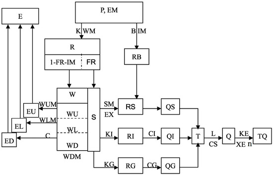
Figure 1.
Structure diagram of the three runoff components of the Xinanjiang model.

Table 1.
Parameters of the Xinanjiang model.
In Figure 1, there are seven state variables, including tension water content of upper soil layer (WU), lower soil layer (WL), deep soil layer (WD), proportion of runoff generation area (FR), free water storage (S), interflow runoff (QI), and groundwater runoff (QG), which have impact on subsequent flood forecasting.
The soil layer is divided into upper, lower, and deep layers in the Xinanjiang model, and the soil moisture of each layer is a state variable that changes over time. The initial soil moistures WU, WL, and WD directly affect the calculation of the runoff (R) and the evapotranspiration (E). The proportion of runoff generation area (FR) is considered changing over time. Therefore, it is necessary to know the initial FR at the beginning of the calculation. The free water storage (S) is also changing over time, which affects the surface runoff (RS), the interflow (RI), and the groundwater runoff (RG). QI and QG are the flows converted from the runoff depths RI and RG. Initial QI and QG are needed when calculating the flow concentration of RI and RG, by the method of linear reservoir.
The ranges of the above seven state variables are shown in Table 2.

Table 2.
The ranges of state variables of the Xinanjiang model.
In flood forecasting, the initial state variables have significant impacts on the forecasting results. Taking the flood event during 29 August 2016 8:00 and 3 September 2016 8:00 in Liangjiang hydropower station as an example, we set the initial state variables (at 29 August 2016 8:00) as three scenarios including normal, dry, and fully saturated. The simulations of the Xinanjiang model are shown in Figure 2. The error statistics results are shown in Table 3. The initial state variables of three scenarios are shown in Table 4.
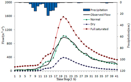
Figure 2.
Observed and simulated results using different initial state variables.

Table 3.
Error statistics of calculation results using different initial state variables.

Table 4.
The initial state variables of three scenarios.
As we can see in Figure 2, the influence of initial state variables on flood forecasting has two characteristics. One is systematic influence, that is, when the state variables become larger, the forecasting results become larger systematically and vice versa. The other is continuity influence, that is, adjusting the initial state variables will affect the following forecast results.
Although the state variables in the conceptual model have physical basis to some extent, the physical meanings of some state variables are still not strong and robust. Due to the limitations of observation techniques, many state variables lack the observed data to be validated. Therefore, the accuracy of the simulated state variables is difficult to judge. Set the Xinanjiang model as an example, the tension water storage (W) is used to describe the dynamic changes of soil moisture, which reflects the degree of wet and dry. However, the simulated W is usually not exactly consistent with the measured soil moisture [27,28]. Therefore, as a compromise, state variables are usually indirectly verified by streamflow forecasting accuracy because of lack of measured soil moisture data for direct verification. It is generally agreed when the forecasting results are accurate, the state variables are accurate too. On the contrary, when the forecasting results are inaccurate, the simulated state variables are recognized as unreliable.
At present, there are two main ways to adjust the initial state variables. One is manual adjustment at the beginning of the forecast. The state variables are adjusted manually according to the comparison results of the streamflow prediction. Manual adjustment, with large randomness and lack of standards, requires higher level of experiences for scientists and engineers. The other is to use the real-time correction method during the forecasting process for continuous dynamic adjustment, such as the commonly used Kalman filtering. With the residuals between the measured and forecasted flows, the Kalman filter uses the state and measurement equations to implement continuous correction of the state variables. However, the calculation process is complex, which needs the linearization of the hydrological model equations in the state space [29]. In addition, Kalman filtering requires continuous new information (usually real-time measured discharge) and is difficult to apply without real-time data scenarios.
Theoretically, the accuracy of flood forecasting can be remarkably improved by eliminating the above five kinds of errors. At present, there are many studies and countermeasures to reduce errors in the aspect of model input, model structure, model parameters, and measured flow data. However, there are few countermeasures to reduce the errors of initial state variables. In this paper, the influence of initial state variables on flood forecasting errors is studied, and countermeasures (Initial State Variable error Correction (ISVC) method) are developed to correct the initial state variables so as to improve the accuracy of flood forecasting. The ISVC method overcomes the shortcomings of the traditional manual correction of the initial state variables, and has the value of popularization and application. The famous conceptual hydrological model, the Xinanjiang model, is taken as an example. The proposed ISVC method is applied to 11 typical watersheds in humid regions of China, and obtains good flood forecasting results, which constructs a good foundation for further popularization and application of the ISVC method.
2. Methods
A typical flood forecasting process is shown in Figure 3. A flood forecasting process starts from the calculation start time to the calculation end time. The forecast start time is the start point of flood forecasting and is usually chosen after the main peak rainfall has appeared. The warm-up period is the period between the calculation begin time and the forecast start time. The measured flow is known during the warm-up period. Steady period, in which there is only slightly small rainfall, is the period from the calculation start time to the beginning of flood drastic rising (rising time) within the warm-up period. During the steady period, the main peak rainfall has not appeared, and the hydrograph is relatively flat.
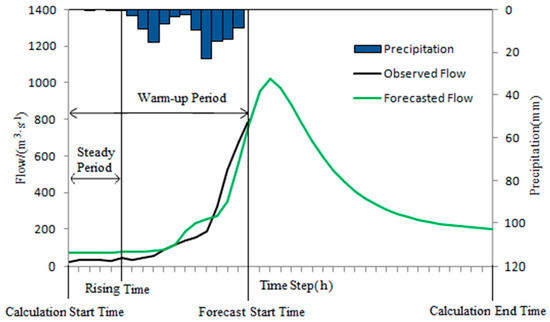
Figure 3.
A typical flood forecasting process.
Because the rainfall is very little during the steady period, the forecasted flow is mainly affected by the initial state variables, and the accuracy of the forecasted flow can significantly reflect the accuracy of the initial state variables. Therefore, the forecasted and measured flows during the steady period can be used as the input of automatic optimization algorithm to correct the initial state variables. Since the initial state variables have continuous and systematic impacts on the flood forecasting, when the steady period obtains good simulation results, the initial state variables can be considered accurate. That is, when forecasting results are good in steady period, the forecasting results are also usually more reliable in the whole flood event. Therefore, it is hoped that corrected initial state variables will improve flood forecasting accuracy. Based on the above principle, a new flood forecasting method is proposed, which is abbreviated as ISVC (Initial State Variable Correction) method.
The specific steps of the ISVC method are shown as follows:
- (1)
- Obtain the initial state variables by running the daily time-scale hydrological model (such as the Xinanjiang daily model) continuously and extract the initial state variables from the daily simulation results, or manually setting a set of proper initial state variables according to experience; and do initial flood forecasting.
- (2)
- Determine the steady period by observing the rainfall, the measured and forecasted hydrographs within the warm-up period;
- (3)
- Calculate the Normalized Root Mean Square Error (NRMSE) between the forecasted and measured hydrographs during the steady period, and determine whether it exceeds the predefined threshold. If so, go to step (4), otherwise, jump to step (7);
- (4)
- Calculate the deviation U between the forecasted and measured hydrographs during the steady period;
- (5)
- Determine the range of initial state variables according to U;
- (6)
- The optimization algorithm is used to find the optimal initial state variable values;
- (7)
- Do flood forecasting with the corrected initial state variables. If NRMSE exceeds the predefined threshold, go to step (4), otherwise, exit ISVC method.
The following Section 2.1, Section 2.2, Section 2.3, Section 2.4, Section 2.5 and Section 2.6 are the detailed explanations of the above-mentioned steps.
2.1. Steady Period Selection
Select the steady period manually. The steady period is from the calculation start time to the rising time. The rising time is selected before the measured and forecasted flows have not obviously risen, and at which the main peak rainfall has just started.
2.2. Normalized Root Mean Square Error
The formula of the normalized root mean square error (NRMSE) [30] is as follows:
where NRMSE is the normalized root mean square error, is calculated flow, is observed flow, is the average value of observed flow and is data sequence length.
When flood forecasting is error free, the value of NRMSE is 0. Given a threshold of NRMSE, the initial state variable does not need to be adjusted when the calculated error during steady period is within the threshold. When the NRMSE of steady period exceeds the threshold, the initial state variables are not correct and need to be adjusted. The threshold value will be further discussed in Section 4.1.
2.3. Deviation
Deviation [30] is used to measure the average systematic deviation of the forecasted flow from the measured flow. Calculation of deviation is shown in formula (2).
where the deviation U is the difference between the average value of calculated flow and the average value of observed flow, is the mean value of calculated flow, is the mean value of observed flow.
When U > 0, it means that the forecasted value is too large. When U < 0, it means that the prediction value is too small, and when U = 0 means the average system deviation is zero.
2.4. Correction of the Initial State Variables
Most modern conceptual hydrological models divide the whole basin into several sub-basins to consider the spatial inhomogeneity of hydrological variables. In order to consider the influence of spatial unevenness of the rainfall distribution, the basin needs to be divided into several blocks, and each block contains several rainfall stations, which respectively have their own weights to calculate mean areal rainfall. Each block has its own initial state variables, so there are multiple initial state variables. When applying the ISVC method, if initial state variables of each block are corrected separately, the workload will be greatly increased and the efficiency of the ISVC method will be affected due to too high dimensionality of the decision variables (usually recognized as the “dimensionality curse”). Therefore, a coefficient is given for each type of state variable, and then the coefficients are corrected. The initial state variables of each block are multiplied by the corresponding coefficients to obtain the corrected state variables. In this way, the number of parameters need correction is the number of initial state variables, which can greatly reduce the number of decision variables that need to be optimized and avoid the “dimensionality curse”.
Take the Xinanjiang model as an example. There are seven types of state variables, including WU, WL, WD, FR, S, QI, and QG, and these variables correspond to seven correction coefficients including , , , , , , and . The coefficients boundaries are shown in Table 5. When U > 0, the coefficients are less than 1 and the initial state variables will be reduced. When U < 0, the coefficients are larger than 1 and the initial state variables will be increased.

Table 5.
The boundaries of the coefficients of state variables.
Here, WUmin, WLmin, WDmin, FRmin, Smin, RImin and RGmin are minimum values of the initial state variables that are positive in all blocks. If the minimum value is 0, we set it to 0.01 to avoid errors in the calculation. When the corrected initial state variable value exceeds the upper boundary, set the state variable to its maximum value.
2.5. Objective Function
The absolute value of the error is used as the objective function. The formula is given by
where is observed flow, is calculated flow, is data sequence length and is weighting factor.
In order to emphasize new information of observed flow, set ,. Thus, the optimized state variables can reflect the basin state near the forecast start time better.
2.6. Optimization Algorithm
There are many optimization algorithms [31,32], such as genetic algorithm, particle swarm optimization (PSO), group compound evolution algorithm, fish swarm algorithm, simulated annealing algorithm, and ant colony algorithm. PSO [20], based on the simulation of bird prey behavior, is an intelligent swarm optimization algorithm proposed by Kennedy and Eberhart in 1995. If we consider an optimization problem in the air as foraging birds, a foraging bird flying in the air is a particle in the search space of the PSO algorithm, and the food position is the optimal solution to the optimization problem. The PSO algorithm belongs to evolutionary algorithms. It starts with a set of random solutions and finds the optimal solution iteratively. The quality of the solution is evaluated by the fitness value. Unlike genetic algorithms, PSO algorithm does not have operations such as “crossover” and “mutation”, and it is easy to find the global optimum by following the current search to the optimal value. PSO algorithm has attracted the attention of the academic community, and has demonstrated its superiority in solving practical problems because of its advantages of easy implementation, high precision, and fast convergence. Standard particle swarm optimization [21], is applied in this paper. Particle swarm size (M) is set to 70 and the number of particle dimensions (D) is 7, and D is same with the number of correction coefficients of the state variables. The values of the acceleration factors ( and ) are 2, the limit coefficient (K) between the position and the speed is 0.729, the value of adaptive inertia weight () is adjusted between 0.5 and 0.9, and the iterative termination condition, which is set as the difference between the two iterations of the objective function, is set to .
3. Materials
Eleven basins, located in Jiangxi and Zhejiang provinces, central southern China, are selected as the study areas. The areas of selected basins range from tens to thousands of square kilometers, and the research basins have both natural rivers and artificial reservoirs. The annual average precipitation in each basin is above 1500 mm and they are typical humid areas. It is suitable for flood forecasting to use the Xinanjiang model in these areas. The rainfall station density conforms with the guidelines from “China Hydrological Network Planning”. The density in Saitang basin is smallest with the rainfall station control area of 375.5 km2 and the density in Gaoerdian Reservoir basin is the biggest with the rainfall station control area of 30.9 km2. There is no evaporation station in Shangshalan, Zhongzhou, and Yanjia Reservoir basins, so we choose the evaporation station in other adjacent basins as substitutions. Hydrological data with the flooding processes are collected from all research basins. The general information of the studied basins is listed in Table 6.

Table 6.
General information of the studied basins.
The Xinanjiang model is selected for flood forecasting. According to the spatial distribution of rainfall and hydrometric stations, the Thiessen polygon method is used to discretize the basin, and the areal weights are set to the separated blocks. At the same time, the river channel segmentation number, n, is determined for each sub-basin block according to the flow concentration time and the distance between the sub-basin outlet to the whole basin outlet. The location maps of the studied basins are demonstrated in Figure 4 and Figure 5.
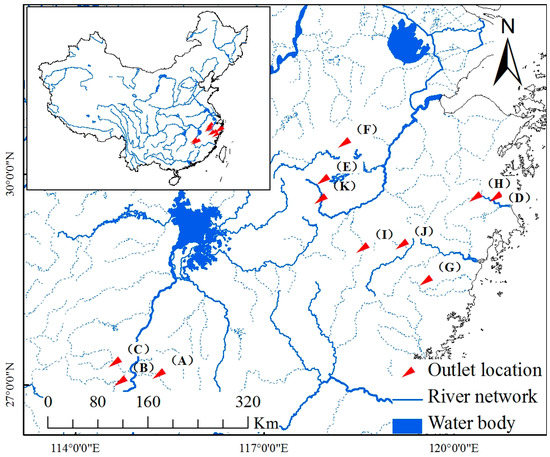
Figure 4.
Location map of the outlet of the studied basins.
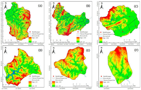
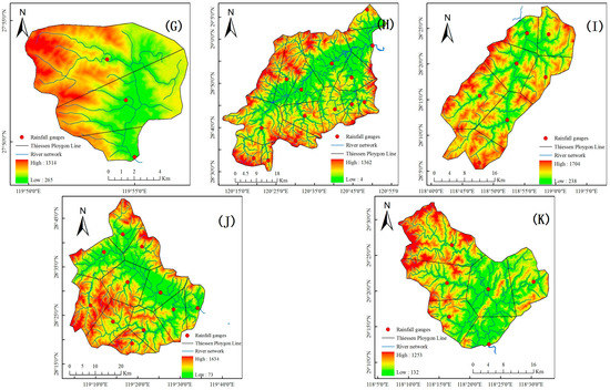
Figure 5.
Location maps of the studied basins. (A) Baisha; (B) Shangshalan; (C) Saitang; (D) Niutoushan Reservoir; (E) Zhongzhou; (F) Yanjia Reservoir; (G) Gaoerdian Reservoir; (H) Bozhiao; (I) Zhonggeng; (J) Jingjukou; (K) Misai.
The main feature of the Xinanjiang model is the concept of runoff generation on repletion of storage, which means runoff is not produced until the soil moisture content of the vadose zone reaches field capacity and thereafter runoff equals the rainfall excess without further loss. The Xinanjiang model consists of three modules: the evapotranspiration module (evapotranspiration of three soil layers), the runoff generating module (runoff production and separation of the runoff into surface runoff, interflow, and ground water), and the flow concentration and river channel routing modules (surface runoff, interflow, and ground water flow concentration and river channel flow routing). The river network flow routing is implemented by lag-and-route method and the river channel flow routing is implemented by Muskingum method. The model has 18 parameters: evapotranspiration parameters including K, UM, LM, WM, and C; runoff production parameters including B and IM; runoff separation parameters including SM, EX, KG, and KI; and flow routing parameters including CG, CI, CS, L, XE, KE and n. The model parameters are determined by manual and PSO-combined optimization method with the flood data shown in the previous sections.
4. Results and Discussion
The Xinanjiang model with and without the ISVC method is used to simulate the flood in each river basin, and the forecasting results, before and after correction of initial state variables, are compared. The following 3 indicators are used to evaluate the effectiveness of the correction [33].
- (1)
- Relative error of flood peak
- (2)
- Relative error of flood total volume
- (3)
- Nash-Sutcliffe coefficient of efficiency
where and represent measured flood peak and calculated flood peak respectively; and represent depth of measured runoff and depth of calculated runoff respectively; is the mean value of measured flow and m is the length of data sequence.
In this paper, the blue histogram represents rainfall, the black solid line represents the measured flow, the red solid line represents the original forecasting flow, the green solid line represents the ISVC corrected forecasting flow, and the red vertical line represents rising time.
4.1. Flood Forecasting without ISVC Method

Table 7.
Calibrated Xinanjiang model parameters of the studied basins.

Table 8.
Each sub-block n of the studied basins.
According to the “Standard for Hydrological Information and Forecasting GB/T 22482-2008” [34], it is qualified when flood forecast errors, including peak flow error and total volume error, do not exceed 20%. Then the qualified rate is obtained by dividing the number of qualified flood events with the total number of flood events. The qualified rate for the 11 basins is shown in Table 9.

Table 9.
Qualified rate of flood forecasting for the 11 studied basins.
Of the 11 basins, the highest qualified rate is in Misai and the lowest is in Baisha with the value of 72.2% and 15.4%, respectively. In addition, the qualified rates of Baizhiao, Zhonggeng, and Jingjukou are also good with the value higher than 65%. In addition, others are lower than 40%, which are in Shangshalan, Saitang, Niutoushan Reservoir, Zhongzhou, Yanjia Reservoir, and Gaoerdian Reservoir.
There are several reasons for the lower qualified rate in some river basins: (1) The density of rainfall stations is insufficient. For example, there are only 8 rainfall stations in Saitang, which means each station controls a very large area of 375 km2 that it cannot reflect the spatial-temporal variability of rainfall; (2) There is no evaporation station in some of the basins such as Baisha, Shangshalan, Zhongzhou, and Yanjia reservoir, which leads to the utilization of the evaporation data nearby that inevitably causes errors; (3) There are some errors in the measured data of the reservoir sections such as Niutoushan Reservoir, Yanjia Reservoir, and Gaoerdian Reservoir. The inflow of the reservoirs is calculated by water balance equation, which means the fluctuation error of reservoir measurement may cause sawtooth phenomenon of the calculated inflow, which affects the flood forecasting results.
4.2. The NRMSE Threshold in Steady Period
Not all forecasts need to be corrected. Given a condition, the floods that satisfies the condition do not need correction, and only the floods that do not meet the condition need to be corrected. Ns is usually used in the flood forecasting to evaluate whether or not the forecasting accuracy is good. However, Ns applies only to sequences that have a non-stable hydrograph, and are often not good for stable hydrographs. For example, the calculated Ns will be positive infinite when the two hydrographs are all with same stable values of q, which is obviously unreasonable. However, the flood process in steady period is usually stable, which means Ns is not suitable to describe error in this scenario. Therefore, an error index (NRMSE) is proposed in this paper to describe the error of steady period. A threshold of NRMSE is required to decide whether the initial state variables need to be corrected. However, the threshold has not been studied in the field of flood forecasting before, that we obtain it by finding the relationship between NRMSE and Ns in this paper.
The Ns and NRMSE of the simulation results for the 360 floods listed in Table 6 are calculated. The two series is sorted by Ns from small to large as shown in Figure 6. The abscissa represents the flood number, the left ordinate represents Ns, and the right ordinate represents NRMSE. It is shown in Figure 6 that with the increasing of Ns, the value of NRMSE decreases. Especially when Ns is closer to 1, NRMSE decreases steadily.
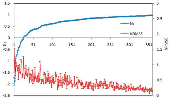
Figure 6.
Comparison between Ns and NRMSE.
It is stipulated in “Standard for Hydrological Information and Hydrological Forecasting GB/T 22482-2008”, when NS > 0.9, the flood forecasting accuracy is recognized as high and therefore no correction is needed. According to the calculation results of 360 flood events, when the value of Ns is between 0.9 and 1, the value of NRMSE is between 0.0593 and 0.4246. The average NRMSE is 0.2212, so the threshold is set to 0.2212. When calculated NRMSE > 0.2212, the initial state variables need correction, otherwise, they do not need to be corrected.
4.3. Overall Performance of the ISVC Method
The ISVC method is used under the threshold constraint to modify the initial state variables of the 360 floods in Table 6, and the results are shown in Table 10. In Table 10, column (2) is the number of flood events that meet the correction criterion of ISVC method; column (3) is the number of flood events with improved accuracy after correction; column (4) is accuracy improvement rate; column (5) is qualified rate before correction; and column (6) is qualified rate after correction.

Table 10.
Correction effect of flood forecasting of each basin.
For the basins with lower qualified rate before correction such as Baisha, Shangshalan, Saitang, Niutoushan Reservoir, Zhongzhou, Yanjia Reservoir, and Gaoerdian Reservoir, the accuracy improvement rate is more than 60% after correction, and the highest is Niutoushan Reservoir with the improvement rate of 78.3%. However, for the basins with higher qualified rate before correction such as Baizhiao, Zhonggeng, Jingjukou, and Misai, the accuracy improvement rate is less than 50% after correction, and the qualified rate reduces after correction. Therefore, the ISVC method is more suitable and effective for basins with lower qualified rate, because when errors in initial state variables are not very high, over-emphasis and over-adjustment on the fitting degree in rising period may cause a lower precision for the whole flood event.
4.4. Comparison of Correction Effectiveness of Different Types of Flood Events
4.4.1. Flood Classification Criteria
The floods are classified into 3 types considering the steady period flood volume forecasting error, the overall flood peak forecasting error and the overall flood volume forecasting error. If all the above-mentioned errors are negative, it is recognized as a under-estimated flood; and if all the above-mentioned errors are positive, it is recognized as an over-estimated flood; and other error scenarios are complex floods. The flood type statistics table of each basin is shown in Table 11.

Table 11.
Flood type statistics of each basin.
In order to demonstrate different flood types, the error statistics of several typical floods are shown in Table 12 and Figure 7, Figure 8 and Figure 9. The figure sequence is consistent with the floods listed in Table 12.

Table 12.
Error statistics of typical floods.
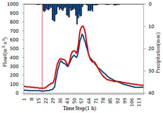
Figure 7.
Under-estimated flood.
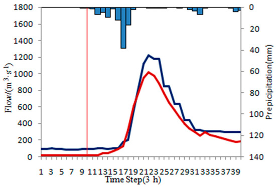
Figure 8.
Over-estimated flood.
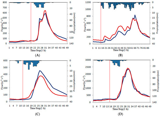
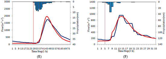
Figure 9.
Complex flood. (A) Zhongzhou; (B) Zhonggeng 17 June 1993 8:00–21 June 1993 0:00; (C) Zhonggeng 22 June 1992 8:00–24 June 1992 8:00; (D) Shangshalan; (E) Jingjukou; (F) Saitang.
4.4.2. Under-Estimated Flood Events
The ISVC method is used to correct the under-estimated floods. Due to the calculated flow is smaller than the measured flow in steady period, the initial state variables should be increased to achieve the purpose of correction. However, there are also some scenarios where the corrected values of the initial state variables are too large, and the accuracy of the whole corrected flood is deteriorated. The correction results of under-estimated floods in each basin is shown in Table 13.

Table 13.
Statistics of correction results of under-estimated floods in each basin.
It is shown in Table 13 the ISVC method performs well for under-estimated floods with 78.8% of floods whose precisions are improved (the fourth columns in Table 13) and 21.2% whose precisions are deteriorated (the sixth columns in Table 13).
To illustrate the results, several typical floods are selected for display. Statistics of typical under-estimated floods are shown in Table 14. The typical hydrographs are shown in Figure 10. The figures sequence is consistent with the floods listed in Table 14.

Table 14.
Statistics of typical under-estimated floods.
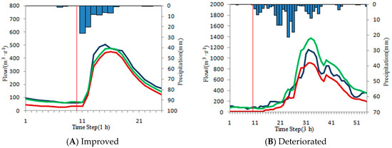
Figure 10.
Accuracy improved and deteriorated floods of under-estimated floods.
4.4.3. Over-Estimated Flood Events
The ISVC method is used to correct the over-estimated floods. Due to the calculated flow is bigger than the measured flow in steady period, the initial state variables should be reduced to achieve the purpose of correction. When the correction degree of the initial state variables is too large, the accuracy of the whole flood correction is deteriorated. The correction results of over-estimated floods in each basin is shown in Table 15.

Table 15.
Statistics of correction results of over-estimated floods in each basin.
It is shown in Table 15 that the ISVC method is also effective for about half of the over-estimated floods with 48.1% of floods whose accuracies are improved and 51.9% whose accuracies are reduced.
To illustrate the results, several typical floods are selected for display. Statistics of typical over-estimated floods are shown in Table 16. The typical hydrographs are shown in Figure 11. The figure sequence is consistent with the floods in Table 16.

Table 16.
Statistics of typical over-estimated floods.
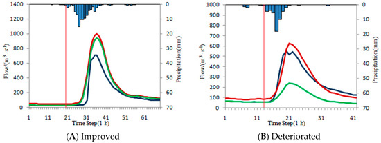
Figure 11.
Accuracy improved and deteriorated floods of over-estimated floods.
4.4.4. Complex Flood Events
As shown in Table 12 and Figure 9, there are 6 types of complex flood events. The correction results of complex floods in each basin are shown in Table 17.

Table 17.
Statistics of correction results of complex floods in each basin.
To illustrate the results, several typical floods are selected for display. Statistics of typical complex floods are shown in Table 18. The typical hydrographs are shown in Figure 12. The figure sequence is consistent with the flood in Table 18.

Table 18.
Statistics of typical complex floods.
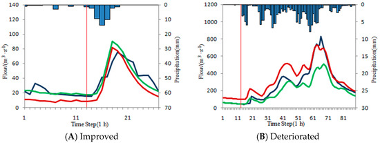
Figure 12.
Accuracy improved and deteriorated floods of complex floods.
4.4.5. Discussions
The ISVC method is applied to 11 basins. The results show that the accuracy-improved rate is up to 78.8% for the under-estimated flood events, while the accuracy-reduced rate is 21.2%. Therefore, the ISVC method has good correction effect on the under-estimated flood events.
The accuracy-improved and the accuracy-reduced rates are 48.1% and 51.9% respectively for the over-estimated flood events. The reason why the accuracy-improved rate is low for the over-estimated flood events is that the qualification rates of the forecast schemes in some basins are already high and further improvements of flood forecasting accuracy by ISVC method is almost impossible. Especially in Baizhiao, Zhonggeng, Jingjukou, and Misai Basins, the qualification rate is already up to 65% and the accuracy-reduced rate is only 43.2% in these four basins. The poor correction results of the above-mentioned four basins deteriorate the total error correction results. Therefore, we must consider the qualification rate of the original prediction scheme before ISVC is carried on. If the qualification rate is already high (such as >60%), we can recognize that the stable period error is reasonable and the correction is not necessary, otherwise the ISVC may cause the over-correction issue, which may lead to the reduction of the flood forecasting accuracy.
The accuracy-improved rate and the accuracy-reduced rate are 22% and 78% respectively for the complex flood. There are two types of complex floods. One is when the positive or negative condition of forecasting error in steady period is contrary to both the overall error of flood volume and the overall error of flood peak. For example, error in steady period is negative, while the overall flood peak error and the overall flood volume is positive and vice versa. This kind of flood is named fully contrary complex flood (FCCF). The study shows that for this type of flood, the ISVC method usually deteriorates the overall flood forecasting result. The other type of complex flood is when the positive or negative condition of forecasting error in steady period is contrary to either the overall error of flood volume or the overall error of flood peak. For example, error in steady period is negative, the overall flood peak error is negative and the overall flood volume error is positive. This kind of flood is named partial contrary complex flood (PCCF). For this type of flood, it is possible to improve the overall flood forecasting result by using the ISVC method.
There are 32 PCCF in the 11 basins with the possibility of improving the accuracy while there are 20 out of 32 floods that are better forecasted after correction. Therefore, the accuracy-improved rate is 20/32 = 62.5%. However, there are 59 FCCF whose accuracy is inevitable reduced after correction that cases the accuracy-improved rate of all the complex floods so low with the value of 22%.
For the floods with lower accuracy after correction, the main reason is that the correction amplitude is too large, which causes the initial state variables to exceed the reasonable ranges. Therefore, the accuracy of the whole flood is reduced after the correction.
Two examples are given to illustrate the accuracy-improved floods and the accuracy-reduced floods after correction.
(1) Flood with better accuracy after correction
Take the flood 1992070315 in Zhongzhou Basin as an example. The flood happened from 3 July 1992 1:00 to 4 July 1992 1:00. The ISVC method is used to modify the initial state variables. The initial state variables are obtained from the daily time-scale Xinanjiang model. The stable period is from 3 July 1992 1:00 to 3 July 1992 9:00. The NRMSE in the stable period is 0.5480, which exceeds the threshold. Deviation U is −38.82, which shows that the error in stable period is large and the forecasted flow is lower than the measured flow. Therefore, the initial state variables need to be corrected. The PSO algorithm is used to modify the coefficient variable (a) of each unit. The ranges of the state variables correction coefficient and the coefficients after optimization are shown in Table 19.

Table 19.
The boundaries and correction results of the state variables coefficients.
Zhongzhou basin is divided into 2 sub-basins. The state variables before and after the optimization are shown in Table 20. Except for QG, other optimized initial state variables reach their corresponding upper boundaries, indicating that the basin is in a very moist state. The default and optimized initial state variables are shown in Table 20.

Table 20.
The initial state variables of the flood 1992070315 in Zhongzhou Basin.
The errors before and after optimization are shown in Table 14 and Figure 10. As shown in Table 14 and Figure 10, the forecasting accuracy is significantly improved by using the ISVC method. The peak error (/%) decreases from −11.11 to −5.75, the volume error (/%) decreases from −19.36 to −6.3, and the Nash-Sutcliffe coefficient increases from 0.9151 to 0.9772, all of which show that the ISVC method is effective for this flood event.
(2) Flood with poor accuracy after correction
Take the flood 1983071303 in Zhonggeng Basin as an example. The flood happened from 12 July 1983 8:00 to 14 July 1983 1:00. The ISVC method is used to modify the initial state variables. The initial state variables are obtained from the daily time-scale Xinanjiang model. The stable period is from 12 July 1983 8:00 to 12 July 1983 20:00. The NRMSE in stable period is 0.4599, which exceeds the threshold. Deviation U is 26.45. Therefore, the initial state variables need to be corrected. The PSO algorithm is used to modify the coefficient variable (a) of each unit. The ranges of the state variables correction coefficient and the coefficients after optimization are shown in Table 21.

Table 21.
The boundaries and correction results of the state variables coefficients.
Zhongzhou basin is divided into 7 sub-basins. The state variables before and after optimization are shown as shown in Table 22. The optimized S is 0, and the QG remains unchanged. The rest of the state variables are smaller than the initial state variables. Therefore, the forecasting flow in stable period after correction is smaller than the initial prediction.

Table 22.
The initial state variables of the flood 1983071303 in Zhonggeng Basin.
The errors before and after optimization are shown in Table 16 and Figure 11. As shown in Table 16 and Figure 11, the forecasting accuracy is significantly decreased after correction. The peak error (/%) increases from 13.32 to −56.88, the volume error (/%) increases from 6.37 to −52.91, and the Nash-Sutcliffe coefficient reduces from 0.9197 to 0.132, all of which shows that the ISVC method is not effective for this flood. Although the forecasting accuracy of the stable period is higher, the forecasting accuracy of the forecasting period is reduced due to the over-correction of the initial state variables. The S changes to 0 by the ISVC method, which may not be consistent with the actual situation, and may be the cause of the larger error after the correction.
The objective function values of the two floods in the process of optimization are shown in Figure 13. In the two optimization processes, both of the objective function values reached a steady state after about 23 iterations. After 44 iterations, the stable condition of the optimization algorithm was reached, and the optimization calculation was stopped, indicating that the efficiency of PSO algorithm is satisfactory.
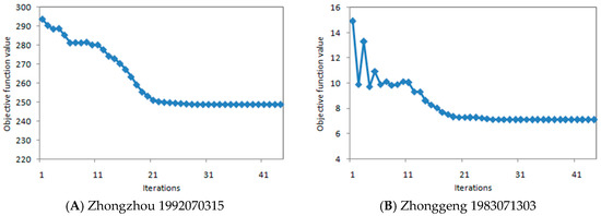
Figure 13.
Objective function values in optimization process.
4.5. Influence of Steady Period Selection
The ISVC method was significantly affected by the steady period selection. In order to demonstrate this problem, we take two flood events in Baizhiao basin as examples.
One flood event happened from 24 August 1983 8:00 to 28 August 1983 8:00. During the flooding period, there is only a little rain from 24 August 1983 8:00 to 25 August 1983 7:00 and the flood peak has not happened considering that the rainfall peak does not arrive (happened at 25 August 1983 16:00). Two rising times are tentatively selected at 25 August 1983 7:00 (Figure 14A) and 25 August 1983 16:00 (Figure 14B). The influence of the rain from 24 August 1983 8:00 to 25 August 1983 7:00 is taken into consideration in the latter rising time. ISVC method is used in the above-mentioned two scenarios and the results are shown in Table 23 and Figure 14. It is found that the correction result is better in the former scenario than the latter one with Ns value being 0.9299 and 0.8469 respectively.
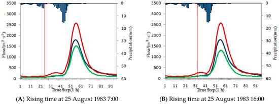
Figure 14.
The flood from 24 August 1983 8:00 to 28 August 1983 8:00 in Baizhiao basin.

Table 23.
Different results of flood correction under different steady periods.
The other flood event in Baizhiao basin happened from 25 July 1987 16:00 to 29 July 1987 12:00. During the flooding period, there is only a little rain from 26 July 1987 21:00 to 27 July 1987 10:00, and the rainfall peak happened at 27 July 1987 12:00. Two rising times are tentatively selected at 26 July 1987 21:00 (Figure 15A) and 27 July 1987 12:00 (Figure 15B). The influence of the rain from 26 July 1987 21:00 to 27 July 1987 12:00 is taken into consideration in the latter scenario. ISVC method is tentatively applied to the two above-mentioned scenarios. In the former scenario, it does not need correction, because the NRMSE of steady period forecast is 0.1848, which is less than the threshold (0.2212). However, in the latter scenario the correction is needed with a larger NRMSE of 0.3489 (larger than 0.2212). The Ns is 0.688 after correction, less than 0.859 before correction. For this flood event, the forecasting result becomes worse after correction. The results are shown in Table 23 and Figure 15.
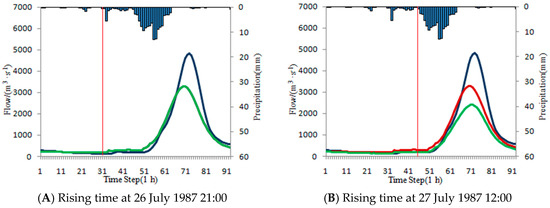
Figure 15.
The flood from 25 July 1987 16:00 to 29 July 1987 12:00 in Baizhiao basin.
The analysis of the above two flood events shows that the selection of the steady period has a significant impact on the application of the ISVC method. The ISVC method is aimed at the correction of the initial state variables, therefore, the smaller the influence of other factors (rainfall, etc.) in the steady period, the better the correction of the initial state variables will be. For selecting the steady period, the impact of the rainfall in steady period should be as little as possible. The rising time should be located at the point when the actual flood and forecasting flood have not risen obviously. At the rinsing time, the rainfall peak is just beginning or the rainfall that causes the flow of the steady period to rise is just ending.
5. Conclusions
A new error correction method for flood forecasting called ISVC is proposed in this paper. In the method, the objective function is established by using the forecasted and measured hydrographs during the steady period and the initial state variables are corrected by the optimization algorithm. After that the corrected initial state variables are used to forecast the flood. The advantages of the ISVC method are as follows:
- (1)
- The ISVC method can be applied before real-time flood forecasting. Only information in steady period is used in the method, while real-time flood forecasting is usually conducted when the rainfall peak has finished. Therefore, unlike other real-time correction methods, the ISVC method can provide accurate initial state variables for real-time flood forecasting;
- (2)
- The ISVC method is applicable to a variety of conceptual hydrological models that have state variables. The ISVC method does not affect structure, parameters, input, and output of flood forecasting models. It does not affect any set of forecasting methods and can be used as a separate module. The ISVC method is suitable for conceptual hydrological models and is easy to popularize and apply;
- (3)
- The ISVC method is simple in principle, convenient in calculation and flexible, and the optimization method can be selected according to the actual situation such as PSO, genetic algorithm, ant colony algorithm, and so on;
- (4)
- Compared with the artificial experience adjustment, the ISVC method is more scientific and standardized, more efficient, and the corrected initial state variables usually obtain higher accuracy and better reliability.
The new method is tested in 11 basins in this paper, and some important issues are also discussed. Several conclusions can be drawn:
- (1)
- The results show that the ISVC method is more effective for the basins with poor qualified rate (less than 60%) of flood forecasting, and the qualified rate can be improved significantly after correction. However, the method is less effective for the basins with high qualified rate (more than 60%) of flood forecasting, and the qualified rate may decrease slightly after correction;
- (2)
- The research on the under-estimated floods, the over-estimated floods and the complex floods shows that ISVC method is suitable for under-estimated floods with 78.8% of floods that have better precision; and the improvement rate of over-estimated floods is 48.1%, which means the ISVC is also effective for half of the over-estimated floods. For the complex floods, it is necessary to predict the future trend of the flood process, predict the specific type of the flood, and then decide whether to use ISVC method.
- (3)
- The selection of the steady period has a direct impact on the correction effectiveness. The study shows that steady period should be before the arrival of the rainfall peak, and the forecasted and measured flow have not risen at the moment.
- (4)
- We should further analyze the sensitivity of each state variable of the Xinanjiang model, study the correlation between the state variables, and further reduce the initial state variables that need to be corrected by the optimization algorithm, so as to reduce the possibility of equifinality of state variables.
Acknowledgments
This research was funded by the National Key Research and Development Program of China (No. 2017YFC0405801, No. 2016YFC0402708); China Postdoctoral Science Foundation on Grant (Grant No. 2016M600096).
Author Contributions
Kuang Li, Liuqian Ding and Guangyuan Kan conceived and designed the experiments; Kuang Li and Kexin Liu performed the experiments; Kuang Li and Guangyuan Kan analyzed the data; Qianjin Dong contributed analysis tools; Lili Liang draw the figures; Kuang Li, Guangyuan Kan; Kexin Liu and Lili Liang wrote the paper.
Conflicts of Interest
The authors declare no conflict of interest.
References
- Bureau of Hydrology, Ministry of Water Resources; Bureau of Hydrology, Changjiang Water Resources Commission. Hand Book of Hydrological Information and Forecast; China Water & Power Press: Beijing, China, 2010.
- Calvo, B.; Savi, F.; Iovine, G. Real-time flood forecasting of the Tiber River in Rome. Nat. Hazards 2009, 50, 461–477. [Google Scholar] [CrossRef]
- Cai, Y.; Jin, C.; Wang, A. Comprehensive precipitation evaluation of TRMM 3B42 with dense rain gauge networks in a mid-latitude basin, Northeast China. Theor. Appl. Climatol. 2016, 126, 659–671. [Google Scholar] [CrossRef]
- Hou, A.; Kakar, R.; Neeck, S. The global precipitation measurement mission. Bull. Am. Meteorol. Soc. 2014, 95, 70l–722. [Google Scholar] [CrossRef]
- Kidd, C.; Huffman, G. Global precipitation measurement. Meteorol. Appl. 2011, 18, 334–353. [Google Scholar] [CrossRef]
- Ministry of Water Resources (MWR). SL34-92 Technical Regulations for Hydrologic Network Design; Water Resources and Electric Power Press: Beijing, China, 1992. (In Chinese)
- Hu, H.; Tian, F. Advancement in research of physically-based watershed hydrological model. J. Hydrol. Eng. 2007, 38, 511–517. (In Chinese) [Google Scholar]
- Nash, J.; Sutcliffe, J. River flow forecasting through conceptual models Part I: A discussion of principles. J. Hydrol. 1970, 10, 282–290. [Google Scholar] [CrossRef]
- Renjun, Z.; Yilin, Z.; Lerun, F. The Xinanjiang model. J. Proc. Oxf. Symp. Hydrol. Forecast. IAHS Publ. 1980, 135, 371–381. [Google Scholar]
- Hu, C.; Guo, S.; Xiong, L.; Peng, D. A Modified Xinanjiang Model and Its Application in Northern China. J. Hydrol. Res. 2005, 36, 175–192. [Google Scholar]
- Wang, W.C.; Cheng, C.T.; Chau, K.W.; Xu, D.M. Calibration of Xinanjiang model parameters using hybrid genetic algorithm-based fuzzy optimal model. J. Hydroinform. 2012, 14, 784–799. [Google Scholar] [CrossRef]
- Yang, S.; Dong, G.; Zheng, D.; Xiao, H.; Gao, Y.; Lang, Y. Coupling Xinanjiang model and SWAT to simulate agricultural non-point source pollution in Songtao watershed of Hainan, China. J. Ecol. Model. 2011, 222, 3701–3717. [Google Scholar] [CrossRef]
- Sugawara, M.; Kite, G.W. The development of hydrological model—Tank. J. Exp. Bot. 1995, 63, 5545–5558. [Google Scholar]
- Zhao, R. Watershed Hydrological Simulation—Xinanjiang Model and Northern Shaanxi Model; Water Resources and Electric Power Press: Beijing, China, 1983. [Google Scholar]
- Rui, X. Discussion of watershed hydrological model. Adv. Sci. Technol. Water Resour. 2017, 37, 1–7. (In Chinese) [Google Scholar]
- Rui, X.; Jiang, C.; Zhang, J. Development of Watershed Hydrologic Models. J. China Hydrol. 2006, 26, 22–26. (In Chinese) [Google Scholar]
- Wang, P.; Zhao, R. Optimazation Method of Calibration of Xinanjiang Model (3 Components). J. Hohai Univ. 1989, 17, 65–69. (In Chinese) [Google Scholar]
- Holland, J.H. Adaptation in Natural and Artificial Systems; University of Michigan Press: Ann Arbor, MI, USA, 1975. [Google Scholar]
- Duan, Q.; GuPta, V.K.; Sorooshian, S. Effective and efficient global Optimization for conceptual rainfall-runoff models. J. Water Resour. Res. 1992, 28, 1015–1031. [Google Scholar] [CrossRef]
- Kennedy, J.; Eberhart, R. Particle Swarm Optimization. In Proceedings of the IEEE Conference on Neural Networks, Perth, Australia, 27 November–1 December 1995; pp. 1942–1948. [Google Scholar]
- Shi, Y.; Eberhart, R.C. A modified particle swarm optimizer. In Proceedings of the IEEE Conference on Evolutionary, Anchorage, AK, USA, 4–9 May 1998; pp. 69–73. [Google Scholar]
- Muste, M.; Yu, K.; Pratt, T.; Abraham, D. Practical aspects of ADCP data use for quantification of mean river flow characteristics; Part II: Fixed-vessel measurement sp. Flow Meas. Instrum. 2004, 15, 17–28. [Google Scholar] [CrossRef]
- Zhu, X.; An, B.; Wang, C. Error Analysis of Real-time Flood Forecasting in Reservoir. J. China Hydrol. 1997, 6, 20–24. (In Chinese) [Google Scholar]
- Weerts, A.H.; El Serafy, G.Y.H. Particle Filtering and Ensemble Kalman Filtering for state updating with hydrological conceptual rainfall runoff models. J. Water Resour. Res. 2006, 42, 123–154. [Google Scholar] [CrossRef]
- Komma, J.; Reszler, C.; Blöschl, G. Soil moisture updating by Ensemble Kalman Filtering in real-time flood forecasting. J. Hydrol. 2008, 357, 228–242. [Google Scholar] [CrossRef]
- Li, Z.; Xin, P.; Tang, J. Study of the Xinanjiang Model Parameter Calibration. J. Hydrol. Eng. 2011, 18, 1513–1521. [Google Scholar]
- Zhuo, L.; Han, D. Misrepresentation and amendment of soil moisture in conceptual hydrological modelling. J. Hydrol. 2016, 535, 637–651. [Google Scholar] [CrossRef]
- Liu, J.; Zhang, J. Effect of antecedent Soil Water Content on the Uncertainty of Hydrological Simulation. J. Glaciol. Geocryol. 2006, 28, 519–525. [Google Scholar]
- Wu, X.; Xiang, X.; Wang, C. Coupled Hydraulic and Kalman Filter Model for Real-Time Correction of Flood Forecast in the Three Gorges Interzone of Yangtze River, China. J. Hydrol. Eng. 2013, 18, 1416–1425. [Google Scholar] [CrossRef]
- Jian, X.; Zheng, J. Analysis of algorithms and error evaluation criteria in chaotic neural network predictions. J. Tsinghua Univ. 2001, 41, 43–46. (In Chinese) [Google Scholar]
- Kan, G.; He, X.; Li, J.; Ding, L.; Hong, Y.; Zhang, H.; Liang, K.; Zhang, M. Computer Aided Numerical Methods for Hydrological Model Calibration: An Overview and Recent Development. Arch. Comput. Methods Eng. 2017, 25, 1–25. [Google Scholar] [CrossRef]
- Kan, G.; Lei, T.; Liang, K.; Li, J.; Ding, L.; He, X.; Yu, H.; Zhang, D.; Zuo, D.; Bao, Z.; et al. A multi-core CPU and many-core GPU-based fast parallel shuffled complex evolution global optimization approach. IEEE Trans. Parallel Distrib. Syst. 2017, 28, 332–344. [Google Scholar] [CrossRef]
- Bao, W.; Que, J.; Lai, S.; Wei, S. Free-water storage error correction based on dynamic system response in flood forecasting. Adv. Water Sci. 2015, 26, 365–371. (In Chinese) [Google Scholar]
- Ministry of Water Resources (MWR). 2008 Standard for Hydrological Information and Hydrological Forecasting; GB/T 22482; Water Resources and Electric Power Press: Beijing, China, 2008. (In Chinese)
© 2017 by the authors. Licensee MDPI, Basel, Switzerland. This article is an open access article distributed under the terms and conditions of the Creative Commons Attribution (CC BY) license (http://creativecommons.org/licenses/by/4.0/).