Abstract
This study analyzed all characteristics of the error committed in evaluating annual maximum rainfall depth, Hd, associated with a given duration, d, when data with coarse temporal aggregation, ta, were used. It is well known that when ta = 1 min, this error is practically negligible while coarser temporal aggregations can determine underestimation for a single Hd up to 50% and for the average value of sufficiently numerous series of Hd up to 16.67%. By using a mathematical relation between average underestimation error and the ratio ta/d, each Hd value belonging to a specific series could be corrected through deterministic or stochastic approaches. With a deterministic approach, an average correction was identically applied to all Hd values with the same ta and d while, for a stochastic correction, a thorough knowledge of the statistical characteristics of the underestimation error was required. Accordingly, in this work, rainfall data derived from many stations in central Italy were analyzed and it was assessed that single and average errors, which were both assumed as random variables, followed exponential and normal distributions, respectively. Furthermore, the single underestimation error was also found inversely correlated to the corresponding annual maximum rainfall depth.
1. Introduction
Precipitation knowledge is essential for many hydrologic studies and applications including studies on rainfall modeling [1,2,3], interception losses [4], infiltration modeling [5,6,7], runoff generation [8,9,10,11,12,13], soil erosion [14], floods [15,16,17], and droughts [18,19].
Rainfall data may be available with temporal aggregation (or time resolution), ta, that varies depending on the technologies used (for example, a recording system with paper rolls, which was largely adopted in the past, allowed hourly or half hourly aggregations) and the procedures followed by the rain gauge station manager. Nowadays, through the use of tipping bucket sensors, all tipping times are recorded in a digital data-logger with each tip equal to a well-known depth (typically 0.1 mm or 0.2 mm). Then, the rainfall characteristics such as rain rates are obtained by aggregating the number of tips over selected ta, which is a variable between one minute and 24 h.
When rainfall data are aggregated, their analyses at a time scale smaller than the adopted ta are not possible. In addition, the specific choice regarding ta could also influence the results of the analyses involving time durations greater than or equal to ta itself [20].
It is well known that rainfall data recorded at fixed temporal aggregations may underestimate true maximum accumulations for durations, d, equal or comparable with ta [21,22,23,24,25]. Reference [21] observed that multiplying the results of a frequency analysis of Hd by 1.13 yields values very close to those derived from analyses based on true maxima [22] by assuming that a uniform rainfall occurring over the duration of interest developed a theoretical relationship between the sampling adjustment factor (SAF) versus ta/d where SAF is the average ratio of the true maximum accumulation to the maximum given by a fixed interval gauge record [23] by using high temporal resolution data, which found a relationship between SAF and ta/d more consistent with other empirical studies [26,27,28]. However, the analyzed series length within the range of 5.3 years to 14.9 years was too limited to perform results of general validity [24] following the [21] theoretical approach. This found that a correction factor (CF), which was a parameter with the same practical meaning of the SAF adopted by Reference [23], depends on the rainfall temporal distribution. More recently, reference [25] defined a procedure to derive quasi-homogeneous Hd series starting from inhomogeneous series with a percentage of values obtained from coarse rainfall data (typically old data) and another percentage derived from continuous data (recorded in the last 20 to 30 years). In detail, for each d value, a mathematical relation between average underestimation error, Ea%, and the ratio ta/d can be used to correct the Hd values. This correction can be carried out with different approaches of deterministic or stochastic types.
Through a deterministic approach, an average correction is identically applied to all Hd values characterized by the same ta and d while, for a more realistic correction, a stochastic approach, which requires a thorough knowledge of the statistical characteristics of the underestimation error, should be used. In the last case, each underestimated Hd value is modified/corrected by using a specific value of the single underestimated error, E%, treated as a random variable.
Among the most important determinations that may take place with precipitation data, there are the rainfall depth-duration-frequency relationships [29,30,31,32], which can be determined by starting from the annual maximum rainfall depths, Hd, cumulated over different durations, d [33]. The use of uncorrected Hd series determines rainfall depth-duration frequency curves with underestimation in the interval of 5% to 10% depending on the return period and duration [25]. Furthermore, the underestimation of Hd values due to coarse ta plays a significant role in the analysis of the effect of climatic change on extreme rainfall. In fact, the correction of the values can vary the sign of the trend from positive to negative especially for series where the probability of the presence of values with ta/d = 1 is particularly high [34].
On this basis, the main objective of this paper is to analyze the behavior of the probability distribution function for both single and average underestimation error variables. The second task of this study is to define, if existing, the correlation law between the single underestimation error and the corresponding annual maximum rainfall depth.
2. Case Study
Rainfall information used in this study were observed in a geographical area of central Italy known as the Umbria region (8456 km2). This area has a very complex orography along the East boundary where the Apennine Mountains exceed 2000 m a.s.l. while it is mainly hilly in the central and western areas with elevation in the interval 100 m a.s.l. to 800 m a.s.l.
The mean annual rainfall is about 900 mm, which ranged over the region from 650 mm to 1450 mm (on the basis of the observation period 1921–2015 and a network of 93 rain gauges). Higher monthly rainfall values generally occur during the autumn-winter period with floods caused by widespread rainfalls. Mean annual air temperature ranges on a monthly base from 3.3 °C to 14.2 °C with maximum values during the month of July and minimum values during January.
A wide percentage of the study area is included in the Tiber River basin. In fact, the Tiber River crosses the region from the North to the South-West receiving water from many tributaries, which is mainly located on the hydrographic left side.
The Umbria region is presently monitored through a network characterized by one rain gauge for each 90 km2 with all devices continuously connected to a central unit through a radio link while, before 1992, only 18 rain gauges with measurements made every 30 min were installed.
In this study, 16 rain gauge stations characterized by the best quality of continuous rainfall data recorded for at least 20 years are considered. Their geographic position and main characteristics are reported in Figure 1 and Table 1.
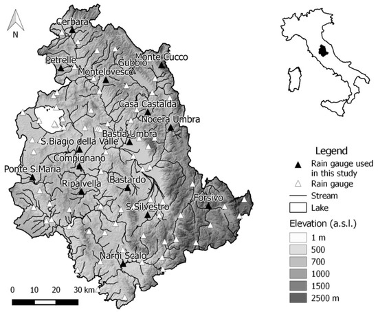
Figure 1.
Morphology and the rain gauge network of the Umbria region. The position of the rain gauges used in the analysis is also shown.

Table 1.
Main characteristics of the selected rainfall stations located in the Umbria region (central Italy). The geographic location is in Universal Transvers Mercator (UTM) coordinates computing by using the WGS84 ellipsoid model.
3. Methods
The accumulated rainfall recorded over a time interval d, xd can be obtained through the following procedure [35,36].
where x(t) is the rainfall rate at time t.
Then the annual maximum rainfall depth over a duration d, Hd, may be easily derived through the following equation.
with t0 equal to the initial instant of the year.
To obtain Hd for each year, the knowledge of rainfall data with any ta ≤ d is request. Since it can be seen in Figure 2, the Hd value is sometimes correctly estimated (Figure 2a) while sometimes it is underestimated (Figure 2b,c) with single errors that may reach the 50% (Figure 2c).
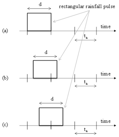
Figure 2.
Representation of a generic rainfall pulse characterized by duration, d, equal to the measurement temporal resolution, ta. (a) Case where a correct determination of the annual maximum rainfall depth of duration d, Hd, is possible. (b) Case with a generic underestimation of Hd. (c) Case with the maximum underestimation of Hd (50%).
For every duration d, a very long Hd series is affected by underestimations depending on both ta and the shape of the rainfall pulses [25]. If we consider pulses with a rectangular shape, when ta = d, the average error, Ea%, is equal to 25% because all errors assume an equal probability of occurrence values between 0% and 50% while, in the case of triangular pulses, the average underestimation becomes 16.67%. However, an analysis of a large number of rainfall events observed in different stations and d values highlights that, before and after the peak, the rainfall depth exhibits a steeper trend. For instance, Figure 3 shows three rainfall events associated with the Hd for d = 60 min that were observed in a station of central Italy. Therefore, the actual value of Ea% should be less than the theoretical value of 16.67% [24].
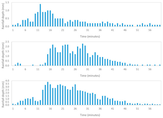
Figure 3.
Sample hyetographs recorded at the Bastardo station (Umbria Region, central Italy) involving annual maximum rainfall depths for d = 60 min. From top to bottom, moving windows selected for the years 1993, 1998, and 2011.
We note that, in principle, underestimation errors in determining the Hd values cannot be eliminated independently of the adopted ta. However, if d = ta = 1 min for an extreme rainfall event of intensity equal to 300 mm/h, the underestimation error becomes negligible. Furthermore, considering that the durations of interest for Hd are typically ≥5 min, observed rainfall characterized by ta = 1 min may be assumed as continuous data characterized by a negligible error. In any case, the largest average error occurs for ta = d and decreases when the ratio ta/d decreases.
Considering rainfall data with temporal aggregations in the interval of 1 to 1440 min, the methodology adopted in this study mainly consists of the analysis of a large number of underestimation errors obtained during the evaluation of annual maximum rainfall depths with durations between 10 min to 2880 min.
Starting from the rainfall measurements (tipping times) for each selected station, aggregated data with the following ta were obtained: 1 min, henceforth denoted as “Observed”; 10 min, 15 min, 30 min, 60 min, 180 min, 360 min, 720 min and 1440 min, henceforth all denoted as “Generated”. This procedure is clearly explained in Table 2 for a reduced set of rainfall data observed at the Gubbio rain gauge. As it can be seen, the first column on the left represents measured rainfall depths with temporal aggregation equal to 1 min. The other columns (“Generated” rainfall depth) can be derived from the first through easy addition operations. For example, the top rainfall depth with ta = 10 min, equal to 1.6 mm, is the sum of the top 10 observed values (0.2, 0.2, 0.0, 0.2, 0.2, 0.4, 0.0, 0.2, 0.2, 0.0).
Table 2.
“Observed” and “Generated” rainfall data characterized by different time resolutions, ta, starting from 3 January 2017 at 6:00 a.m. at the Gubbio rain gauge, located in the Umbria Region.
For all selected stations and considering some typical durations (≤1440 min), all annual maximum rainfall depths may be determined by using both the “Observed” and “Generated” data. Obviously, for each set of rainfall data, Hd can be evaluated only for d ≥ ta.
Considering all Hd values derived from the “Observed” rainfall data as a benchmark, the annual maximum rainfall depth errors due to the use of rainfall data with a coarse ta (“Generated”) can be determined. For example, Table 3 and Table 4 emphasize the single underestimation errors for Nocera Umbra rain gauge considering ta values equal to 30 and 15 min, respectively. As it can be seen, for fixed ta and d, underestimations can randomly vary with years. In Table 3, for ta = d = 30 min, the minimum underestimation error is practically negligible (0.01% in 2009) while it increases to 48.74% in 2010. It may be deduced that significant underestimations occur when ta is equal to d, whereas they become negligible when ta/d ≤ 0.1.
Table 3.
Single underestimation errors, E%, (in%) in the determination of the annual maximum rainfall depth considering rainfall data with temporal resolution equal to 30 min and various durations, d, at the Nocera Umbra rain gauge, located in the Umbria Region. For each d, the average underestimation error, Ea%, is also reported.
Table 4.
Single underestimation errors, E%, (in %) in the determination of the annual maximum rainfall depth considering rainfall data with temporal resolution equal to 15 min and various durations, d, at the Nocera Umbra rain gauge, located in the Umbria Region. For each d, the average underestimation error, Ea%, is also reported.
4. Results and Discussion
4.1. Single Error Analysis
With the main purpose to determine the best probability function representing the single underestimation error assumed as a random variable, all errors on the annual maximum rainfall depth due to the use of “generated” data characterized by temporal aggregation in the range of 10 to 1440 min were first grouped considering different ta/d ratios. Then, dividing the well-known range of possible individual errors (0–50%) into a reasonable number of classes, for each ta/d, the relative frequency of underestimation errors has been determined. As an example, Figure 4 shows the histograms of the relative frequency for three representative cases. Figure 4c points out that, for low values of the ta/d ratio, an adequate representation of the errors’ frequency is possible only if a reduced amplitude of the classes is considered (see Figure 5).
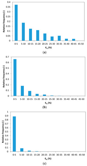
Figure 4.
Relative frequency of the underestimation error, E%, of the maximum rainfall depths considering classes amplitude equal to 5%. (a) ta/d = 1. (b) ta/d = 0.5. (c) ta/d = 0.333. All selected rain gauge stations and all possible combinations of ta and d were considered.
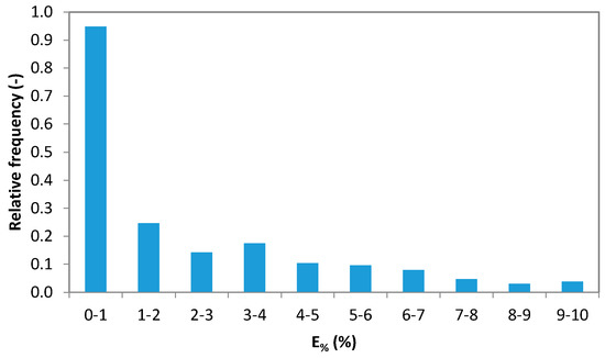
Figure 5.
Similar to Figure 4c but with classes’ amplitude equal to 1%.
Since a specific ta/d ratio may result from different ta values, it has been verified whether this dependence produces any significant effect on the relative frequency histograms. Figure 6 shows the behavior of three histograms for cases with the same ta/d (equal to 1) but with different ta (equal to 30 min, 60 min, and 1440 min).
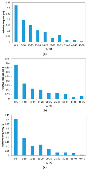
Figure 6.
Relative frequency of the underestimation error, E%, of the maximum rainfall depths considering classes’ amplitude equal to 5%. (a) ta = d = 30 min, (b) ta = d = 60 min, and (c) ta = d = 1440 min. All selected rain gauge stations were considered.
Based on the analysis of Figure 4, Figure 5 and Figure 6, the shape of the histograms seems to be the same independently of ta and d. The best mathematical equation representing these trends was the exponential curve according to the most common statistical tests (Pearson, Kolmogorov-Smirnov, and Anderson-Darling). It is characterized by the following probability density and cumulative distribution functions, respectively.
where the parameter λ (>0) is the inverse of the sample expected value.
On this basis, the characterization of the single underestimation error only depends on the parameter λ. Considering all rainfall data observed in the selected stations and all possible combinations of ta and d, Figure 7 displays λ values as a function of the ta/d ratios. The best interpolation function can be expressed by the equation below.
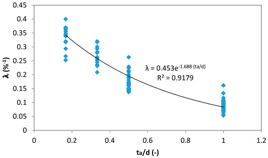
Figure 7.
Behavior of the λ parameter as a function of the ratio between temporal aggregation, ta, and duration, d, for all selected rainfall stations and for ta/d ≥ 0.1666. The best interpolating function is also plotted.
However, from our results, we observed that the assessment of λ could be further improved by splitting Equation (5) on the basis of the d value because of its link with the shape of the rainfall hyetograph that influences the error magnitude [24]. Rectangular hyetographs were typically observed for d up to 30 min, triangular hyetographs for greater values of d up to 180 min, and pulses represented by quadratic functions [24] for larger values of d. As a consequence, the following three relations, which are plotted in Figure 8, were derived.
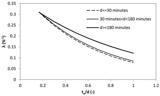
Figure 8.
Behavior of the λ parameter obtained by Equations (6)–(8) depending on ratio ta/d where ta is the time resolution of rainfall data and d is the duration.
For each ratio ta/d and for each d value, Equations (6)–(8) can be used to obtain the parameter λ to be applied when the generation of E% values is necessary.
4.2. Average Error Analysis
The main characteristics of the average underestimation error of annual maximum rainfall depth, Ea%, were analyzed by Reference [25]. They concluded that, in the worst conditions that occur for ta = d, the Ea% for a series of appropriate length is less than or equal to 16.67% and developed reliable relationships between Ea% and values of ta and d. In this work, as an element of novelty, the analysis of the statistical distribution of the average error was carried out.
Additionally, for the average underestimation error, the relative frequency was evaluated by considering different ta/d ratios and adequate classes’ amplitudes. From the visual analysis of Figure 9 and, from the adoption of the main statistical tests (Pearson, Kolmogorov-Smirnov, Anderson-Darling), it may be deduced that the following normal distribution function correctly represents the behavior of the random variable.
where μ and σ are the sample expected value and standard deviation, respectively.
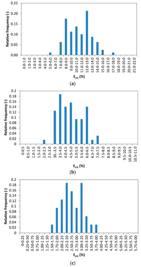
Figure 9.
Relative frequency of the average underestimation error, Ea%, of the maximum rainfall depth, which considers the classes’ amplitudes shown in the x-axis. (a) ta/d = 1, (b) ta/d = 0.5, and (c) ta/d = 0.333. All selected rain gauge stations and all possible combinations of ta and d were considered.
For the μ parameter, results relevant to Morbidelli et al. (2017) were obtained. In fact, in this case, the results showed that the μ parameter depends on both the ta/d ratio and d. Specifically, for ta/d = 1 values of μ = 12.40%, 11.89%, and 10.41% were found for d = 30 min, 60 min, and 1440 min, respectively. The characteristic behavior of the σ parameter is shown in Table 5. At increasing values of μ, corresponding values of σ and cv = σ/μ increase and decrease, respectively. This last trend shows that the dispersion of the values of the random variable increases in conditions of reduced values of μ and decreases in the cases of greater practical interest.
Table 5.
Observed behavior of the parameters μ, σ, and cv (=σ/μ) of Equation (9) as a function of the ratio ta/d where ta is the time resolution of rainfall data and d is the duration.
4.3. Correlation Hd-Error
The analysis of the underestimation error of the annual maximum rainfall depths is very important when systematic corrections on Hd series affected by this problem have to be carried out. In this context, it is necessary to analyze the possible link between each single underestimation error with the corresponding Hd. To this aim, all possible combinations of ta and d were analyzed. In 78% of cases, a negative correlation between the considered quantities was found. In Figure 10, an example of this type of result for three different cases is shown. Note that while in most cases, an inverse link between the underestimation error and the annual maximum rainfall depth was highlighted, the probability of incurring an opposite result is not negligible (22%). However, in almost all cases with a direct correlation between the single error and Hd, the magnitude of the link was very limited, which was shown in Figure 11.
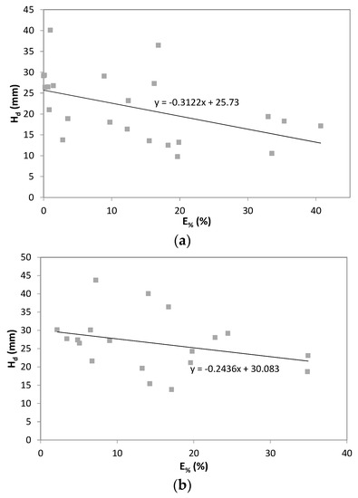
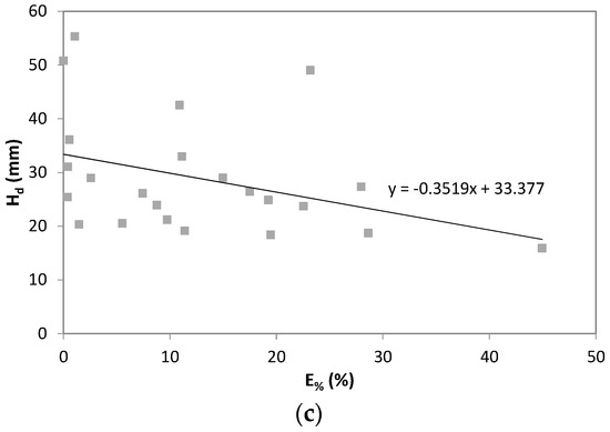
Figure 10.
Relation between the annual maximum rainfall depth, Hd, and the underestimation error, E%. (a) Cerbara station, ta = d = 30 min. (b) Montecucco station, ta = d = 60 min. (c) Casa Castalda station, ta = d = 60 min. The best interpolating linear function is also plotted.
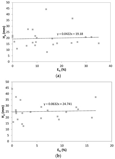
Figure 11.
Relation between annual maximum rainfall depth, Hd, and underestimation error, E%. (a) San Biagio della Valle station, ta = d = 30 min. (b) Compignano station, ta = 15 min and d = 30 min. The best interpolating linear function is also plotted.
4.4. Correction Procedure
When a series of n annual maximum rainfall depths, (i = 1, …, n), of assigned duration d obtained from data characterized by coarse ta has to be corrected, the steps below are followed.
- The λ parameter of the exponential distribution function (Equation (3) or Equation (4)) through the use of Equations (6)–(8) has to be quantified.
- A set of underestimation errors (i = 1, …, n), respecting the probability density function of point 1, has to be generated,
- Each generated value has to be combined with a specific uncorrected on the basis of the inverse correlation between these quantities.
- Each has to be corrected in accordance with the following equation.where and are the corrected and uncorrected values, respectively.
- In the case of the Montecarlo procedure, steps 2, 3, and 4 have to be repeated.
5. Conclusions
On the basis of analyses and results reported in this study, the following conclusions are drawn.
- -
- Annual maximum rainfall depth series derived from very old data inevitably involve many underestimated values due to the adoption of recording systems that only recently allow very small temporal aggregations.
- -
- The underestimated Hd values due to the coarse temporal aggregation of historical rainfall data may be minimized/eliminated through the use of deterministic or stochastic approaches.
- -
- In the deterministic approach, an average correction is identically applied to all Hd values characterized by the same ta and d.
- -
- In the stochastic approach, a more complex procedure can be adopted, which requires a thorough knowledge of the statistical characteristics of the underestimation error.
- -
- The single underestimation error follows an exponential distribution law characterized by a parameter linked to ta and d.
- -
- The average underestimation error follows a normal distribution law characterized by two parameters, which include the expected value and the standard deviation. This produces a reduced dispersion of the random variable in cases of greater practical interest.
- -
- The correlation between the single underestimation error and the corresponding maximum annual rainfall depth can be assumed inversely related with a probability of 78%.
By using the results of this paper, each Hd series containing underestimated values may be easily corrected/modified and become quasi-homogeneous by adopting a stochastic approach. In fact, starting from the knowledge of the ta and d values, all necessary characteristics of the statistical distribution laws representing the underestimated error could be derived. All generated errors can also be associated with the uncorrected Hd values respecting the verified link between them, which is predominantly of the inverse type.
Note that the results of this paper have been derived by using rainfall data observed in central Italy and should be valid in each geographical area of the world characterized by similar environmental conditions.
Author Contributions
Data curation, R.M., C.S., A.F., T.P., J.D., and C.C. Formal analysis, C.C. Methodology, R.M., C.S., A.F., T.P., J.D., and C.C. Supervision, R.M., C.S., A.F., and C.C. Writing—original draft, R.M., C.S., A.F., T.P., J.D., and C.C. Writing—review & editing, R.M., C.S., A.F., T.P., J.D., and C.C.
Funding
This research received no external funding.
Acknowledgments
The authors wish to thank the Functional Center of the Umbria Region for providing all the rainfall information and E. Pauselli and M. Stelluti for their technical assistance.
Conflicts of Interest
The authors declare no conflict of interest.
References
- Woolhiser, D.A.; Osborn, H.B. A stochastic model of dimensionless thunderstorm rainfall. Water Resour. Res. 1985, 21, 511–522. [Google Scholar] [CrossRef]
- Abdo, K.S.; Fiseha, B.M.; Rientjes, T.H.M.; Gieske, A.S.M.; Haile, A.T. Assessment of climate change impacts on the hydrology of Gilgel Abay catchment in Lake Tana basin, Ethiopia. Hydrol. Process. 2009, 23, 3661–3669. [Google Scholar] [CrossRef]
- Haile, A.T.; Rientjes, T.H.M.; Gieske, A.; Jetten, V.; Mekonnen, G. Satellite remote sensing and conceptual cloud modelling for convective rainfall simulation. Adv. Water Resour. 2011, 34, 26–37. [Google Scholar] [CrossRef]
- Zeng, N.; Shuttleworth, J.W.; Gash, J.H.C. Influence of temporal variability of rainfall on interception loss, Part I. Point analysis. J. Hydrol. 2000, 228, 228–241. [Google Scholar] [CrossRef]
- Melone, F.; Corradini, C.; Morbidelli, R.; Saltalippi, C.; Flammini, A. Comparison of theoretical and experimental soil moisture profiles under complex rainfall patterns. J. Hydrol. Eng. 2008, 13, 1170–1176. [Google Scholar] [CrossRef]
- Morbidelli, R.; Corradini, C.; Saltalippi, C.; Flammini, A.; Rossi, E. Infiltration-soil moisture redistribution under natural conditions: Experimental evidence as a guideline for realizing simulation models. Hydrol. Earth Syst. Sci. 2011, 15, 2937–2945. [Google Scholar] [CrossRef]
- Morbidelli, R.; Saltalippi, C.; Flammini, A.; Rossi, E.; Corradini, C. Soil water content vertical profiles under natural conditions: Matching of experiments and simulations by a conceptual model. Hydrol. Proc. 2014, 28, 4732–4742. [Google Scholar] [CrossRef]
- Milly, P.; Eagleson, P. Effect of storm scale on surface runoff volume. Water Resour. Res. 1988, 24, 620–624. [Google Scholar] [CrossRef]
- Govindaraju, R.S.; Morbidelli, R.; Corradini, C. Use of similarity profiles for computing surface runoff over small watersheds. J. Hydrol. Eng. 1999, 4, 100–107. [Google Scholar] [CrossRef]
- Zhang, G.P.; Fenicia, F.; Rientjes, T.H.M.; Reggiani, P.; Savenije, H.H.G. Modeling runoff generation in Geer river basin with improved model parameterization to the REW approach. Phys. Chem. Earth 2005, 30, 285–296. [Google Scholar] [CrossRef]
- Kusumastuti, D.I.; Struthers, I.; Sivapalan, M.; Reynolds, D.A. Threshold effects in catchment storm response and the occurrence and magnitude of flood events: Implications for flood frequency. Hydrol. Earth Syst. Sci. 2007, 11, 1515–1528. [Google Scholar] [CrossRef]
- De Vos, N.J.; Rientjes, T.H.M. Multi-objective training of artificial neural networks for rainfall-runoff modelling. Water Resour. Res. 2008, 44. [Google Scholar] [CrossRef]
- Morbidelli, R.; Saltalippi, C.; Flammini, A.; Corradini, C.; Brocca, L.; Govindaraju, R.S. An investigation of the effects of spatial heterogeneity of initial soil moisture content on surface runoff simulation at a small watershed scale. J. Hydrol. 2016, 539, 589–598. [Google Scholar] [CrossRef]
- Angel, J.R.; Palecki, M.A.; Hollinger, S.E. Storm precipitation in the United States, Part II: Soil erosion characteristics. J. Appl. Meteorol. 2005, 44, 947–959. [Google Scholar] [CrossRef]
- Camici, S.; Tarpanelli, A.; Brocca, L.; Melone, F.; Moramarco, T. Design soil moisture estimation by comparing continuous and storm-based rainfall-runoff modeling. Water Resour. Res. 2011, 47. [Google Scholar] [CrossRef]
- Faccini, F.; Paliaga, G.; Piana, P.; Sacchini, A.; Watkins, C. The Bisagno stream catchment (Genoa, Italy) and its major floods: Geomorphic and land use variations in the last three centuries. Geomorphology 2016, 273, 14–27. [Google Scholar] [CrossRef]
- Vormoor, K.; Lawrence, D.; Schlichting, L.; Wilson, D.; Wong, W.K. Evidence for changes in the magnitude and frequency of observed rainfall vs. snowmelt driven floods in Norway. J. Hydrol. 2016, 538, 33–48. [Google Scholar] [CrossRef]
- Masud, M.B.; Khaliq, M.N.; Wheater, H.S. Analysis of meteorological droughts for the Saskatchewan River Basin using univariate and bivariate approaches. J. Hydrol. 2015, 522, 452–466. [Google Scholar] [CrossRef]
- Mallya, G.; Mishra, V.; Niyogi, D.; Tripathi, S.; Govindaraju, R.S. Trends and variability of droughts over the Indian monsoon region. Weather Clim. Extr. 2016, 12, 43–68. [Google Scholar] [CrossRef]
- Haile, A.T.; Rientjes, T.H.M.; Habib, E.; Jetten, V.; Gebremichael, M. Rain event properties at the source of the Blue Nile River. Hydrol. Earth Syst. Sci. 2011, 15, 1023–1034. [Google Scholar] [CrossRef]
- Hershfield, D.M. Rainfall Frequency Atlas of the United States for Durations From 30 Minutes to 24 Hours and Return Periods from 1 to 100 Years; US Weather Bureau Technical Paper N. 40; U.S. Dept. of Commerce: Washington, DC, USA, 1961. Available online: https://www.lm.doe.gov/cercla/documents/fernald_docs/CAT/109669.pdf (accessed on 1 August 2018).
- Weiss, L.L. Ratio of true to fixed-interval maximum rainfall. J. Hydraul. Div. 1964, 90, 77–82. [Google Scholar]
- Young, C.B.; McEnroe, B.M. Sampling adjustment factors for rainfall recorded at fixed time intervals. J. Hydrol. Eng. 2003, 8, 294–296. [Google Scholar] [CrossRef]
- Yoo, C.; Jun, C.; Park, C. Effect of rainfall temporal distribution on the conversion factor to convert the fixed-interval into true-interval rainfall. J. Hydrol. Eng. 2015, 20. [Google Scholar] [CrossRef]
- Morbidelli, R.; Saltalippi, C.; Flammini, A.; Cifrodelli, M.; Picciafuoco, T.; Corradini, C.; Casas-Castillo, M.C.; Fowler, H.J.; Wilkinson, S.M. Effect of temporal aggregation on the estimate of annual maximum rainfall depths for the design of hydraulic infrastructure systems. J. Hydrol. 2017, 554, 710–720. [Google Scholar] [CrossRef]
- Miller, J.F.; Frederick, R.H.; Tracey, R.J. Precipitation-frequency atlas of the western United States. In NOAA Atlas 2; National Weather Service, National Oceanic and Atmospheric Administration, U.S. Dept. of Commerce: Washington, DC, USA, 1973. Available online: https://repository.library.noaa.gov/view/noaa/7303 (accessed on 1 August 2018).
- Frederick, R.H.; Myers, V.A.; Auciello, E.P. Five-to 60-min Precipitation Frequency for the Eastern and Central United States; NOAA Technical Memorandum NWS HYDRO-35; National Oceanic and Atmospheric Administration, National Weather Service: Silver Spring, MD, USA, 1977. Available online: https://repository.library.noaa.gov/view/noaa/6435 (accessed on 1 August 2018).
- Huff, F.A.; Angel, J.R. Rainfall Frequency Atlas of the Midwest. In Illinois State Water Survey Bulletin 71, Midwest Climate Center Research Rep. 92-03; Illinois State Water Survey: Champaign, IL, USA, 1992; Available online: https://www.ideals.illinois.edu/bitstream/handle/2142/94532/ISWSB-71.pdf?sequence=1 (accessed on 1 August 2018).
- Sivapalan, M.; Bloschl, G. Transformation of point rainfall to areal rainfall: Intensity-duration-frequency curves. J. Hydrol. 1998, 204, 150–167. [Google Scholar] [CrossRef]
- Willems, P. Compound intensity/duration/frequency-relationships of extreme precipitation for two seasons and two storm types. J. Hydrol. 2000, 233, 189–205. [Google Scholar] [CrossRef]
- Overeem, A.; Buishand, A.; Holleman, I. Rainfall depth-duration-frequency curves and their uncertainties. J. Hydrol. 2008, 348, 124–134. [Google Scholar] [CrossRef]
- De Michele, C.; Zenoni, E.; Pecora, S.; Rosso, R. Analytical derivation of rain intensity-duration-area-frequency relationships from event maxima. J. Hydrol. 2011, 399, 385–393. [Google Scholar] [CrossRef]
- Koutsoyiannis, D.; Kozonis, D.; Manetas, A. A mathematical framework for studying rainfall intensity-duration-frequency relationships. J. Hydrol. 1998, 206, 118–135. [Google Scholar] [CrossRef]
- Morbidelli, R.; Saltalippi, C.; Flammini, A.; Corradini, C.; Wilkinson, S.M.; Fowler, H.J. Influence of temporal data aggregation on trend estimation for intense rainfall. Adv. Water Resour. 2018, in press. [Google Scholar]
- Burlando, P.; Rosso, R. Scaling and multiscaling models of depth-duration-frequency curves for storm precipitation. J. Hydrol. 1996, 187, 45–64. [Google Scholar] [CrossRef]
- Boni, G.; Parodi, A.; Rudari, R. Extreme rainfall events: Learning from raingauge time series. J. Hydrol. 2006, 327, 304–314. [Google Scholar] [CrossRef]
© 2018 by the authors. Licensee MDPI, Basel, Switzerland. This article is an open access article distributed under the terms and conditions of the Creative Commons Attribution (CC BY) license (http://creativecommons.org/licenses/by/4.0/).