Article

Effects of Different Spatial Precipitation Input Data on Crop Model Outputs under a Central European Climate

1
Institute of Meteorology, University of Natural Resources and Life Sciences (BOKU), Gregor-Mendel-Straße 33, 1180 Vienna, Austria
2
CzechGlobe—Global Change Research Institute CAS, Belidla 986, 4a, 603 00 Brno, Czech Republic
3
Research Institute for Geo-Hydrological Protection, National Research Council, Via della Madonna Alta 126, 06128 Perugia, Italy
4
Department of Geodesy and Geoinformation, Vienna University of Technology (TU Wien), Gußhausstraße 27–29, 1040 Vienna, Austria
*
Author to whom correspondence should be addressed.
Atmosphere 2018, 9(8), 290; https://doi.org/10.3390/atmos9080290
Submission received: 30 May 2018 / Revised: 16 July 2018 / Accepted: 23 July 2018 / Published: 26 July 2018

Abstract

:
Crop simulation models, which are mainly being utilized as tools to assess the consequences of a changing climate and different management strategies on crop production at the field scale, are increasingly being used in a distributed model at the regional scale. Spatial data analysis and modelling in combination with geographic information systems (GIS) integrates information from soil, climate, and topography data into a larger area, providing a basis for spatial and temporal analysis. In the current study, the crop growth model Decision Support System for Agrotechnology Transfer (DSSAT) was used to evaluate five gridded precipitation input data at three locations in Austria. The precipitation data sets consist of the INtegrated Calibration and Application Tool (INCA) from the Meteorological Service Austria, two satellite precipitation data sources—Multisatellite Precipitation Analysis (TMPA) and Climate Prediction Center MORPHing (CMORPH)—and two rainfall estimates based on satellite soil moisture data. The latter were obtained through the application of the SM2RAIN algorithm (SM2RASC) and a regression analysis (RAASC) applied to the Metop-A/B Advanced SCATtermonter (ASCAT) soil moisture product during a 9-year period from 2007–2015. For the evaluation, the effect on winter wheat and spring barley yield, caused by different precipitation inputs, at a spatial resolution of around 25 km was used. The highest variance was obtained for the driest area with light-textured soils; TMPA and two soil moisture-based products show very good results in the more humid areas. The poorest performances at all three locations and for both crops were found with the CMORPH input data.

1. Introduction

The behavior of crops under environmental conditions and cultivation practices can be analyzed with the useful tool and technique of crop growth models. Depending on their purpose, the models differ in their approaches and complexity, with consequences for the required type and amount of input data. Consisting of one or more mathematical equations, descriptive or empirical models define the behavior of a system or part of a system in a simple manner [1], such as agrometeorological indices. These can be an efficient tool to relate various crop responses to environmental observations if the extent of the measurements or of data availability is limited. Explanatory (or process-oriented) crop models comprise quantitative descriptions of the mechanisms and processes that cause the behavior of a system [1]. These are based on bio-physical plant processes, simulating the diurnal effects of changes in the environment on plant growth as well as development. The core processes of such crop models are all methods which aim to assess potential changes in plant production, e.g., phenology, photosynthesis, dry matter production. Environments with limited water and nutrition are included by using soil water balance modules including transpiration and nutrient (e.g., nitrogen, phosphor, and potassium) transformations in the soil as well as remobilization within the plants [2].
The main aim of a crop simulation model is to assess the consequences of climatic conditions and individual management behavior on plant production at the field scale. In a further step the results can be implemented in a distributed model at the regional scale. Limitations usually occur on the availability and quality of used data. Weak quality input data is often the main source of uncertainty in simulated outputs; e.g., caused by spatial representative problems or measurement errors. In addition, challenges arise at the regional scale in which model input parameters must be collected at dispersed point features such as weather stations [3] and produce outputs for local spots (for example, soil pits). Spatial data analysis and modelling in combination with geographical information systems (GIS) can help to integrate information from crop model outputs into a larger area [4,5]. For example, soil, climate, and topographical data provide the interface of these two technologies and are at the same time the basis for spatial and temporal analysis. An increasingly promising approach for monitoring crop growth or grain yield over large regions more accurately is the additional use of remote sensing data for spatial crop growth model applications. The linkage between crop simulation models with remote sensing and modelling techniques has been already applied in various examples, such as regional crop forecasting [6,7,8], agro-ecological zoning [9,10,11], crop suitability assessments [12,13,14], yield gap analysis [15,16], and in precision agriculture applications [17,18].
Data assimilation methods that incorporate remote sensing data into existing crop growth modelling frameworks might help to reduce uncertainty of the model simulations and to increase the evidence of the predicted models [19,20]. In such frameworks, one needs to distinguish between (i) driving variables (which constrain the system); (ii) state variables (which characterize the system behavior); (iii) model parameters (which establish the relation between driving and state variables); and (iv) output variables (observable functions of the state variables) [4]. Several methods have been developed and used to combine remote sensing data into agroecosystem models, mainly [4,20]: (i) the direct use of remote sensing inputs as a forcing variable, where at least one state variable must be replaced by measured data. A key challenge is the precondition of model calibration [4,21]; (ii) crop simulation models must re-initialize or re-calibrate using simulated and observed state variables [19,20,21]. This approach has gained attention in the scientific community by using optimize algorithms. Nevertheless, this method increases the amount of computation resources [20,22,23,24,25,26]; (iii) the continuous updating of a state variable of the model (for example, leaf area index) is only possible if data observation is ongoing. This method shows a higher flexibility in comparison to the others. However, this methodological approach requires a higher accuracy of data quality from remote sensing [27,28,29,30].
A key advantage of using remotely sensed information is to provide quantitative information on actual state of crop conditions over a large scale [2]; whereabouts crop models can assess the temporal dynamics of the plants. Even in the early use of crop model applications, Wiegand et al. [31] and Richardson et al. [32] recommended the use of remotely sensed information to enhance crop model outputs. Satellite rainfall as a model input was studied by Reynolds et al. [33], who used rainfall estimation images for regional yield prediction with a resolution of 7.6 km obtained from the geostationary Meteosar-5 satellite for Africa; Ovando et al. [34] evaluated soybean yield estimations using satellite precipitation input data in a crop growth model.
This paper analyses how different types of spatial precipitation data, taken as the input, influence a crop model application. Finding site-representative precipitation estimates is of importance, as rainfall patterns during the growing season play a key role in crop growth and development conditions. Similar importance is reported for other applications, such as the assessment of drought events, adaptive behavior and response to a warmer climate, weather forecasting, agriculture, and disease prevention [35,
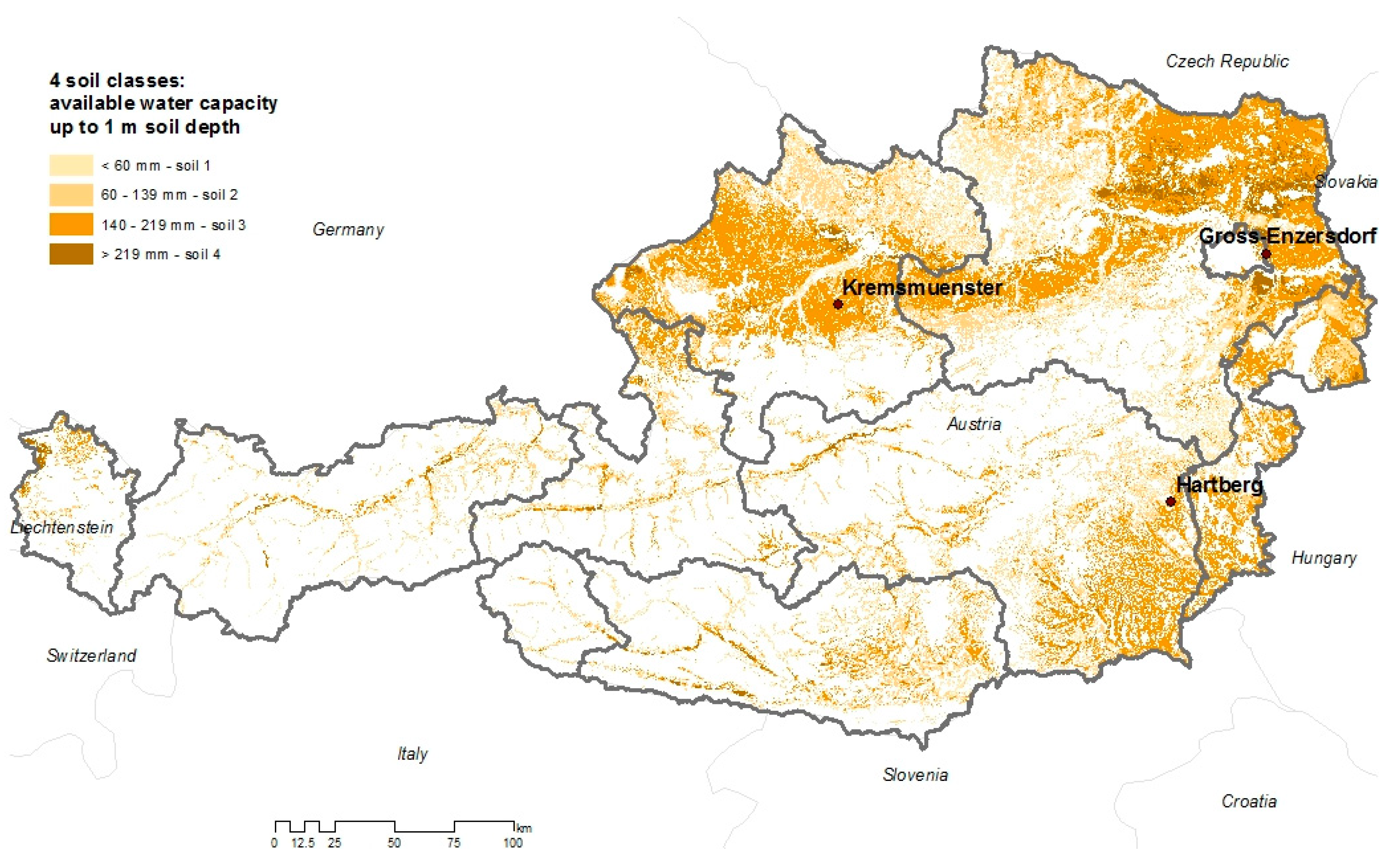
36]. In the current study, the dynamic crop growth and yield model Decision Support System for Agrotechnology Transfer (DSSAT v.4.0.2.0) [
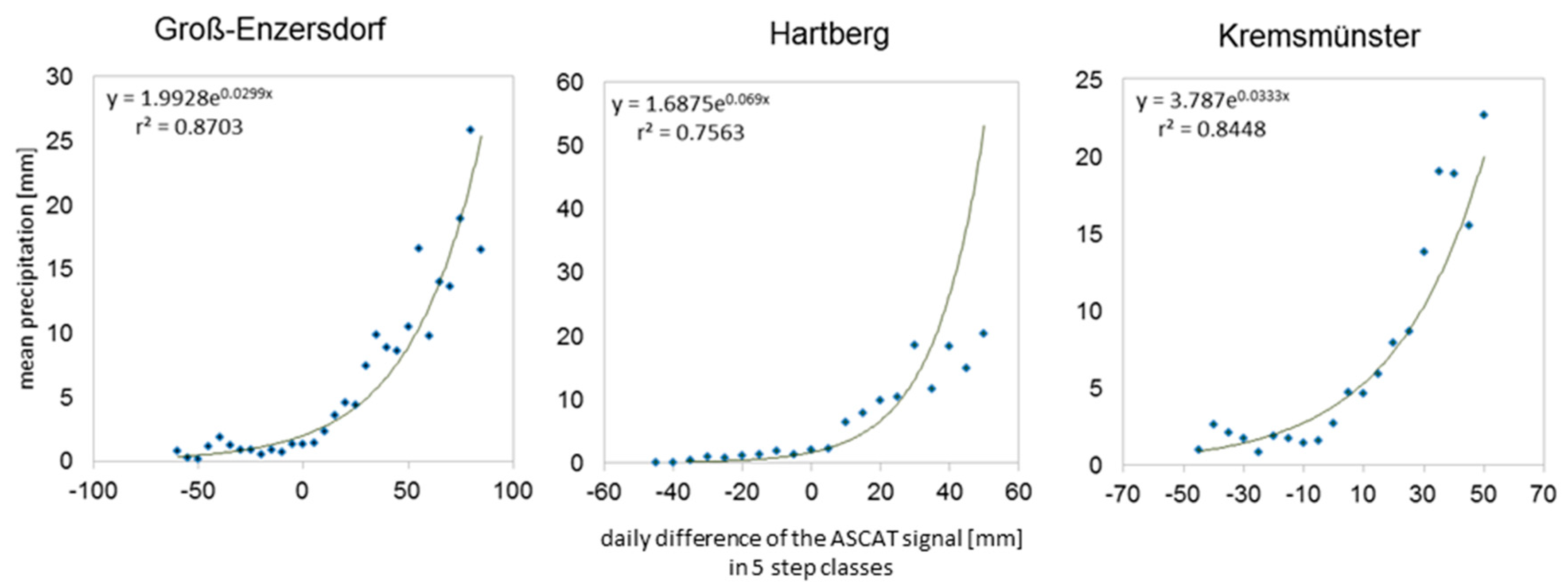
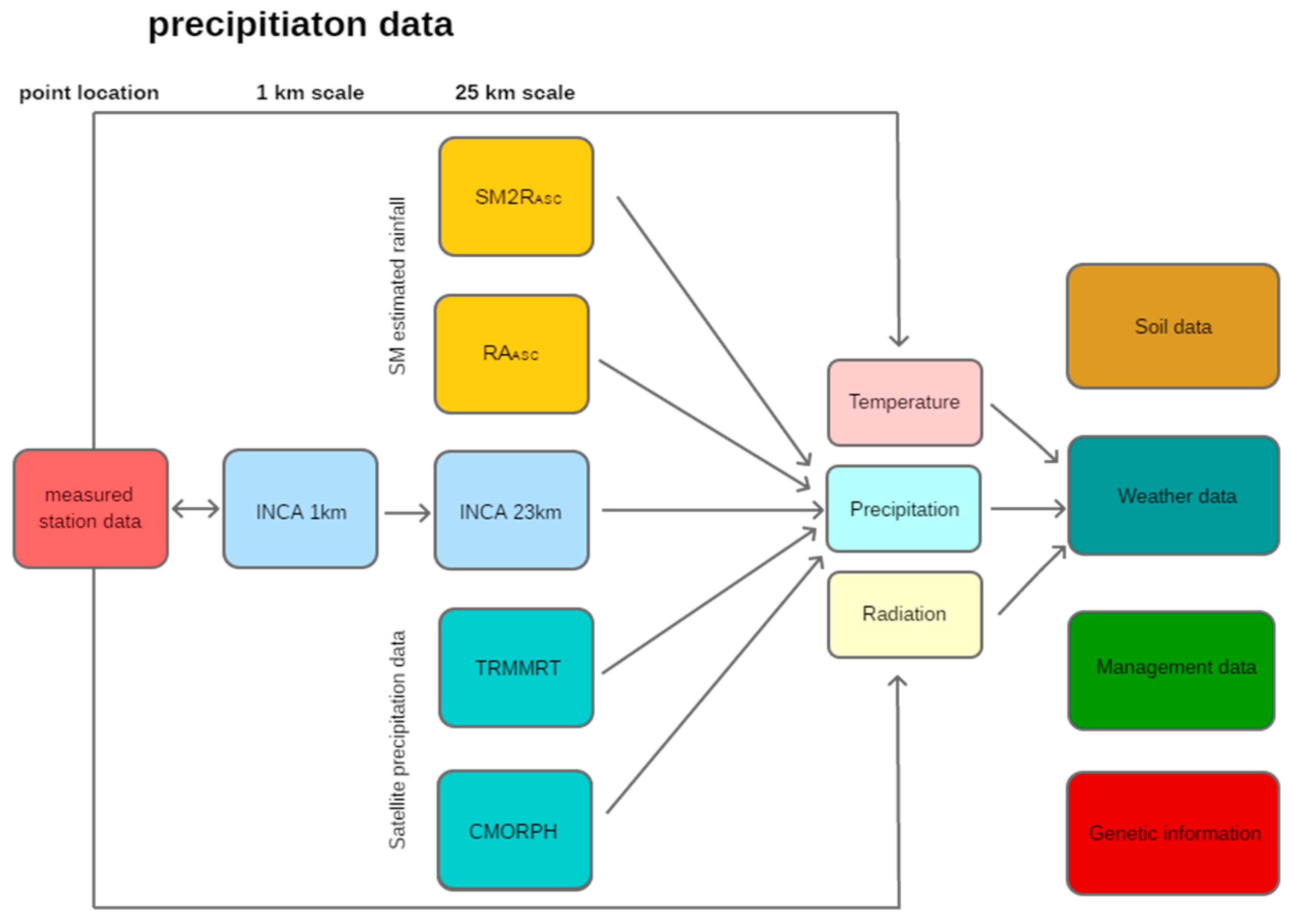
37] for wheat and barley was applied at three case study sites in Austria, characterized by different climate and soil conditions. Precipitation input data were used on the one hand as a reference from weather station-based measurements (point location) and on the other hand were compared to different types of spatial precipitation data: the data from the INtegrated Calibration and Application Tool (INCA) from the Meteorological Service Austria (1 km grid spatial resolution as well as a 25 km raster mean value), two satellite precipitation data sources—Multisatellite Precipitation Analysis (TMPA) and Climate Prediction Center MORPHing (CMORPH) with a 0.25 × 0.25° spatial resolution—a new soil moisture (SM)-derived rainfall dataset obtained through the application of the SM2RAIN algorithm [38,39] to the Metop-A/B Advanced SCATtermonter (ASCAT) soil moisture product (25 km spatial resolution) and a simple regression analysis of satellite SM data from Metop ASCAT (25 km spatial resolution). First, the performance of the different precipitation data was assessed for the three reference locations (weather station sites at each case study area). The second purpose of this study was to evaluate the consequences of the different types of precipitation data as crop model inputs, considering simulated spring barley and winter wheat yield at different soil types in the three study areas. The main aim was to test and compare whether the satellite-based precipitation data are suitable sources as input data for crop models and to identify their limitations in comparison to INCA. INCA data sets, with their high spatial resolution of 1 km, are already used as crop model inputs in Austria (for example, for the operational drought monitoring system in Austria and in research studies); however, INCA data are relatively expensive, so a survey of acceptable alternatives is of interest for several applications. Further, it is also of interest to determine under which circumstances and to which degree errors in precipitation data are propagated into final crop model results (simulated crop yield). Precipitation is the main uncertain limiting crop growth parameter over the area of interest; thus, information regarding under which conditions this important weather input parameter could be replaced by alternative spatial sources is essential.

2. Materials and Methods

2.1. Study Areas

Three sites in different climatic regions in Austria were chosen for this study (Figure 1). Groß-Enzersdorf (48°12′ N, 16°33′ E, 156 m a.s.l.) in Lower Austria is located in eastern Austria and is influenced by a semi-arid, continental climate whereabouts summers are hot and intermittently dry; winters are most of the time cold with strong frosts and rarely snow cover. The annual mean temperature in Groß-Enzersdorf from 1981–2010 was 10.3 °C and the mean annual precipitation sum was 516 mm.
Hartberg (47°17′, 15°58′ E, 359 m a.s.l.) in Styria is located in the south-eastern part of Austria and is characterized by both Mediterranean and continental climates with warm summers and mild winters. The mean average temperature was 9.4 °C and the annual precipitation sum was 716 mm (1981–2010).
Kremsmünster (48°3′ N, 14°8′ E, 384 m a.s.l.) in Upper Austria was chosen as the third site and is characterized by a central-European transition climate influenced by the Atlantic climate. It is a humid area with a moderate climate. The mean average temperature was 9.1 °C and the mean annual precipitation sum was 1003 mm (1981–2010).
These three locations, characterized by different climates, and four soil classes (Table 1, Figure 1) used in the study represent the main arable cropping areas in Austria, which occupies about 25% of the total area of Austria, quite well. We note that a high resolution and qualitative soil map is available only for the agricultural areas of Austria. Grasslands were not covered by this study.

2.2. Crop Growth Model

The DSSAT 4.0.2.0 crop model is a mechanistic or process-based, management-oriented model [37,40] and the input requirements comprehend daily weather data, soil conditions, plant characteristics, and crop management [41].
The minimum daily weather inputs for DSSAT are global solar radiation, maximum, and minimum air temperature, and precipitation [42]. These data were available from the Austrian Met Service (ZAMG) for the three weather stations Groß-Enzersdorf, Hartberg, and Kremsmünster.
Soil inputs include the soil water contents (volumetric fraction) for the lower limit of plant water availability (LL), and for the drain upper limit (DUL), where capillary forces are higher than gravity ones, and for field saturation (SAT) [42]. In the model, the FAO-56 Penman–Monteith equation [43] was used to calculate the evapotranspiration. Four different soil classes (termed here in as soil 1, soil 2, soil 3, and soil 4, respectively) were calculated from the total available water capacity (Table 1, Figure 1).
As there was no observed crop yield for all three sites available, two well calibrated crops for eastern Austria, the winter wheat cultivar “Capo” [44] and spring barley cultivar “Magda” [45], were used in this study. The simulation was set for rain-fed farming, including N fertilization (spring barley: 2 × 40 kg N/ha, 1 × 25 kg P/ha and 1 × 170 kg K/ha; winter wheat 2 × 52 kg N/ha, 1 × 26 kg P/ha and 1 × 100 K/ha), fix sowing date, harvest at maturity, and ploughed soil condition, without considering a potential yield loss provoked by pest or diseases. The sowing dates were mean values from different experimental sites of the Austrian Agency for Health and Food Safety (AGES) and were set as fixed for spring barley on March 19 in Groß-Enzersdorf and on March 24 in Hartberg as well as in Kremsmünster. For winter wheat, the dates were set on October 1 at all three locations.

2.3. Precipitation Datasets

Different spatial precipitation crop model input data were used during the 9-year period from 2007 to 2015 (Table 2): precipitation data were obtained from a nowcasting model (INCA), satellite precipitation data and rainfall estimations from SM data. All datasets were completed in the investigated period.

2.3.1. Integrated Now-Casting through Comprehensive Analysis (INCA)

INCA, a system of the Austrian Meteorological Agency (ZAMG), produces analyses and forecasts of weather parameters in a very high spatial and temporal resolution [46]. The goal of the INCA system is to provide a high-resolution weather forecast information at 1 × 1 km resolution from 6 h until 14 days. Furthermore, INCA should be more suitable for mountain landscapes, where especially attention is given to the behavior of orographic effects. The database includes topography information, more than 200 ground meteorological stations, weather radar, satellite data, and forecast models. Analyses and nowcasts are updated and produced at 1 h intervals on a horizontal resolution of 1 km and a vertical resolution of 200 m [49]. As model inputs, the INCA data at a 1 km resolution (INCA1km) were used. Additionally, the average of all 1 km INCA pixels within one ASCAT resolution cell was calculated to obtain a regional value commensurate with the ASCAT-based precipitation estimates. To simulate the ASCAT resolution cell, a Hamming window with a radius of about 23.7 km was used (INCA23km).

2.3.2. Satellite Precipitation Data

In the current study, two high-resolution satellite precipitation data sets were additionally used: the Tropical Rainfall Measurement Mission (TRMM), Multi-satellite Precipitation Analysis (TMPA) [47], and the NOAA CPC MORPHing Technique (CMORPH) [48].
The National Aeronautics and Space Administration (NASA) in cooperation with the Japan Aerospace Exploration Agency (JAXA) developed TMPA [50], a system where the estimates are reached by calibrating and merging passive microwave data and ~10 μm band infra-red (IR) data from multiple satellite sensors [51]. Six passive microwave radiometers (PMW) named the TRMM Microwave Imager (TMI), Special Sensor Microwave/Imager (SSM/I), Advanced Microwave Scanning Radiometer-EOS (AMSR-E), Advanced Microwave Sounding Unit-B (AMSU-B), Special Sensor Microwave Imager/Sounder (SSMIS), and Microwave Humidity Sounder (MHS) are utilized for rainfall estimates [50]. The IR data are accessible from the international constellation of Geosynchronous Earth Orbit (GEO) satellites [51] and contain rainfall estimates at a high spatial-temporal resolution. The product is available for the ±50° latitude band over a grid with a 0.25° spacing every 3 h [47]. In the current study, the TMPA 3B42 in real-time (RT) product, version 7, is used. Detailed information about the TMPA product can be found in Huffman et al. [47]. TMPA is hereafter referred to as TRMMRT.
CMORPH technology is developed from the NOAA/Climate Prediction Center (NOAA/CPC) and their data are available at a 0.25° × 0.25° horizontal resolution from December 2002 to the present on a 3-hourl basis [51] for the ±60° latitude band. Rainfall estimates are obtained from the same PMW radiometers (AMSU-B, SSM/I, TMI, and AMSR-E) used for retrieving TRMM rainfall estimates [48]. The dataset obtained through CMORPH v1 is hereafter referred to as CMORPH.
Both TRMMRT and CMORPH products did not use ground rainfall observations to correct satellite precipitation estimates. Diurnal accumulated precipitation was calculated by adding up rainfall estimates within one day.

2.3.3. Estimated Rainfall Based on Satellite SM Dataset

The Advanced SCATterometer (ASCAT) is a real-aperture radar instrument operating in the C-band (5.255 GHz) using vertical transmit and vertical receive (VV) polarization. ASCAT is part of the payload of a series of three Metop satellites. At the moment, Metop-A and Metop-B share the same sun-synchronous polar orbit. They were launched in October 2006 and September 2012, respectively. The last Metop satellite, Metop-C, is foreseen to be launched in October 2018, also carrying an identical ASCAT instrument [52,53]. ASCAT provides a surface soil moisture (SM) product characterized by a ~25 km (sampled at 12.5 km) and daily spatial-temporal resolution [54]. The SM product corresponds to a depth of 2–3 cm and ranges between 0% (dry) and 100% (wet) presenting the relative soil saturation [55]. A Soil Water Index (SWI) can be used to get root-zone SM information, which is a more robust product applicable for deeper soil layers and presents lower measurement noise [54].
Two approaches to estimate daily precipitation by using these satellite SM observations were used in this study, as follows:
  • An analytical relationship derived by inverting a soil–water balance equation for estimating rainfall accumulations from SM time series named SM2RAIN [38,39]. This method estimates rainfall by exploiting the knowledge about the changes in time of the amount of water stored in the soil [56]. A detailed description of the method can be found in Brocca et al. [38]. The method has been applied to several SM products and validated at different spatial/temporal scales. In the current study, the dataset obtained through the application of SM2RAIN to the ASCAT SM product was named as SM2RASC [56].
  • A direct statistical relationship between measured precipitation and the SM of the ASCAT. To estimate the daily accumulated precipitation (rainfall), the difference in ASCAT soil moisture between two consecutive days was calculated. As soon as more than one daily ASCAT SM value was available, the daily mean was used for the calculation. The daily SM differences were applied in five intervals from −100 until 100 mm, where the mean measured precipitation was added. An exponential regression analysis of these SM values (dependent variable) with the average precipitation (independent variable) in each class and each location was carried out (Figure 2). Subsequently daily precipitations were calculated with the three equations and further named as RAASC. The analyses were done for the months March until October for the period 2007–2015.

2.4. Methods Used for the Evaluation of Model Performance

Initially, a comparison of the precipitation datasets was carried out in order to evaluate the differences of the INCA1km in reference to the measured station data (point location). The analysis was done by calculating the least-squares coefficient of determination (r2), the root mean square error (RMSE), and the mean absolute error (MAE) between the daily and monthly precipitation sums.
To obtain a regional value, INCA1km was aggregated to one ASCAT resolution cell (INCA23km). Then, an evaluation of the two SM-based products and the two satellite precipitation data with INCA23km (benchmark) at the 25 km scale was carried out.
In a last step, the crop model simulations were carried out over a 9-year period covering 2007–2015 for five different daily precipitation model inputs; as references, daily precipitation data from INCA23km were used. Furthermore, SM2RASC, RAASC, TRMMRT, and CMORPH were used as forcing variables, respectively (Figure 3). These rain data were utilized only for the months March until October, as satellite soil moisture retrievals are influenced by the presence of snow and frozen surfaces [57]. From November until February, INCA23km rainfall data was used. To assess and compare model performance, a set of statistical parameters was calculated: the mean absolute error (MAE), the root mean square error (RMSE), the percent bias (PBias), the index of agreement (d), and the least-squares coefficient of determination (r2).

3. Results

3.1. Rainfall Datasets Comparison

The daily and monthly precipitation differences between point-measured (ZAMG) and areal estimates from INCA1km for the months March until July and years 2007–2015 are shown in Table 3. For the evaluation, only five months per year were considered, as they include the main growing period of the two simulated crops, spring barley and winter wheat. Trends during the growing season period (March until July) were estimated on a monthly scale to get the temporal variability of the product performance by calculating r2, RMSE, and MAE. INCA1km performs very well with an r2 greater than 0.69 (diurnal) and 0.89 (by the month), respectively, as well as a daily RMSE < 4 mm and monthly RMSE < 18 mm. The daily MAE is between 0.7 and 1.4 mm, the monthly one between 8.5 and 17.7 mm. It should be kept in mind that INCA1km also integrates the ground measurements to estimate the gridded precipitation values.
To evaluate values in the same spatial resolution, and due to the good accordance of INCA1km and ZAMG precipitation values, INCA data were next aggregated to the 25 km scale. The aggregated INCA23km presents in all three locations a higher precipitation sum (monthly and daily) and is particularly pronounced in the first three months of the study in all three locations (except Groß-Enzersdorf in April and Kremsmünster in March) (Table 4).
In a next step, the two SM-based products SM2RASC, and RAASC, as well as the two satellite precipitation datasets TRMMRT and CMORPH, were compared with INCA23km (benchmark) in terms of rainfall estimation (daily: Table 5, monthly: Figure 4).
The lowest r2 can be seen in the RAASC daily and monthly precipitation data. RAASC is characterized by high values during low precipitation periods and by lower values in very humid months (Figure 4). The other three approaches show—for the most part—a good coefficient of determination (up to 0.52 daily and 0.68 monthly) with INCA23km. One exception is SM2RASC in Kremsmünster, where it shows high deviations and presents weak monthly performance results (r2 = 0.18 and RMSE = 60 mm). The two SM-based products present a low root-mean-square error in Groß-Enzersdorf; in the other two locations RMSE differences between SM-based products and satellite precipitation data are smaller (Table 5, Figure 4).
The number of rain days alone was not considered in this study as a main crucial factor for crop water balance in Austria, as factors such as actual evapotranspiration affecting soil water balance are omitted. More important is the soil available water capacity for the plants and its dynamics on a daily basis, which is used in this study as the best estimator of crop water stress available; e.g., [43].

3.2. Crop Model Performance

The influence of four different forcing variables (2 SM-based products SM2RASC and RAASC, 2 satellite precipitation data TRMMRT, and CMORPH) were used as an input on the DSSAT model in order to evaluate their impact on spring barley and winter wheat yield estimations in comparison to the benchmark (INCA23km).

3.2.1. Spring Barley

The growing season for spring barley reaches from March until July. The sowing date was set as fixed (see Section 2.2) and the 9-year mean flowering was simulated between 5 and 9 June and mean maturity from 30 June (Groß-Enzersdorf) until 5 July (Kremsmünster). The mean spring barely yield over all soil classes (soils 1–4) was simulated in Groß-Enzersdorf with around 4700 kg/ha, in Hartberg around 5100 kg/ha, and in Kremsmünster 4400 kg/ha (Table 6).
A detailed comparison of the spring barley yield, estimated with INCA23km input (benchmark), showed that none of the other grid precipitation inputs perfectly reproduced the simulated yields in all years (Figure 5, Table 6). The analyses were carried out for all soil types together (soils 1–4) as well as separately (soil 1, soil 2, soil 3, and soil 4).
In the semi-arid area of Groß-Enzersdorf, the different types of precipitation inputs caused the highest deviations, where mainly light-textured soils (soil classes 1 and 2 with mostly RMSE > 600 kg/ha) are more sensitive than moderately fine-textured soils (soil classes 3 and 4) (Figure 4, Table 3). SM2RASC generally presented the highest MAE (soil 1–4 = 512 kg/ha) and RMSE values (soil 1–4 = 633 kg/ha), whereas CMORPH showed the lowest one (soil 1–4 = 431 kg/ha). It is also noticeable that SM2RASC and CMORPH underestimated the barley yield (negative PBias), where RAASC and TRMMRT input data demonstrated a positive PBias (Table 3).
Lower yield differences were found in the more humid areas of Hartberg and Kremsmünster with all precipitation inputs—especially for soils 3 and 4 (Figure 4). It can be notice, that the RMSE values in these two locations are about less than half that in Groß-Enzersdorf. Above all, TRMMRT presents very low MAE and RMSE values in Hartberg (MAE: soil 1–4 = 135 kg/ha; RMSE: soil 1–4 = 174 kg/ha) and the highest r2 (soil 1–4 = 99%) as well as d (soil 1–4 = 96%). CMORPH, on the other hand, shows difficulties to simulate yield in Kremsmünster, which is characterized by the highest RMSE (soil 1–4 = 602 kg/ha) and the weakest coefficient of determination (soil 1–4 = 82%) as well as index of agreement (soil 1–4 = 62%) (Table 3). The light-textured soils result in all simulations in a negative PBias; soils 3 and 4 do not show such a clear trend.

3.2.2. Winter Wheat

The winter wheat phenological season spans from October until July, including a dormant period during winter. The sowing date was set as fixed on October 1 and the 9-year mean flowering date was simulated between 27 and 30 May, with mean maturity between 28 June and 3 July. The mean yield for all soil types together (soils 1–4) was simulated between 5500 kg/ha in Kremsmünster and 5900 kg/ha in Hartberg (Table 7).
The variation of winter wheat yields, as a result of different precipitation input data, illustrated a similar behavior to the spring barley simulations.
Groß-Enzersdorf presented the highest winter wheat yield deviations (Figure 5)—especially for soil classes 1 and 2, with RMSE values up to 1800 kg/ha. The outlier in soil 1 was caused in year 2011, where INCA23km input data simulated yield failure. SM2RASC, TRMMRT, and CMORPH mainly underestimated yield, whereas RAASC presented a positive PBias (Figure 5, Table 4). All in all, RAASC showed the strongest performances, with the lowest RMSE (soil 1–4 = 818 kg/ha) and a high d (soil 1–4 = 0.94) as well as r2 (soil 1–4 = 0.84).
In the two locations Hartberg and Kremsmünster, lower deviations can be seen (Figure 6). Notable are the TRMMRT input data, which simulated winter wheat yield in Hartberg (RMSE soil 1–4 = 194 kg/ha; d > 95%) and SM2RASC in Kremsmünster (RMSE soil 1–4 = 223 kg/ha, d > 95%) very well (Table 4). CMORPH input data caused the highest deviations and the poorest performances. All four rainfall input data showed a yield underestimation (negative PBias) (Table 4).

4. Discussion

Crop growth simulation models are increasingly being utilized as tools to assess the regional impact on crop production under different environmental conditions, such as changing climate and management options. These models need spatially and temporally detailed input data of weather, soil, crop management, and cultivar, which are usually difficult to get reliably for larger areas [58]. As observation data are merely available at a limited number of meteorological stations within a region, it is essential to estimate the required weather inputs for the related simulation-scale [59]. The focus of this study was set on daily precipitation data, as they are the main uncertain limiting crop growth parameter over the area of interest. Crop models are highly sensitive to soil water, as soil moisture is a limiting factor for different processes for crop growth and yield. A valued alternative to ground-based measurements can be satellite-rainfall estimate systems, which produce global coverage data and supply information in areas where data from other sources are unavailable [60]. The spatial and temporal resolution increased lately; e.g., the current NASA–JAXA joint Global Precipitation Measurement (GPM) mission makes available rainfall products in near-real time with a spatial sampling of 0.1° each 30 min, by utilizing different satellite sensors [61]. Satellite rainfall products which have been previously developed include the near-real-time TMPA 3B42RT [48]; the Precipitation Estimation from Remotely Sensed Information using Artificial Neural Networks (PERSIANN) [62]; CMORPH [49]; and the Climate Hazards Group InfraRed Precipitation with Station (CHIRPS) products [63]. Nevertheless, satellite rainfall estimations are not free of error [64,65]. One main reason is the inconsistent scan of rainfall patterns, which makes the reconstruction of the accumulated rainfall in longer temporal scales (e.g., daily accumulated rainfall) challenging [66]. Further, the estimation of light rainfall is generally underestimated especially over land by remote sensing analyses as a result of land surface emissivity [36,60,67].
Approaches to enhance the quality of satellite rainfall estimates, the use of satellite surface soil moisture (SSM) data has been utilized recently [38,39,68,69,70,71]. These methods analyze the intense correlation between SSM and rainfall to improve and/or estimate rainfall by using satellite surface SM data. Here, SM2RAIN [38] is the first method, which directly makes available rainfall estimates from SSM observations, whereas the other approaches are correction-based techniques [36,38,39,60,72,73,74,75]. In our study, we also added a new approach to estimate rainfall directly using the statistical relationship between measured precipitation and the SM of the ASCAT.
Meteorological station data are normally spatially irregular and can be interpolated to a regular grid. At this point, especially high-resolution gridded data sets can be used for impact studies. Examples are the EURO4M-APGD dataset for the Alps [76], the European E-OBS [77], and JRC’s Agri4cast dataset (http://agri4cast.jrc.ec.europa.eu). These data were not analyzed in the current study. Here (e.g., for Austria), INCA data exists with a very high-resolution gridded data set; unfortunately, they are not freely available.
An important aspect of crop models is that they are sensitive to perturbations in precipitation. In Eitzinger et al. [78], the sensitivity of seven different crop models for winter wheat and maize to extreme heat and drought over a short but critical period of two weeks after the start of flowering in two locations in Austria was studied. It showed, that the models respond differently to climate stresses (according to references [79,80]), even though they mainly present similar trends in grain yields between different climatic situations. In Fronzek et al. [81], process-based wheat models were applied, and no single model property was found, which describe the combined yield response to temperature and precipitation perturbations.
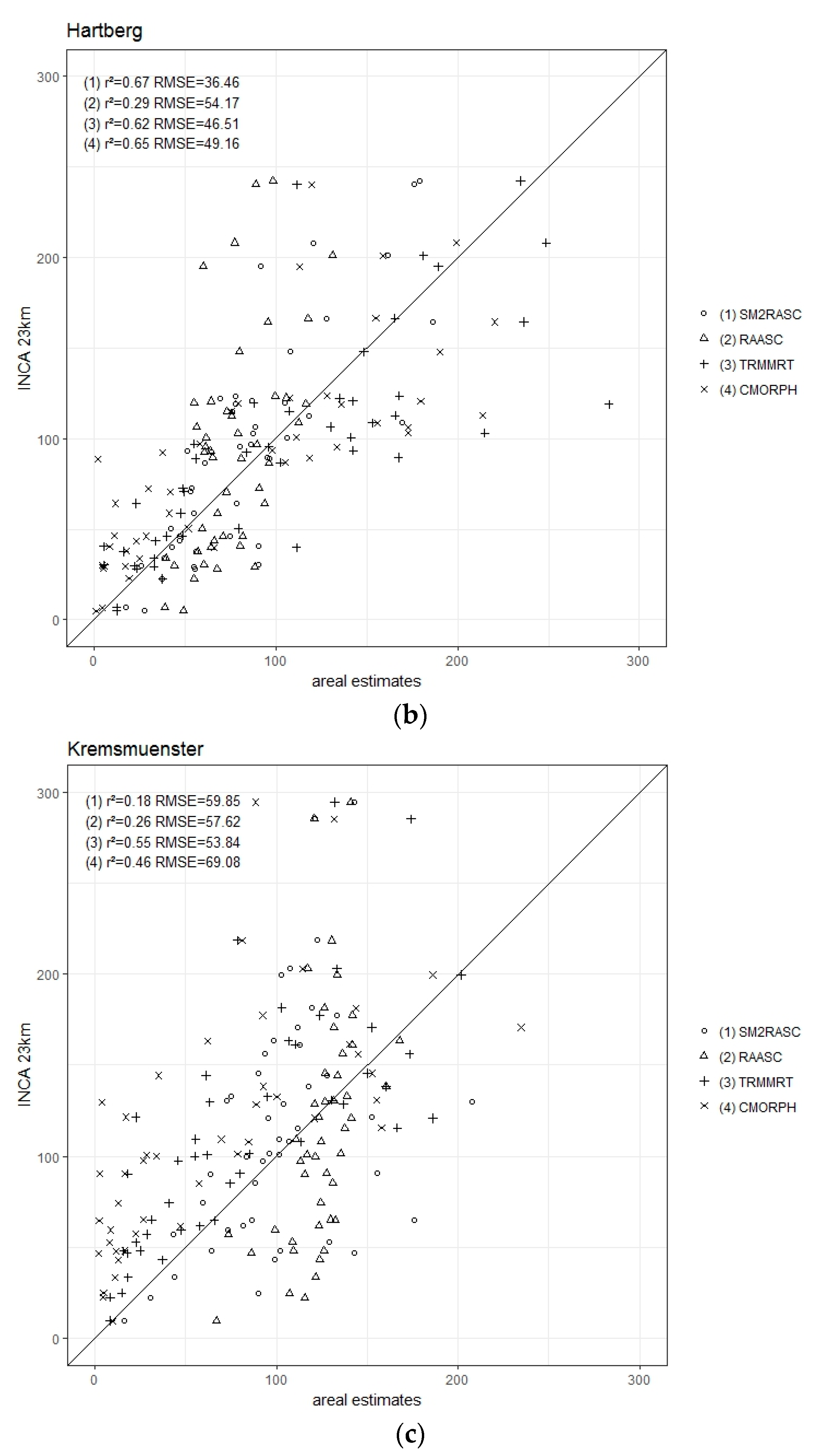
The main objective of the current study was to test different types of spatial precipitation data as inputs for a crop model application in three locations in Austria with different soil types and climates. As INCA data are not freely available, a study of acceptable spatial alternatives is of interest for serval applications. Also, under which circumstances and to which degree errors in precipitation data are propagated into final crop model results are of interest. Therefore, the aggregated INCA23km presented in all three locations already a higher precipitation sum as INCA1km and were thus not free of errors.
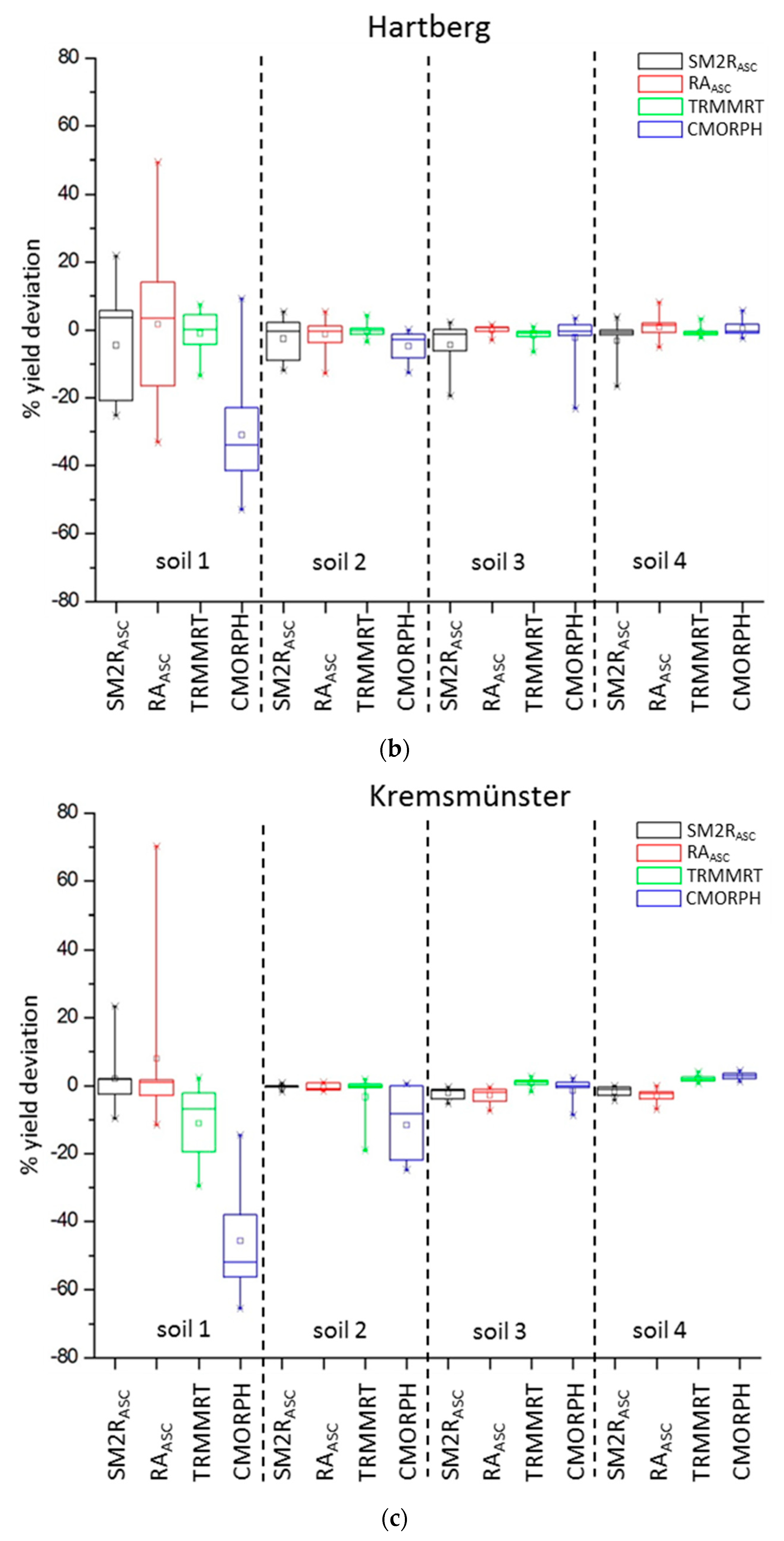
All investigated grid-based types of precipitation data perform at their best as crop yield model inputs on moderately fine-textured soils and under humid conditions (Hartberg and Kremsmünster).
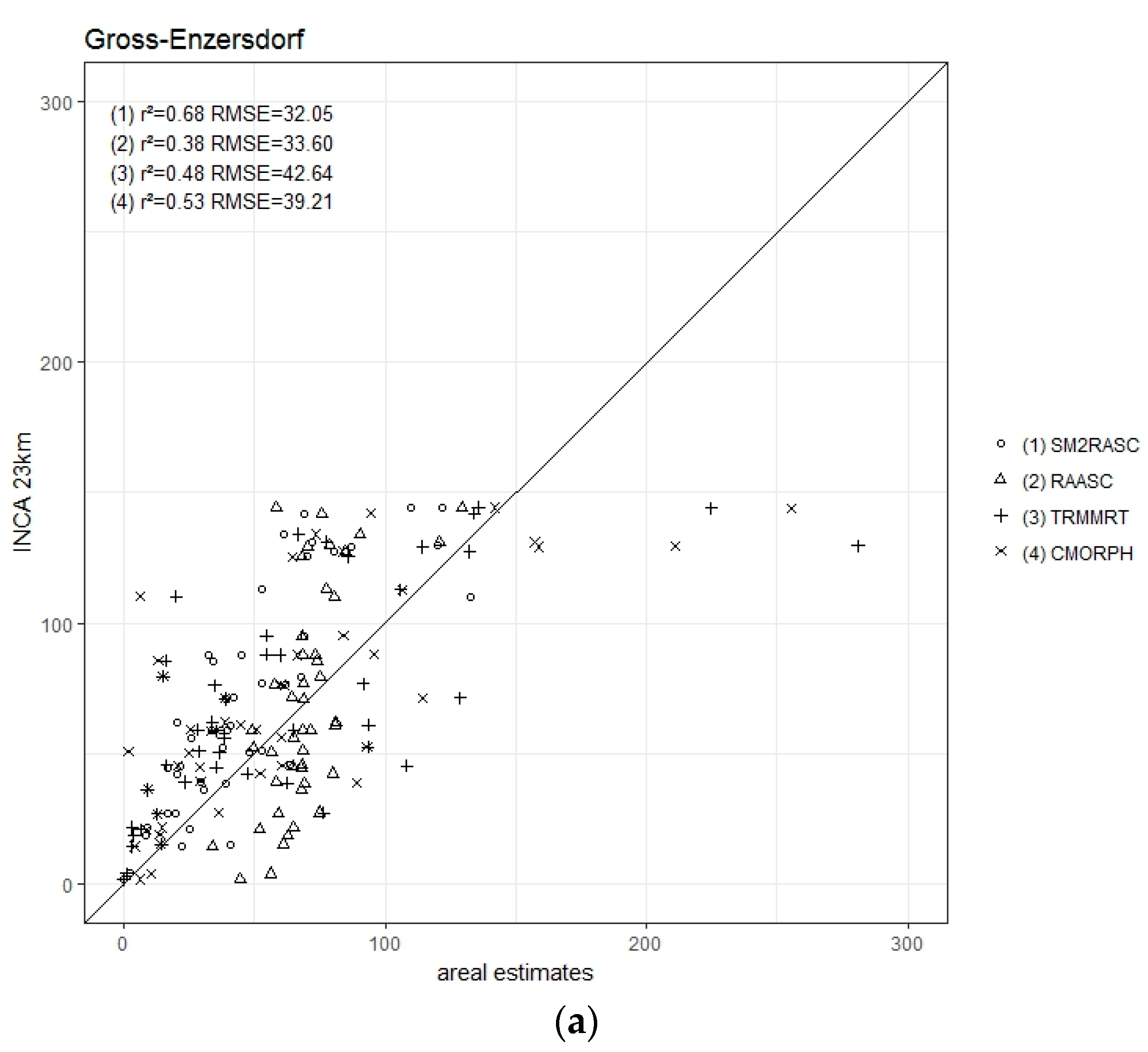
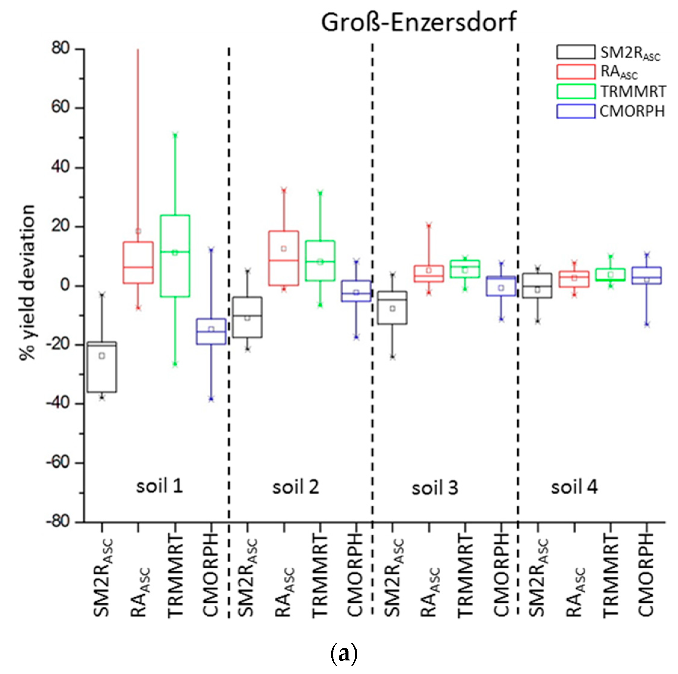
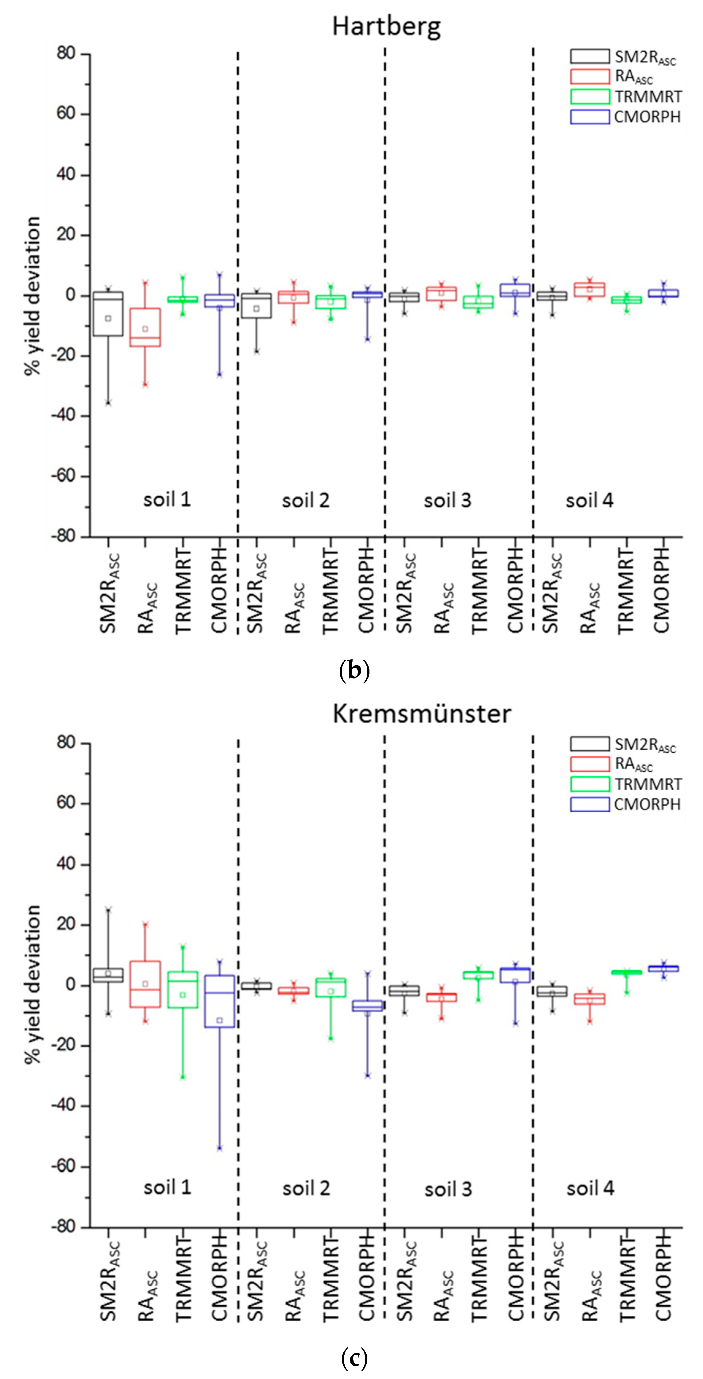
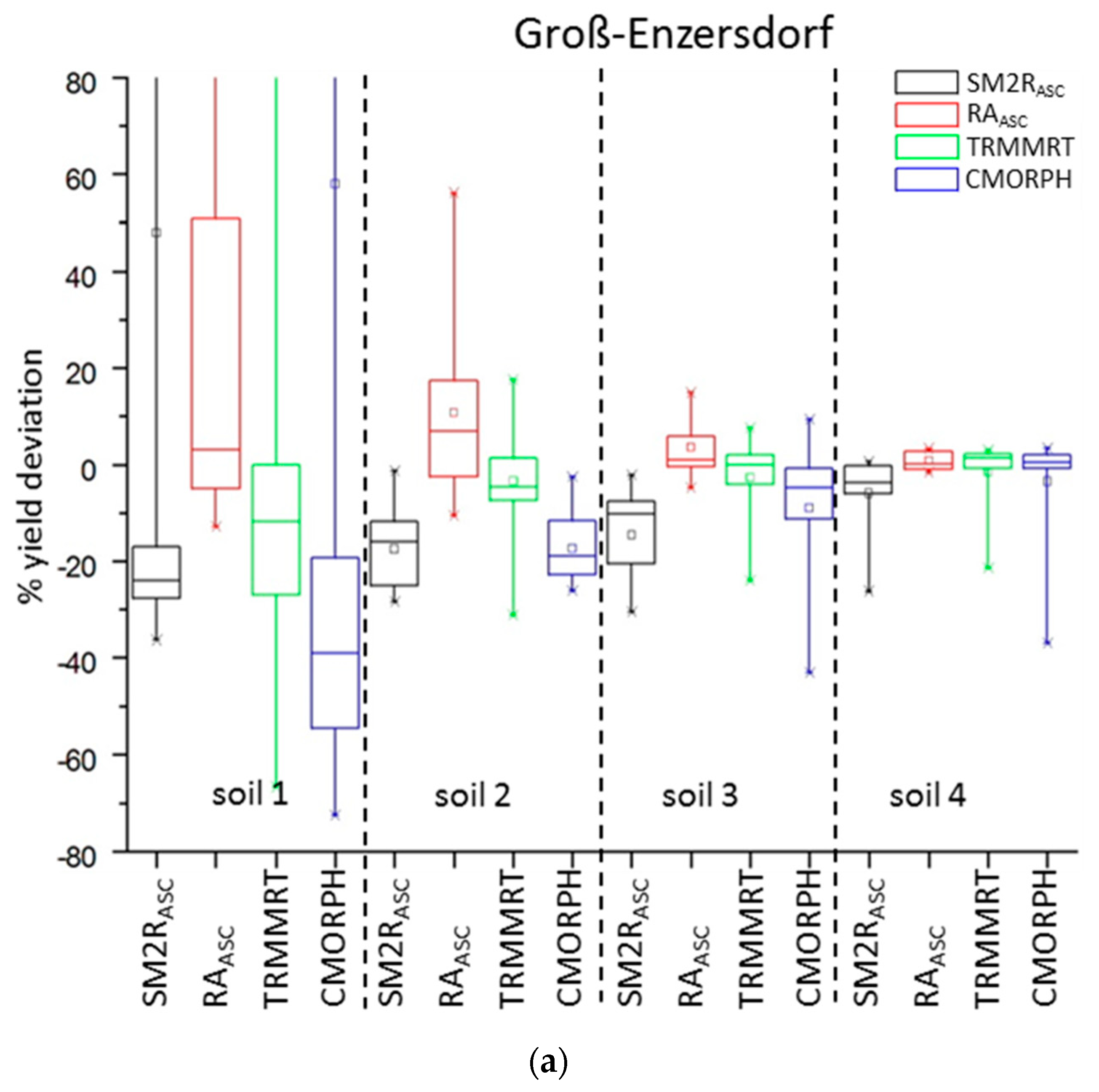
In the semi-arid region of Groß-Enzersdorf, winter wheat and spring barley simulations are very sensitive to different precipitation model inputs; especially in light-textured soils. This is due to the fact that soil water availability is a more dominant limiting growth factor under drought-prone conditions. Therefore, little differences in precipitation input can affect greatly the simulated yield (high RMSE, low d and r2 values). Also, even one missing precipitation event in a critical development stage can cause a crop failure. In this region, the model reacts more sensitively for winter wheat than for spring barley. RAASC (winter wheat) and TRMMRT (winter wheat and spring barley) seem to be the best predictors for this location.
In the more humid places of Hartberg and Kremsmünster, all four precipitation inputs produced good agreements. Plant water stress does not occur often and can be observed mainly in light-textured soils. A bias in the precipitation sum is not such a crucial factor here; much more important is a prediction of the event. In Hartberg, crop yields with RAASC and TRMMRT input data correspond best with INCA23km input data (except RAASC soil 1). In Kremsmünster, both SM-based products present good yield results for soils 1 and 2; even if high monthly precipitation differences to INCA23km were calculated (Figure 3). Winter wheat and spring barley show similar yield predictions in both locations.
The poorest performances in all three locations and for both crops were found with CMORPH input data. The general underestimation of rainfall provided by CMORPH is in line with the finding of Stampoulis and Anagnostou [82], who assess the quality of this product over Europe.
Looking at SM estimated rainfall in more detail, SM2RASC and RAASC perform well in this study, especially on light-textured soils in Kremsmünster and Hartberg compared to the two satellite precipitation data. Here, for example, the use of information regarding the spatial–temporal variability of top soil moisture could improve spatial crop yield simulations against the use of single point information for single weather stations for a given area. Therefore, the SM estimations (SM2RASC, RAASC) could be an alternative for potential agriculture applications in regions where other products are not available once calibrated to the specific climatic conditions. In addition, a remote sensing product does not necessarily have to be “better” than the model. It should be considered whether the data add value or new information. Hence, even when r2 values are lower than for models, clever data assimilation approaches may take advantage of the data (see e.g., [28]).

5. Conclusions

In the current study, different types of spatial precipitation data as inputs were tested for a crop model application. Two daily satellite precipitation and two estimated rainfall data based on a satellite SM dataset were evaluated with INCA-input data at a spatial resolution of around 25 km in three locations in Austria. A bias in precipitation model input has lower impacts on simulated spring barley and winter wheat yield under humid (Kremsmünster and Hartberg) than under dry conditions (Groß-Enzersdorf). This can be very well observed in TMPA and in the two SM-based product simulations. Additionally, light-textured soils (especially soil class 1) show more sensitivity to different precipitation inputs than the other soils, regardless of the studied region.
This study represents one of the first attempts to integrate estimated rainfall datasets from SM for crop models. More comprehensive analyses will be approached henceforth in order to better understand and improve the capability of satellite-derived rainfall.

Author Contributions

The work has been performed in collaboration with all co-authors. S.T. and J.E. conceived the research. L.B. and L.C. provided SM2RASC data as well as the two satellite precipitation data. S.H. and W.W. provided the daily ASCAT SM data. S.T. performed the statistical analysis and prepared the manuscript. A critical analysis of obtained results, reading, and commenting of the manuscript throughout all processes were done of all authors.

Funding

This research was funded by the European Unions Horizon 2020 research and innovation programme grant number 691998.

Acknowledgments

This paper is supported by the H2020-TWINN-2015 SERBIA FOR EXCELL project. This project has received funding from the European Unions Horizon 2020 research and innovation programme under grant agreement No. 691998. The work described in this paper was realized as a part of the project “COMBIRISK” of the Austrian Climate Research Programme (ACRP).

Conflicts of Interest

The authors declare no conflict of interest.

References

  1. Penning de Vries, F.W.T.; Jansen, D.M.; ten Berge, H.F.M.; Bakema, A. Simulation of Ecophysiological Processes of Growth in Several Annual Crops; Centre for Agricultural Publishing and Documentation (Pudoc): Wageningen, The Netherlands, 1989. [Google Scholar]
  2. Dadhwal, V.K. Crop growth and productivity monitoring and simulation using remote sensing and GIS. In Satellite Remote Sensing and GIS Applications in Agricultural Meteorology, Proceedings of the Training Workshop, Dehra Dun, India, 7–11 July 2003; Sivakumar, M.V.K., Roy, P.S., Harmsen, K., Saha, S.K., Eds.; World Meteorological Organization: Geneva, Switzerland, 2003; pp. 263–290. [Google Scholar]
  3. De Wit, A.J.W.; Boogaard, H.L.; van Diepen, C.A. Spatial resolution of precipitation and radiation: The effect on regional crop yield forecasts. Agric. For. Meteorol. 2005, 135, 156–168. [Google Scholar] [CrossRef]
  4. Delécolle, R.; Maas, S.J.; Guerif, M.; Baret, F. Remote sensing and crop production models: Present trends. ISPRS J. Photogramm. Remote Sens. 1992, 47, 145–161. [Google Scholar] [CrossRef]
  5. Ewert, F.; van Ittersum, M.K.; Heckelei, T.; Therond, O.; Bezlepkina, I.; Andersen, E. Scale changes and model linking methods for integrated assessment of agri-environmental systems. Agric. Ecosyst. Environ. 2011, 142, 6–17. [Google Scholar] [CrossRef]
  6. De Wit, A.J.W.; van Diepen, C.A. Crop growth modelling and crop yield forecasting using satellite-derived meteorological inputs. Int. J. Appl. Earth Obs. Geoinf. 2008, 10, 414–442. [Google Scholar] [CrossRef]
  7. De Wit, A.; Baruth, B.; Boogaard, H.; van Diepen, K.; van Kraalingen, D.; Micale, F.; te Roller, J.; Supit, I.; van den Wijngaart, R. Using ERA-INTERIM for regional crop yield forecasting in Europe. Clim. Res. 2010, 44, 41–53. [Google Scholar] [CrossRef] [Green Version]
  8. Ma, H.; Huang, J.; Zhu, D.; Liu, J.; Zhang, C.; Su, W.; Fan, J. Estimating regional winter wheat yield by assimilation of time series of HJ-1 CCD into WOFOST-ACRM model. Math. Comput. Model. 2013, 58, 753–764. [Google Scholar] [CrossRef]
  9. Patel, N.R.; Mandal, U.K.; Pande, L.M. Agro-ecological zoning system. A Remote Sensing and GIS Perspective. J. Agrometeorol. 2000, 2, 1–13. [Google Scholar]
  10. Ismail, M. Using Remote Sensing and GIS Application in Agro-ecological Zoning of Egypt. Int. J. Environ. Sci. 2012, 1, 85–94. [Google Scholar]
  11. Taati, A.; Sarmadian, F.; Mousavi, A.; Rahmani, A. Agro-ecological zoning for cultivation of Alfalfa (Medicago sativa L.) using RS and GIS. Sci. Agric. 2015, 9, 93–100. [Google Scholar] [CrossRef]
  12. Mustak, S.K.; Baghmar, N.K.; Singh, S.K. Land Suitability Modeling for gram crop using remote sensing and GIS: A case study of Seonath basin, India. Bull. Environ. Sci. Res. 2015, 4, 6–17. [Google Scholar]
  13. Kamau, S.W.; Kuria, D.; Gachari, M.K. Crop-land Suitability Analysis Using GIS and Remote Sensing in Nyandarua County, Kenya. J. Environ. Earth Sci. 2015, 5, 121–131. [Google Scholar]
  14. Mustafa, A.A.; Singh, M.; Sahoo, R.N.; Ahmed, N.; Khanna, M.; Sarangi, A.; Mishra, A.K. Land Suitability Analysis for Different Crops: A Multi Criteria Decision Making Approach using Remote Sensing and GIS. Researcher 2011, 3, 61–84. [Google Scholar]
  15. Lobell, D.B. The use of satellite data for crop yield gap analysis. Field Crop. Res. 2013, 143, 56–64. [Google Scholar] [CrossRef]
  16. Sibley, A.M.; Grassini, P.; Thomas, N.E.; Cassman, K.G.; Lobell, D.B. Testing Remote Sensing Approaches for Assessing Yield Variability among Maize Fields. Agron. J. 2014, 106, 24–32. [Google Scholar] [CrossRef] [Green Version]
  17. Seelan, S.K.; Laguette, S.; Casady, G.M.; Seielstad, G.A. Remote sensing applications for precision agriculture: A learning community approach. Remote Sens. Environ. 2003, 88, 157–169. [Google Scholar] [CrossRef]
  18. Mulla, D.J. Twenty five years of remote sensing in precision agriculture: Key advances and remaining knowledge gaps. Biosyst. Eng. 2013, 114, 358–371. [Google Scholar] [CrossRef]
  19. Dorigo, W.A.; Zurita-Milla, R.; de Wit, A.J.; Brazile, J.; Singh, R.; Schaepman, M.E. A review on reflective remote sensing and data assimilation techniques for enhanced agroecosystem modeling. Int. J. Appl. Earth Obs. Geoinf. 2007, 9, 165–193. [Google Scholar] [CrossRef]
  20. Morel, J.; Begue, A.; Todoroff, P.; Martine, J.; Lebourgeois, V.; Petit, M. Coupling a sugarcane crop model with the remotely sensed time series of fIPAR to optimise the yield estimation. Eur. J. Agron. 2014, 61, 60–68. [Google Scholar] [CrossRef]
  21. Moulin, S.; Bondeau, A.; Delécolle, R. Combining agricultural crop models and satellite observations: From field to regional scales. Int. J. Remote Sens. 1998, 19, 1021–1036. [Google Scholar] [CrossRef]
  22. Launay, M.; Guerif, M. Assimilating remote sensing data into a crop model to improve predictive performance for spatial applications. Agric. Ecosyst. Environ. 2005, 111, 321–339. [Google Scholar] [CrossRef]
  23. De Wit, A.J.W.; Van Diepen, C.A. Crop model data assimilation with the Ensemble Kalman filter for improving regional crop yield forecasts. Agric. For. Meteorol. 2007, 146, 38–56. [Google Scholar] [CrossRef]
  24. Fang, H.; Liang, S.; Hoogenboom, G.; Teasdale, J.; Cavigelli, M. Corn-yield estimation through assimilation of remotely sensed data into the CSM-CERES-Maize model. Int. J. Remote Sens. 2008, 29, 3011–3032. [Google Scholar] [CrossRef]
  25. Dong, Y.; Zhao, C.; Yang, G.; Chen, L.; Wang, J.; Feng, H. Integrating a very fast simulated annealing optimization algorithm for crop leaf area index variational assimilation. Math. Comput. Model. 2013, 58, 877–885. [Google Scholar] [CrossRef]
  26. Li, Y.; Zhou, Q.; Zhou, J.; Zhang, G.; Chen, C.; Wang, J. Assimilating remote sensing information into a coupled hydrology-crop growth model to estimate regional maize yield in arid regions. Ecol. Model. 2014, 291, 15–27. [Google Scholar] [CrossRef]
  27. Jongschaap, R.E. Run-time calibration of simulation models by integrating remote sensing estimates of leaf area index and canopy nitrogen. Eur. J. Agron. 2006, 24, 316–324. [Google Scholar] [CrossRef]
  28. Draper, C.S.; Reichle, R.H.; De Lannoy, G.J.M.; Liu, Q. Assimilation of passive and active microwave soil moisture retrievals. Geophys. Res. Lett. 2012, 39, L04401. [Google Scholar] [CrossRef]
  29. Thorp, K.R.; Wang, G.; West, A.L.; Moran, M.S.; Bronson, K.F.; White, J.W.; Mon, J. Estimating crop biophysical properties from remote sensing data by inverting linked radiative transfer and ecophysiological models. Remote Sens. Environ. 2012, 124, 224–233. [Google Scholar] [CrossRef] [Green Version]
  30. Li, Z.; Jin, X.; Zhao, C.; Wang, J.; Xu, X.; Yang, G.; Li, C.; Shen, J. Estimating wheat yield and quality by coupling the DSSAT-CERES model and proximal remote sensing. Eur. J. Agron. 2015, 71, 53–62. [Google Scholar] [CrossRef]
  31. Wiegand, C.L.; Richardsons, A.J.; Kanemasu, E.T. Leaf area index estimates for wheat from LANDSAT and their implications for evapotranspiration and crop modeling. Agron. J. Abstr. 1979, 71, 336–342. [Google Scholar] [CrossRef]
  32. Richardson, A.J.; Wiegand, C.L.; Arkin, G.F.; Nixon, P.R.; Gerbermann, A.H. Remotely sensed spectral indicators of sorghum development and their use in growth modelling. Agric. Meteorol. 1982, 26, 11–23. [Google Scholar] [CrossRef]
  33. Reynolds, C.A.; Yitayew, M.; Slack, D.C.; Hutchinson, C.F.; Huete, A.; Peterson, M.S. Estimating crop yields and production by integrating the FAO Crop Specific Water Balance model with real-time satellite data and ground-based ancillary data. Int. J. Remote Sens. 2000, 21, 3487–3508. [Google Scholar] [CrossRef]
  34. Ovando, G.; Sayago, S.; Bocco, M. Evaluating accuracy of DSSAT model for soybean yield estimation using satellite weather data. ISPRS J. Photogramm. Remote Sens. 2018, 138, 208–217. [Google Scholar] [CrossRef]
  35. Dinku, T.; Ceccato, P.; Grover-Kopec, E.; Lemma, M.; Connor, S.J.; Ropelewsky, C.F. Validation of satellite rainfall products over East Africa’s complex topography. Int. J. Remote Sens. 2007, 28, 1503–1526. [Google Scholar] [CrossRef]
  36. Ciabatta, L.; Brocca, L.; Massari, C.; Moramarco, T.; Puca, S.; Rinollo, A.; Gabellani, S.; Wagner, W. Integration of satellite soil moisture and rainfall observations over the Italian territory. J. Hydrometeorol. 2015, 16, 1341–1355. [Google Scholar] [CrossRef]
  37. Jones, J.W.; Hoogenboom, G.; Porter, C.H.; Boote, K.J.; Batchelor, W.D.; Hunt, L.A.; Wilkens, P.W.; Singh, U.; Gijsman, A.J.; Ritchie, J.T. The DSSAT cropping system model. Eur. J. Agron. 2003, 18, 235–265. [Google Scholar] [CrossRef]
  38. Brocca, L.; Moramarco, T.; Melone, F.; Wagner, W. A new method for rainfall estimation through soil moisture observations. Geophys. Res. Lett. 2013, 40, 853–858. [Google Scholar] [CrossRef] [Green Version]
  39. Brocca, L.; Ciabatta, L.; Massari, C.; Moramarco, T.; Hahn, S.; Hasenauer, S.; Kidd, R.; Dorigo, W.; Wagner, W.; Levizzani, V. Soil as a natural rain gauge: Estimating global rainfall from satellite soil moisture data. J. Geophys. Res. Atmos. 2014, 119, 5128–5141. [Google Scholar] [CrossRef] [Green Version]
  40. Jones, J.W.; Keating, B.A.; Porter, C.H. Approaches to modular model development. Agric. Syst. 2001, 70, 241–443. [Google Scholar] [CrossRef]
  41. Hunt, L.A.; White, J.W.; Hoogenboom, G. Agronomic data: Advances in documentation and protocols for exchange and use. Agric. Syst. 2001, 70, 477–492. [Google Scholar] [CrossRef]
  42. Singh, A.K.; Tripathy, R.; Chopra, U.K. Evaluation of CERES-Wheat and CropSyst models for water-nitrogen interactions in wheat crop. Agric. Water Manag. 2008, 95, 776–786. [Google Scholar] [CrossRef]
  43. Allen, G.A.; Pereira, L.S.; Raes, D.; Smith, M. Crop Evapotranspiration: Guidelines for Computing Crop Water Requirements, Irrigation and Drainage Paper No. 56; FAO: Rome, Italy, 1998. [Google Scholar]
  44. Thaler, S.; Eitzinger, J.; Trnka, M.; Dubrovsky, M. Impacts of climate change and alternative adaptation options on winter wheat yield and water productivity in a dry climate in Central Europe. J. Agric. Sci. 2012, 150, 537–555. [Google Scholar] [CrossRef]
  45. Eitzinger, J.; Trnka, M.; Semerádová, D.; Thaler, S.; Svobodová, E.; Hlavinka, P.; Siska, B.; Takác, J.; Malatinská, L.; Nováková, M.; et al. Regional climate change impacts on agricultural crop production in Central and Eastern Europe—Hotspots, regional differences and common trends. J. Agric. Sci. 2013, 151, 787–812. [Google Scholar] [CrossRef]
  46. Haiden, T.; Kann, A.; Pistotnik, G. Nowcasting with INCA during SNOW-V10. Pure Appl. Geophys. 2014, 171, 231–242. [Google Scholar] [CrossRef]
  47. Huffman, G.J.; Adler, R.F.; Bolvin, D.T.; Gu, G.; Nelkin, E.J.; Bowman, K.P.; Hong, Y.; Stocker, E.F.; Wolff, D.B. The TRMM Multisatellite Precipitation Analysis (TMPA): Quasi-Global, Multiyear, Combined-Sensor Precipitation Estimates at Fine Scales. J. Hydrometeorol. 2007, 8, 38–55. [Google Scholar] [CrossRef]
  48. Joyce, R.J.; Janowiak, J.E.; Arkin, P.A.; Xie, P. CMORPH: A method that produces global precipitation estimates from passive microwave and infrared data at high spatial and temporal resolution. J. Hydrometeorol. 2004, 5, 487–503. [Google Scholar] [CrossRef]
  49. Karabatic, A.; Weber, R.; Haiden, T. Near real-time estimation of tropospheric water vapour content from ground based GNSS data and its potential contribution to weather now-casting in Austria. Adv. Space Res. 2011, 4, 1691–1703. [Google Scholar] [CrossRef]
  50. Hussain, Y.; Satgé, F.; Hussain, M.B.; Martinez-Carvajal, H.; Bonnet, M.-P.; Cárdenas-Soto, M.; Llacer Roig, H.; Akhter, G. Performance of CMORPH, TMPA, and PERSIANN rainfall datasets over plain, mountainous, and glacial regions of Pakistan. Theor. Appl. Clim. 2018, 131, 1119–1132. [Google Scholar] [CrossRef]
  51. Nayak, M.A.; Villarini, G. Remote sensing-based characterization of rainfall during atmospheric rivers over the central United States. J. Hydrol. 2018, 556, 1038–1049. [Google Scholar] [CrossRef]
  52. Bartalis, Z.; Naeimi, V.; Hasenauer, S.; Wagner, W. ASCAT Soil Moisture Product Handbook; ASCAT Soil Moisture Rep. 15; Institute of Photogrammetry and Remote Sensing, Vienna University of Technology: Vienna, Austria, 2008. [Google Scholar]
  53. Wagner, W.; Hahn, S.; Kidd, R.; Melzer, T.; Bartalis, Z.; Hasenauer, S.; Figa, J.; de Rosnay, P.; Jann, A.; Schneider, S.; et al. The ASCAT soil moisture product: A review of its specifications, validation results, and emerging applications. Meteorol. Z. 2013, 22, 5–33. [Google Scholar] [CrossRef]
  54. Wagner, W.; Lemoine, G.; Rott, H. A method for estimating soil moisture from ERS scatterometer and soil data. Remote Sens. Environ. 1999, 70, 191–207. [Google Scholar] [CrossRef]
  55. Brocca, L.; Liersch, S.; Melone, F.; Moramarco, T.; Volk, M. Application of a model-based rainfall-runoff database as efficient tool for flood risk management. Hydrol. Earth Syst. Sci. 2013, 17, 3159–3169. [Google Scholar] [CrossRef]
  56. Ciabatta, L.; Brocca, L.; Massari, C.; Moramarco, T.; Gabellani, S.; Puca, S.; Wagner, W. Rainfall-runoff modelling by using SM2RAIN-derived and state-of-the-art satellite rainfall products over Italy. Int. J. Appl. Earth Obs. Geoinf. 2016, 48, 163–173. [Google Scholar] [CrossRef]
  57. Kolassa, J.; Gentine, P.; Prigent, C.; Aires, F. Soil moisture retrieval from AMSR-E and ASCAT microwave observation synergy. Part 1: Satellite data analysis. Remote Sens. Environ. 2016, 173, 1–14. [Google Scholar] [CrossRef]
  58. Angulo, C.; Rötter, R.; Trnka, M.; Pirttioja, N.; Gaiser, T.; Hlavinka, P.; Ewert, F. Characteristic ‘fingerprints’ of crop model responses to weather input data at different spatial resolutions. Eur. J. Agron. 2013, 49, 104–114. [Google Scholar] [CrossRef]
  59. Faivre, R.; Leenhardt, D.; Voltz, M.; Benoît, M.; Papy, F.; Dedieu, G.; Wallach, D. Spatialising crop models. Agronomie 2004, 24, 205–217. [Google Scholar] [CrossRef]
  60. Ciabatta, L.; Massari, C.; Brocca, L.; Gruber, A.; Reimer, C.; Hahn, S.; Paulik, C.; Dorigo, W.; Kidd, R.; Wagner, W. SM2RAIN-CCI: A new global long-term rainfall data set derived from ESA CCI soil moisture. Earth Syst. Sci. Data 2018, 10, 267–280. [Google Scholar] [CrossRef]
  61. Hou, A.Y.; Kakar, R.K.; Neeck, S.; Azarbarzin, A.A.; Kummerow, C.D.; Kojima, M.; Oki, R.; Nakamura, K.; Iguchi, T. The Global Precipitation Measurement (GPM) mission. Bull. Am. Meteorol. Soc. 2014, 95, 701–722. [Google Scholar] [CrossRef]
  62. Hsu, K.; Gao, X.; Sorooshian, S.; Gupta, H.V. Precipitation Estimation from Remotely Sensed Information Using Artificial Neural Networks. J. Appl. Meteorol. 1997, 36, 1176–1190. [Google Scholar] [CrossRef]
  63. Funk, C.; Peterson, P.; Landsfeld, M.; Pedreros, D.; Verdin, J.; Shukla, S.; Husak, G.; Rowland, J.; Harrison, L.; Hoell, A.; et al. The climate hazards infrared precipitation with stations—A new environmental record for monitoring extremes. Sci. Data 2015, 2. [Google Scholar] [CrossRef] [PubMed]
  64. Lo Conti, F.; Hsu, K.L.; Noto, L.V.; Sorooshian, S. Evaluation and comparison of satellite precipitation estimates with reference to a local area in the Mediterranean Sea. Atmos. Res. 2014, 138, 189–204. [Google Scholar] [CrossRef]
  65. Mei, Y.W.; Anagnostou, E.N.; Nikolopoulos, E.I.; Borga, M. Error analysis of satellite precipitation products in mountainous basins. J. Hydrometeorol. 2014, 15, 1778–1793. [Google Scholar] [CrossRef]
  66. Trenberth, K.E.; Asrar, G.R. Challenges and opportunities in water cycle research: WCRP contributions. Surv. Geophys. 2014, 35, 515–532. [Google Scholar] [CrossRef]
  67. Kucera, P.A.; Ebert, E.E.; Turk, F.J.; Levizzani, V.; Kirschbaum, D.; Tapiador, F.J.; Loew, A.; Borsche, M. Precipitation from space: Advancing earth system science. Bull. Am. Meteorol. Soc. 2013, 94, 365–375. [Google Scholar] [CrossRef]
  68. Crow, W.T.; Huffman, G.F.; Bindlish, R.; Jackson, T.J. Improving satellite rainfall accumulation estimates using spaceborne soil moisture retrievals. J. Hydrometeorol. 2009, 10, 199–212. [Google Scholar] [CrossRef]
  69. Pellarin, T.; Louvet, S.; Gruhier, C.; Quantin, G.; Legout, C. A simple and effective method for correcting soil moisture and precipitation estimates using AMSR-E measurements. Remote Sens. Environ. 2013, 136, 28–36. [Google Scholar] [CrossRef]
  70. Wanders, N.; Pan, M.; Wood, E.F. Correction of real-time satellite precipitation with multi-sensor satellite observations of land surface variables. Remote Sens. Environ. 2015, 160, 206–221. [Google Scholar] [CrossRef]
  71. Zhan, W.; Pan, M.; Wanders, N.; Wood, E.F. Correction of real-time satellite precipitation with satellite soil moisture observations. Hydrol. Earth Syst. Sci. 2015, 19, 4275–4291. [Google Scholar] [CrossRef] [Green Version]
  72. Brocca, L.; Pellarin, T.; Crow, W.D.; Ciabatta, L.; Massari, C.; Ryu, D.; Su, C.H.; Rüdiger, C.; Kerr, Y. Rainfall estimation by inverting SMOS soil moisture estimates: A comparison of different methods over Australia. J. Geophys. Res.-Atmos. 2016, 121, 12062–12079. [Google Scholar] [CrossRef]
  73. Ciabatta, L.; Marra, A.C.; Panegrossi, G.; Casella, D.; Sanò, P.; Dietrich, S.; Massari, C.; Brocca, L. Daily precipitation estimation through different microwave sensors: Verification study over Italy. J. Hydrol. 2017, 545, 436–450. [Google Scholar] [CrossRef]
  74. Koster, R.D.; Brocca, L.; Crow, W.T.; Burgin, M.S.; De Lannoy, G.J.M. Precipitation Estimation Using LBand and C-Band Soil Moisture Retrievals. submitted to Water Resources Research. Water Resour. Res. 2016, 52, 7213–7225. [Google Scholar] [CrossRef] [PubMed]
  75. Massari, C.; Crow, W.; Brocca, L. An assessment of the performance of global rainfall estimates without groundbased observations. Hydrol. Earth Syst. Sci. 2017, 21, 4347–4361. [Google Scholar] [CrossRef]
  76. Isotta, F.A.; Frei, C.; Weilguni, V.; Perčec Tadić, M.; Lassègues, P.; Rudolf, B.; Pavan, V.; Cacciamani, C.; Antolini, G.; Ratto, S.M.; et al. The climate of daily precipitation in the Alps: Development and analysis of a high-resolution grid dataset from pan-Alpine rain-gauge data. Int. J. Climatol. 2014, 34, 1657–1675. [Google Scholar] [CrossRef]
  77. Haylock, M.R.; Hofstra, N.; Klein Tank, A.M.G.; Klok, E.J.; Jones, P.D.; New, M. A European daily high-resolution gridded data set of surface temperature and precipitation for 1950–2006. J. Geophys. Res. 2008, 113, D20119. [Google Scholar] [CrossRef]
  78. Eitzinger, J.; Thaler, S.; Schmid, E.; Strauss, F.; Ferrise, R.; Moriondo, M.; Bindi, M.; Palosuo, T.; Rötter, R.; Kersebaum, K.C.; et al. Sensitivities of crop models to extreme weather conditions during flowering period demonstrated for maize and winter wheat in Austria. J. Agric. Sci. 2013, 151, 813–835. [Google Scholar] [CrossRef]
  79. Palosuo, T.; Kersebaum, K.C.; Angulo, C.; Hlavinka, P.; Moriondo, M.; Olesen, J.E.; Patil, R.H.; Ruget, F.; Rumbaur, C.; Takac, J.; et al. Simulation of winter wheat yield and its variability in different climates of Europe: A comparison of eight crop growth models. Eur. J. Agron. 2011, 35, 103–114. [Google Scholar] [CrossRef]
  80. Rötter, R.P.; Palosuo, T.; Kersebaum, K.C.; Angulo, C.; Bindi, M.; Ewert, F.; Ferrise, R.; Hlavinka, P.; Moriondo, M.; Nendel, C.; et al. Simulation of spring barley yield in different climatic zones of Northern and Central Europe: A comparison of nine crop models. Field Crop. Res. 2012, 133, 23–36. [Google Scholar] [CrossRef]
  81. Fronzek, S.; Pirttioja, N.; Carter, T.R.; Bindi, M.; Hoffmann, H.; Palosuo, T.; Ruiz-Ramos, M.; Tao, F.; Trnka, M.; Acutis, M.; et al. Classifying multi-model wheat yield impact response surfaces showing sensitivity to temperature and precipitation change. Agric. Syst. 2018, 159, 209–224. [Google Scholar] [CrossRef]
  82. Stampoulis, D.; Anagnostou, E.N. Evaluation of global satellite rainfall products over continental Europe. J. Hydrometeorol. 2012, 13, 588–603. [Google Scholar] [CrossRef]
Figure 1. The four applied soil classes for agricultural land use for Austria and the three study sites.
Atmosphere 09 00290 g001
Figure 2. Scatterplot of daily difference of the Advanced SCATterometer (ASCAT) signal (in 5 step classes in mm) and the average precipitation [mm] as well as their exponential regression equation and r2—March–October 2007–2015.
Atmosphere 09 00290 g002
Figure 3. Simple flowchart of the methods used for the evaluation of model performances. SM: soil moisture; INCA: Integrated Now-casting through Comprehensive Analysis; TRMMRT: Multi-satellite Precipitation Analysis; CMORPH: Climate Prediction Center MORPHing.
Atmosphere 09 00290 g003
Figure 4. Monthly rainfall differences between INCA23km and SM2RASC, RAASC, TRMMRT and CMORPH, respectively, for the period March until July 2007–2015 in (a) Groß-Enzersdorf; (b) Hartberg; (c) Kremsmünster.
Atmosphere 09 00290 g004aAtmosphere 09 00290 g004b
Figure 5. Boxplots of the relative differences [%] of spring barley yield INCA23km vs. SM2RASC (black line), RAASC (red line), TRMMRT (green line) and CMORPH (blue line) precipitation inputs in (a) Groß-Enzersdorf; (b) Hartberg and (c) Kremsmünster 2007–2015. The box lines represent the 25th, 50th and 75th percentiles, while the whiskers present the max and min values.
Atmosphere 09 00290 g005aAtmosphere 09 00290 g005b
Figure 6. Boxplots of the relative differences [%] of winter wheat yield INCA23km vs. SM2RASC (black line), RAASC (red line), TRMMRT (green line) and CMORPH (blue line) precipitation inputs in (a) Groß-Enzersdorf, (b) Hartberg and (c) Kremsmünster 2007–2015. The box lines represent the 25th, 50th and 75th percentiles, while the whiskers present the max and min values.
Atmosphere 09 00290 g006aAtmosphere 09 00290 g006b
Table 1. Four soil classes according to the available water capacity for Austria.
Soil ClassesLLDULSATArea Percentage in Austria (%)Available Water CapacitySoil Type
soil class 100.10.114.1very lowloamy sand
soil class 20.10.20.333.7lowsandy loam
soil class 30.20.40.547.5moderatesandy loam
soil class 40.20.40.54.7highloamy silt
LL = lower limit of plant extractable soil water; DUL = drained upper limit; SAT = saturated soil water content.
Table 2. Spatial precipitation input datasets in this study.
NameAbbreviationShort DescriptionSpatial ResolutionInput DataTemporal ResolutionReferenceAvailable
(1) forecasting system
Integrated Nowcasting through Comprehensive AnalysisINCAobservation-based analysis and forecasting system1 km horizontal resolution and 200 m vertical resolutionSurface sensor observations, weather radar, satellite data, topographic data and forecast modelshourlyHaiden et al. [46]Commercially available: www.zamg.ac.at
(2) satellite precipitation data
Multi-satellite Precipitation AnalysisTRMMRTTropical rainfall Measuring Mission (~40S–40N and ~50S–50N)0.25° × 0.25°satellite microwave and IR; gauge (for calibration)Sub-daily, daily, monthlyHuffmann et al. [47]Freely available: https://pmm.nasa.gov/TRMM
Climate Prediction Center MORPHingCMORPHHigh resolution precipitation (60S–60N)0.25° × 0.25°satellite microwaveSub-daily, dailyJoyce, R. J. et al. [48]Freely available: http://www.cpc.ncep.noaa.gov/products/janowiak/cmorph_description.html
(3) Estimated rainfall based on satellite soil moisture dataset
SM2RASCanalytical relationship by inverting a soil–water balance equation from soil moisture time series25 km (sampled at 12.5 km)ASCAT—Metop’s Advanced ScatterometerdailyBrocca et al. [38,39]Available upon request, SM-Data: http://hsaf.meteoam.it/
RAASCexponential regression analyses of soil moisture values and precipitation25 km (sampled at 12.5 km)ASCAT—Metop’s Advanced Scatterometerdaily Constructed in this study SM-Data: http://hsaf.meteoam.it/
Table 3. Statistical parameters of rainfall differences between point-measured (ZAMG) (as reference) and INCA1km for the months March until July 2007–2015.
Groß-EnzersdorfHartbergKremsmünser
Daily based
r20.80.690.82
RMSE2.38 mm3.71 mm2.95 mm
MAE0.7 mm1.37 mm1.26 mm
Monthly based
r20.960.890.96
RMSE8.49 mm17.69 mm12.31 mm
MAE4.13 mm12.12 mm6.64 mm
Table 4. Monthly precipitation sums and mean differences of rainfall (monthly and daily) between INCA1km and INCA23km for the months March until July 2007–2015.
Groß-EnzersdorfHartbergKremsmünster
Prec. (mm) INCA1kmPrec. (mm) INCA23kmMean diff. mo. (%)Mean diff. d. (%)Prec. (mm) INCA1kmPrec. (mm) INCA23kmMean diff. mo. (%)Mean diff. d. (%)Prec. (mm) INCA1kmPrec. (mm) INCA23kmMean diff. mo. (%)Mean diff. d. (%)
March304446460.5322393220.3615680110.2
April300332110.1323398230.3376489300.4
May600767280.68921113250.810751318230.9
June678804180.510051139130.51284138280.4
July693770110.310251175150.510581246180.7
Prec. = precipitation, diff. = difference, mo. = monthly, d. = daily.
Table 5. Statistical parameters of daily rainfall differences between INCA23km (benchmark) and SM2RASC, RAASC, TRMMRT as well as CMORPH for the months March until July 2007–2015.
Groß-EnzersdorfHartbergKremsmünster
SM2RASCRAASCTRMMRTCMORPHSM2RASCRAASCTRMMRTCMORPHSM2RASCRAASCTRMMRTCMORPH
MAE1.672.311.861.752.82.972.372.113.043.692.882.75
RMSE3.724.034.714.755.025.665.685.335.375.785.945.73
r20.450.320.410.420.30.190.470.520.340.230.360.37
Table 6. Mean yield (kg/ha) with INCA23km input data and comparative statistics (MAE, RMSE, PBias, d and r2) of model performance in simulated crop yield using SM2RASC, RAASC, TRMMRT, and CMORPH precipitation inputs against INCA23km inputs for the three study areas—spring barley.
Groß-EnzersdorfHartbergKremsmünster
Soil 1–4Soil 1Soil 2Soil 3Soil 4Soil 1–4Soil 1Soil 2Soil 3Soil 4Soil 1–4Soil 1Soil 2Soil 3Soil 4
Mean yield (kg/ha) with INCA23km input data
472731184444564457015111405650785779553244513654445148904810
SM2RASC—INCA23km
MAE51271953248830721535227012711114423758139142
RMSE63380361865538436958239616814922031964214203
PBias %−9.10−23−10.8−7.8−1.6−3.2−7.6−4.6−1.2−0.7−0.93.5−0.5−2.8−2.9
d0.940.750.690.690.670.950.490.710.980.970.950.720.980.860.87
r20.890.760.490.350.180.870.260.430.930.890.870.310.950.690.73
RAASC—INCA23km
MAE374449525318202235509148149136219304102222246
RMSE544679691427250343615198157173275355126276290
PBias %712.211.54.92.5−1.7−11.4−0.80.72−3.2−0.3−2.1−4.5−5.1
d0.940.670.470.760.870.960.390.940.980.960.930.450.930.780.77
r20.860.410.040.520.680.920.120.830.930.910.840.070.880.680.7
TRMMRT—INCA23km
MAE385556466310209135101161170111254401220206189
RMSE506691593351267174131206201147340515334215197
PBias %6.310.87.95.23.6−1.8−1.2−2.1−1.8−1.80.3−3.6−2.12.53.4
d0.950.810.680.860.860.990.940.940.970.970.930.50.670.890.91
r20.880.510.330.830.760.960.80.840.910.940.790.140.180.780.93
CMORPH—INCA23km
MAE35053725929630916627216014685405581497286255
RMSE431599327361386277428275193109602904670333265
PBias %−2.7−14.8−2.2−0.81.8−0.9−4.3−1.60.90.5−3.1−11.9−9.615.3
d0.970.830.880.850.680.970.550.90.970.980.820.250.340.750.82
r20.920.730.680.530.170.910.150.710.90.950.620.040.010.370.93
Table 7. Mean yield (kg/ha) with INCA23km input data and comparative statistics (RMSE, PBias, d and r2) of model performance in simulated crop yield using SM2RASC, RAASC, TRMMRT and CMORPH precipitation inputs against INCA23km inputs for the three study areas—winter wheat.
Groß-EnzersdorfHartbergKremsmünster
Soil 1–4Soil 1Soil 2Soil 3Soil 4Soil 1–4Soil 1Soil 2Soil 3Soil 4Soil 1–4Soil 1Soil 2Soil 3Soil 4
Mean yield (kg/ha) with INCA23km input data
575132765395729070455954398259827218663355234226550863556002
SM2RASC—INCA23km
MAE838962936103541936854631935325114127235145111
RMSE101110291060122364651663441155843022337848180144
PBias %−13.1−19.5−17.3−14.2−5.7−3.8−5.4−2.9−4.3−3.1−11.5−0.5−2.3−1.9
d0.930.820.710.610.690.960.820.710.780.850.990.9510.910.95
r20.870.770.680.710.740.890.50.260.620.720.950.930.990.890.92
RAASC—INCA23km
MAE4988266983511163208042158817420939760190188
RMSE818122196149314150492930311022337266065245228
PBias %5.6178.33.10.8−0.4−1.3−1.3−0.10.7−14.2−0.5−3−3.1
d0.940.70.510.730.960.960.40.880.980.930.950.790.990.830.87
r20.840.520.010.430.870.860.010.690.950.770.880.50.970.750.86
TRMMRT—INCA23km
MAE568984616406265136234921298924153522089122
RMSE9091430836582470194300129181106426725416102135
PBias %−4.2−14.3−4.7−2.3−1.3−0.9−1.1−0.3−1.6−0.7−2.3−12.1−3.30.82
d0.940.70.680.860.790.990.960.980.960.980.960.830.780.980.96
r20.80.250.190.790.790.980.850.920.920.970.890.680.590.950.97
CMORPH—INCA23km
MAE917160093276237749613182882761027411984657154169
RMSE1253185310221081794805146238653913811742151888251178
PBias %−12.6−35.5−17.3−8.2−3.1−6.9−30.9−4.8−2.20.3−11.5−46.9−11.7−1.42.8
d0.90.50.710.710.650.930.50.840.780.970.810.430.430.90.93
r20.780.10.740.730.760.90.320.750.520.910.770.230.120.840.97

