Micrometeorological Measurements Reveal Large Nitrous Oxide Losses during Spring Thaw in Alberta

Abstract
1. Introduction
2. Materials and Methods
2.1. Measurement Sites
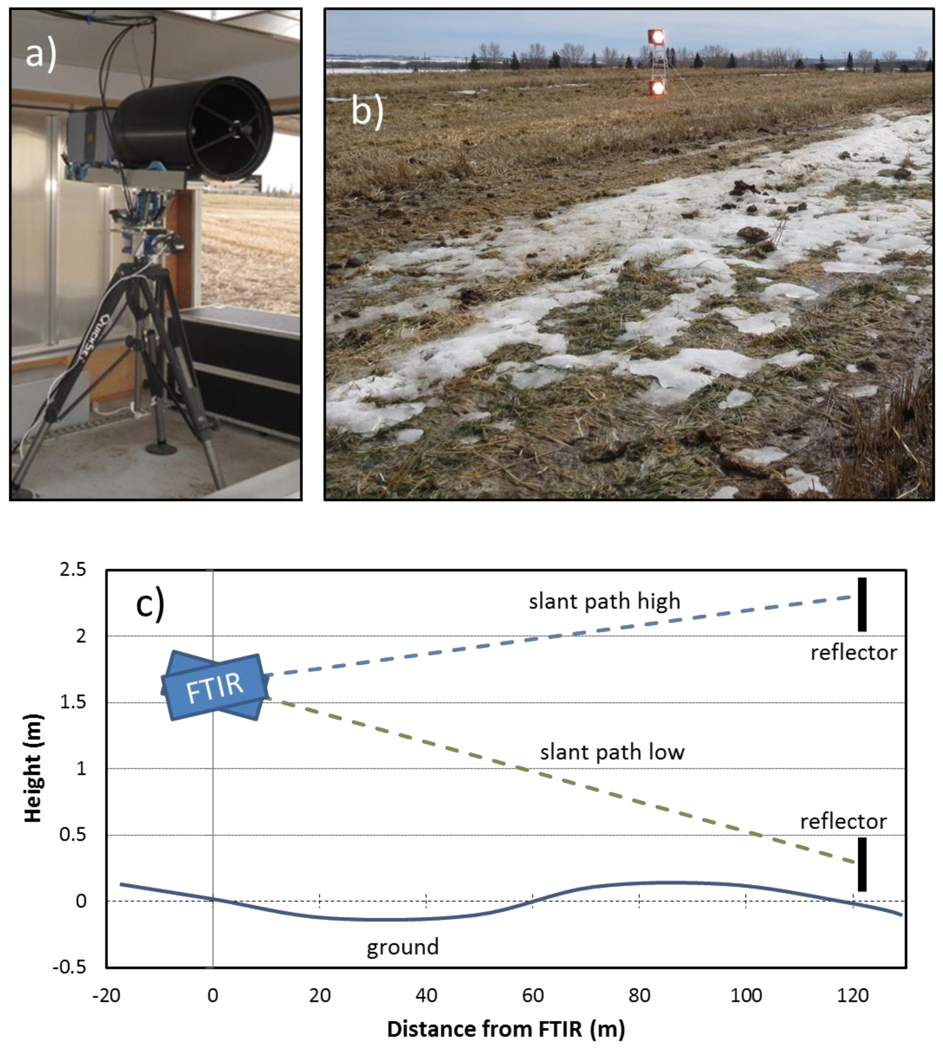
2.2. Flux Measurements
3. Results
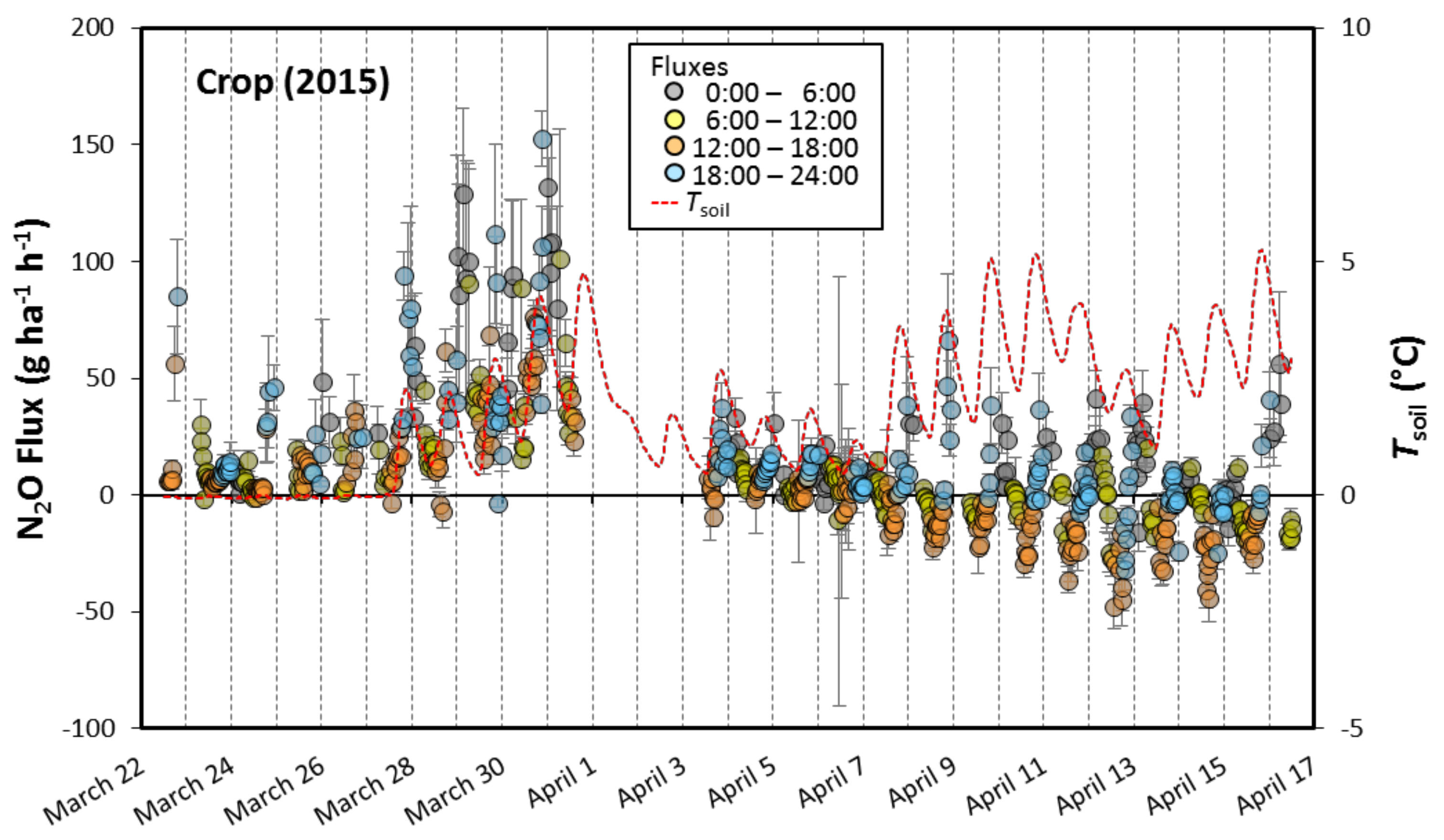
3.1. Spring Fluxes
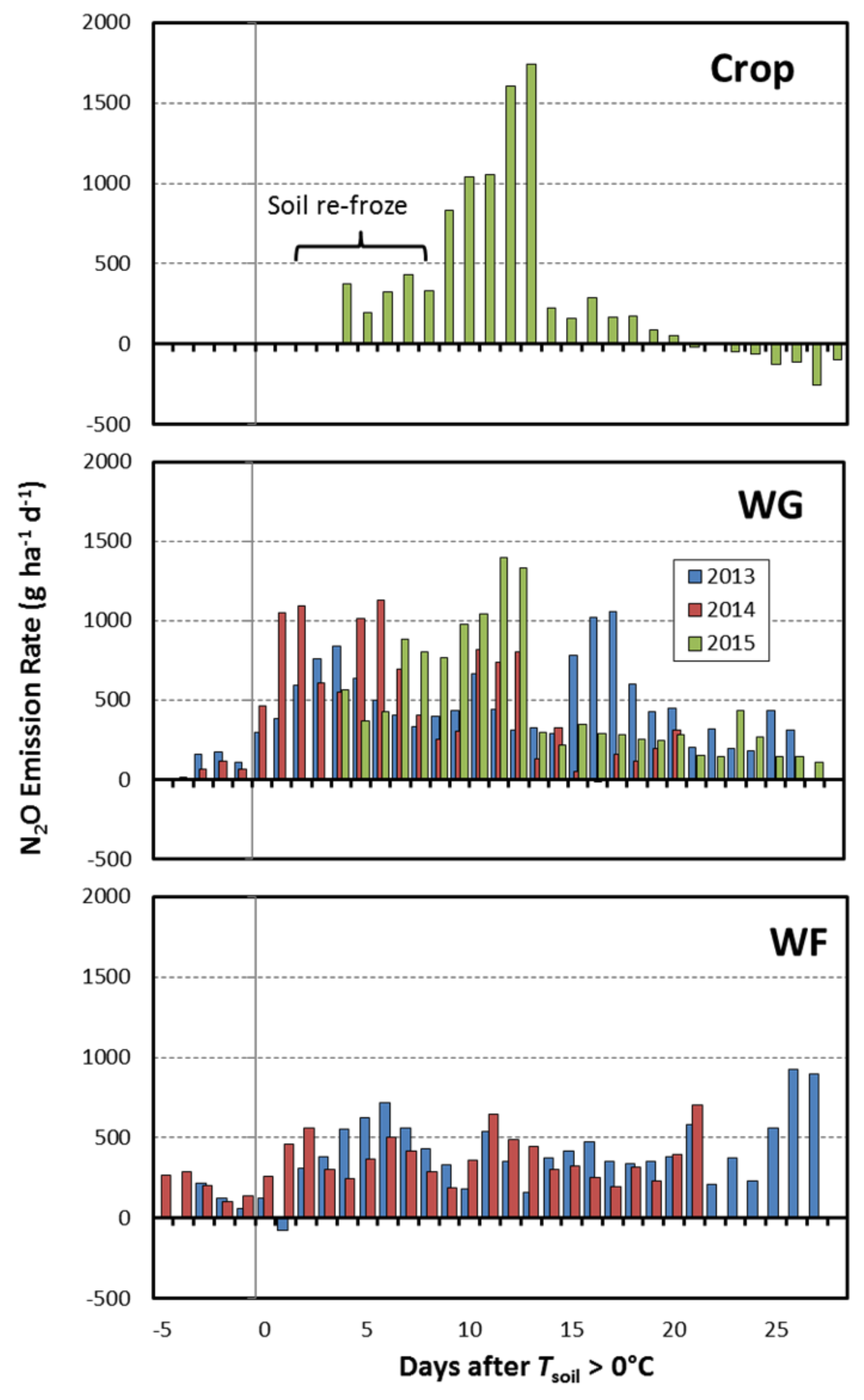
3.2. Daily Emissions
3.3. Spring N2O Losses
4. Discussion
4.1. Soil NO−3-N Levels
4.2. Other Factors
4.3. Measurement Technique
4.4. Soil Consumption
5. Conclusions
Acknowledgments
Author Contributions
Conflicts of Interest
References
- Syakila, A.; Kroeze, C. The global nitrous oxide budget revisited. Greenh. Gas Meas. Manang. 2011, 1, 17–26. [Google Scholar] [CrossRef]
- Bremner, J.M.; Robbins, S.G.; Blackmer, A.M. Seasonal variability in emission of nitrous oxide from soil. Geophys. Res. Lett. 1980, 7, 641–644. [Google Scholar] [CrossRef]
- Duxbury, J.M.; Bouldin, D.R.; Terry, R.E.; Tate III, R.L. Emissions of nitrous oxide from soils. Nature 1982, 298, 462–464. [Google Scholar] [CrossRef]
- Christensen, S.; Tiedje, J.M. Brief and vigorous N2O production by soil at springthaw. J. Soil Sci. 1990, 41, 1–4. [Google Scholar] [CrossRef]
- Wagner-Riddle, C.; Thurtell, G.W.; King, K.M.; Kidd, G.K.; Beauchamp, E.G. Nitrous oxide and carbon dioxide fluxes from a bare soil using a micrometeorological approach. J. Environ. Qual. 1997, 25, 898–907. [Google Scholar] [CrossRef]
- Lemke, R.L.; Izaurralde, R.C.; Nyborg, M. Seasonal distribution of nitrous oxide emissions from soil in the Parkland region. Soil Sci. Soc. Am. J. 1998, 62, 1320–1326. [Google Scholar] [CrossRef]
- Wagner-Riddle, C.; Congreves, K.A.; Abalos, D.; Berg, A.A.; Brown, S.E.; Ambadan, J.T.; Gao, X.; Tenuta, M. Globally important nitrous oxide emissions from croplands induced by freeze-thaw cycles. Nat. Geosci. 2017, 10, 279–283. [Google Scholar] [CrossRef]
- Nyborg, M.; Laidlaw, J.W.; Solberg, E.D.; Malhi, S.S. Denitrification and nitrous oxide emissions from a Black Chernozemic soil during spring thaw in Alberta. Can. J. Soil Sci. 1997, 77, 153–160. [Google Scholar] [CrossRef]
- Lemke, R.L.; Izaurralde, R.C.; Nyborg, M.; Solberg, E.D. Tillage and N source influence soil-emitted nitrous oxide in the Alberta Parkland region. Can. J. Soil Sci. 1999, 79, 15–24. [Google Scholar] [CrossRef]
- Izaurralde, R.C.; Lemke, R.L.; Goddard, T.W.; McConkey, B.; Zhang, Z. Nitrous oxide emissions from agricultural toposequences in Alberta and Saskatchewan. Soil Sci. Soc. Am. J. 2004, 68, 1285–1294. [Google Scholar] [CrossRef]
- Corre, M.D.; van Kessel, C.; Pennock, D.J. Landscape and seasonal patterns of nitrous oxide emissions in a semiarid region. Soil Sci. Soc. Am. J. 1996, 60, 1806–1815. [Google Scholar] [CrossRef]
- Pennock, D.J.; Corre, M.D. Development and application of landform segmentation procedures. Soil Till. Res. 2001, 58, 151–162. [Google Scholar] [CrossRef]
- Pennock, D.J.; Farrell, R.; Desjardin, R.L.; Pattey, E.; MacPherson, J.I. Upscaling chamber-based measurements of N2O emissions at snowmelt. Can. J. Soil Sci. 2005, 85, 113–125. [Google Scholar] [CrossRef]
- Environment Canada. National Inventory Report 1990–2013: Greenhouse Gas Sources and Sinks in Canada; Environment Canada: Toronto, ON, Canada, 2015. [Google Scholar]
- Chadwick, D.R.; Cardenas, L.; Misselbrook, T.H.; Smith, K.A.; Rees, R.M.; Watson, C.J.; McGeough, K.L.; Williams, J.R.; Cloy, J.M.; Thorman, R.A.; et al. Optimizing chamber methods for measuring nitrous oxide emissions from plot-based agricultural experiments. Eur. J. Soil Sci. 2014, 65, 295–307. [Google Scholar] [CrossRef]
- Grant, R.F.; Pattey, E. Mathematical modelling of nitrous oxide emissions from an agricultural field during spring thaw. Glob. Biogeochem. Cycle 1999, 13, 679–694. [Google Scholar] [CrossRef]
- Wagner-Riddle, C.; Furon, A.; McLaughlin, N.L.; Lee, I.; Barbeau, J.; Jayasundara, S.; Parkin, G.; von Bertoldi, P.; Warland, J. Intensive measurement of nitrous oxide emissions from a corn–soybean–wheat rotation under two contrasting management systems over 5 years. Glob. Chang. Biol. 2007, 13, 1722–1736. [Google Scholar] [CrossRef]
- Pattey, E.; Blackburn, L.G.; Strachan, I.B.; Desjardins, R.L.; Dow, D. Spring-thaw and growing season N2O emissions from a field planted with edible peas and a cover crop. Can. J. Soil Sci. 2008, 88, 241–249. [Google Scholar] [CrossRef]
- Glenn, A.J.; Tenuta, M.; Amiro, B.D.; Maas, S.E.; Wagner-Riddle, C. Nitrous oxide emissions from an annual crop rotation on poorly drained soil on the Canadian Prairies. Agric. For. Meteorol. 2012, 166, 41–49. [Google Scholar] [CrossRef]
- Tenuta, M.; Gao, X.; Flaten, D.N.; Amiro, B.D. Lower nitrous oxide emissions from anhydrous ammonia application prior to soil freezing in late fall than spring pre-plant application. J. Environ. Qual. 2016, 45, 1133–1143. [Google Scholar] [CrossRef] [PubMed]
- Intergovernmental Panel on Climate Change (IPCC). IPCC Guidelines for National Greenhouse Gas Inventories; Prepared by the National Greenhouse Gas Inventories Programme; IGES: Tsukuba, Japan, 2006. [Google Scholar]
- Baron, V.S.; Doce, R.R.; Basarab, J.A.; Dick, C. Swath grazing triticale and corn compared to barley and a traditional winter feeding method in central Alberta. Can. J. Plant Sci. 2014, 94, 1125–1137. [Google Scholar] [CrossRef]
- Alemu, A.W.; Doce, R.R.; Dick, A.C.; Basarab, J.A.; Kröbel, R.; Haugen-Kozyra, K.; Baron, V.S. Effect of winter feeding systems on farm greenhouse gas emissions. Agric. Syst. 2016, 148, 28–37. [Google Scholar] [CrossRef]
- National Research Council (NRC). Nutrient Requirements of Beef Cattle; The National Academies Press: Washington, DC, USA, 2000. [Google Scholar]
- Janzen, H.H.; Beauchemin, K.A.; Bruinsma, Y.; Campbell, C.; Desjardins, R.L.; Ellert, B.; Smith, E. The fate of nitrogen in agroecosystems: An illustration using Canadian estimates. Nutr. Cycl. Agroecosyst. 2003, 67, 85–102. [Google Scholar] [CrossRef]
- Etheridge, R.D.; Pesti, G.M.; Foster, E.H. A comparison of nitrogen values obtained utilizing the Kjeldahl nitrogen and Dumas combustion methodologies (Leco CNS 2000) on samples typical of an animal nutrition analytical laboratory. Anim. Feed Sci. Technol. 1998, 73, 21–28. [Google Scholar] [CrossRef]
- Flesch, T.K.; Baron, V.S.; Wilson, J.D.; Griffith, D.W.T.; Basarab, J.A.; Carlson, P.J. Agricultural gas emissions during the spring thaw: Applying a new measurement technique. Agric. For. Meteorol. 2016, 221, 111–121. [Google Scholar] [CrossRef]
- Bai, M. Methane Emissions from Livestock Measured by Novel Spectroscopic Technique. Ph.D. Thesis, University of Wollongong, Wollongong, NSW, Australia, 2010. [Google Scholar]
- Wilson, J.D.; Flesch, T.K. Generalized flux-gradient technique pairing line-average concentrations on vertically separated paths. Agric. For. Meteorol. 2016, 220, 170–176. [Google Scholar] [CrossRef][Green Version]
- Flesch, T.K.; Wilson, J.D.; Harper, L.A.; Crenna, B.P.; Sharpe, R.R. Deducing ground-air emissions from observed trace gas concentrations: A field trial. J. Appl. Meteorol. 2004, 43, 487–502. [Google Scholar] [CrossRef]
- Flesch, T.K.; McGinn, S.M.; Chen, D.; Wilson, J.D.; Desjardins, R.L. Data filtering for inverse dispersion calculations. Agric. For. Meteorol. 2015, 198–199, 1–6. [Google Scholar] [CrossRef]
- Denmead, O.T.; Freney, J.R.; Simpson, J.R. Studies of nitrous oxide emission from a grass sward. Soil Sci. Soc. Am. J. 1979, 43, 726–728. [Google Scholar] [CrossRef]
- Freibauer, A. Regionalised inventory of biogenic greenhouse gas emissions from European agriculture. Eur. J. Agron. 2003, 19, 135–160. [Google Scholar] [CrossRef]
- Shcherbak, I.; Millar, N.; Robertson, G.P. Global meta analysis of the nonlinear response of soil nitrous oxide (N2O) emissions to fertilizer nitrogen. Proc. Natl. Acad. Sci. USA 2014, 111, 9199–9204. [Google Scholar] [CrossRef] [PubMed]
- Christensen, S.; Christensen, B.T. Organic matter available for denitrification in different soil fractions: Effect of freeze/thaw cycles and straw disposal. J. Soil Sci. 1991, 42, 637–647. [Google Scholar] [CrossRef]
- Thomas, S.M.; Beare, M.H.; Francis, G.S.; Barlow, H.E.; Hedderley, D.I. Effects of tillage, simulated cattle grazing and soil moisture on N2O emissions from a winter forage crop. Plant Soil 2008, 309, 131–145. [Google Scholar] [CrossRef]
- Venterea, R.T. Theoretical comparison of advanced methods for calculating nitrous oxide fluxes using non-steady state chambers. Soil Sci. Soc. Am. J. 2013, 77, 709–720. [Google Scholar] [CrossRef]
- Ryden, J.C.; Lund, L.J.; Focht, D.D. Direct infield measurement of nitrous oxide flux from soil. Soil Sci. Soc. Am. J. 1978, 42, 731–738. [Google Scholar] [CrossRef]
- Blackmer, A.M.; Robbins, S.G.; Bremner, J.M. Diurnal variability in rate of emission of nitrous oxide from soils. Soil Sci. Soc. Am. J. 1982, 46, 937–942. [Google Scholar] [CrossRef]
- Chapuis-Lardy, L.; Wrage, N..; Metay, A.; Chotte, J.; Bernoux, M. Soils, a sink for N2O? A review. Glob. Chang. Biol. 2007, 13, 1–17. [Google Scholar] [CrossRef]
- Wen, Y.; Chen, Z.; Dannenmann, M.; Carminati, A.; Willibald, G.; Kiese, R.; Wolf, B.; Veldkamp, E.; Butterbacn-Bahl, K.; Corre, M.D. Disentangling gross N2O production and consumption in soil. Sci. Rep. 2016, 6, 36517. [Google Scholar] [CrossRef] [PubMed]


| 2012–2013 | 2013–2014 | 2014–2015 | ||||
|---|---|---|---|---|---|---|
| Winter-Feeding | Winter-Grazing | Winter-Feeding | Winter-Grazing | Crop | Winter-Grazing | |
| Area of site (ha) | 2.6 | 2.5 | 2.6 | 2.5 | 2.5 | 2.5 |
| Crop | - | corn | - | triticale | triticale | triticale |
| Cattle-days a (ha−1) | 1346 | 1446 | 2894 | 459 | 0 | 1063 |
| Cattle feed | barley-silage, straw | swathed corn | barley-silage, straw | swathed triticale | - | swathed triticale |
| N Inputs (kg ha−1): | ||||||
| fertilizer b | - | 55 | - | 92 | 55 | 55 |
| manure c | 217 | 181 | 593 | 72 | - | 117 |
| roots + residue d | - | 82 | - | 172 | 56 | 118 |
| mineralization e | - | - | - | - | 60 | - |
| NH3 deposition f | 5 | 5 | 5 | 5 | 5 | 5 |
| Total | 222 | 323 | 598 | 341 | 176 | 295 |
| Soil test g (µg g−1) | ||||||
| NO3-N | NA | 35 | NA | 58 | 57 | 28 |
| NH4-N | NA | 5.4 | NA | 5.4 | 7.0 | 7.1 |
| 2012–2013 | 2013–2014 | 2014–2015 | ||||
| Precipitation (Sep.–Apr.) | 133 mm | 173 mm | 162 mm | |||
| Soil freeze/thaw: 5 cm | 11 Nov./1 Apr. | 7 Dec./9 Apr. | 14 Nov./18 Mar. | |||
| CFD h | 432 | 317 | 339 | |||
| Crop | Winter-Feeding | Winter-Grazing | ||||
|---|---|---|---|---|---|---|
| 2015 | 2013 | 2014 | 2013 | 2014 | 2015 | |
| N2O Measurements (kg N2O-N ha−1) | ||||||
| 2O-N loss (# days) | 5.3 (25) | 7.7 (31) | 6.3 (29) | 8.9 (31) | 7.3 (29) | 7.7 (25) |
| N2O-N Loss Estimates | ||||||
| IPCC: annual loss a | 1.8 | 4.4 | 11.9 | 5.0 | 4.1 | 4.1 |
| NIR: annual loss b | 1.1 | 0.1 | 0.3 | 3.1 | 3.2 | 2.8 |
| Freibauer: annual loss c | 17.9 | 11.3 | 17.8 | 9.8 | ||
© 2018 by the authors. Licensee MDPI, Basel, Switzerland. This article is an open access article distributed under the terms and conditions of the Creative Commons Attribution (CC BY) license (http://creativecommons.org/licenses/by/4.0/).
Share and Cite
Flesch, T.K.; Baron, V.S.; Wilson, J.D.; Basarab, J.A.; Desjardins, R.L.; Worth, D.; Lemke, R.L. Micrometeorological Measurements Reveal Large Nitrous Oxide Losses during Spring Thaw in Alberta. Atmosphere 2018, 9, 128. https://doi.org/10.3390/atmos9040128
Flesch TK, Baron VS, Wilson JD, Basarab JA, Desjardins RL, Worth D, Lemke RL. Micrometeorological Measurements Reveal Large Nitrous Oxide Losses during Spring Thaw in Alberta. Atmosphere. 2018; 9(4):128. https://doi.org/10.3390/atmos9040128
Chicago/Turabian StyleFlesch, Thomas K., Vern S. Baron, John D. Wilson, John A. Basarab, Raymond L. Desjardins, Devon Worth, and Reynald L. Lemke. 2018. "Micrometeorological Measurements Reveal Large Nitrous Oxide Losses during Spring Thaw in Alberta" Atmosphere 9, no. 4: 128. https://doi.org/10.3390/atmos9040128
APA StyleFlesch, T. K., Baron, V. S., Wilson, J. D., Basarab, J. A., Desjardins, R. L., Worth, D., & Lemke, R. L. (2018). Micrometeorological Measurements Reveal Large Nitrous Oxide Losses during Spring Thaw in Alberta. Atmosphere, 9(4), 128. https://doi.org/10.3390/atmos9040128