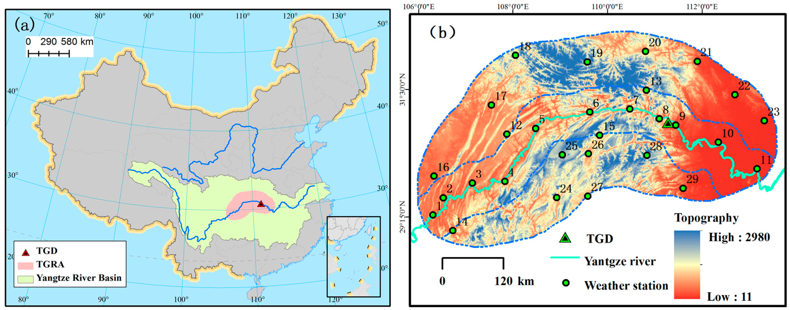
Figure 1.
Location of the Three Gorges Reservoir area (
a); the topography of Three Gorges Reservoir area and the location of weather stations (
b). Further weather station information is provided in supplemental
Table 1.
Figure 1.
Location of the Three Gorges Reservoir area (
a); the topography of Three Gorges Reservoir area and the location of weather stations (
b). Further weather station information is provided in supplemental
Table 1.
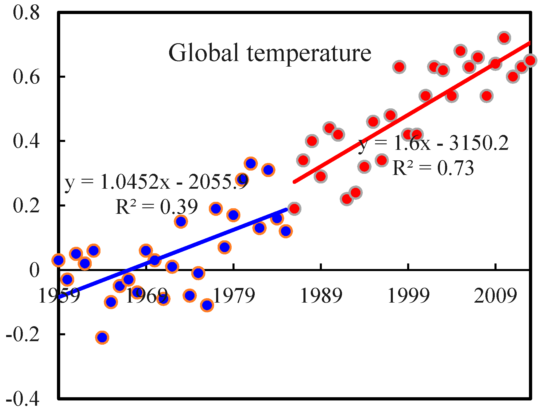
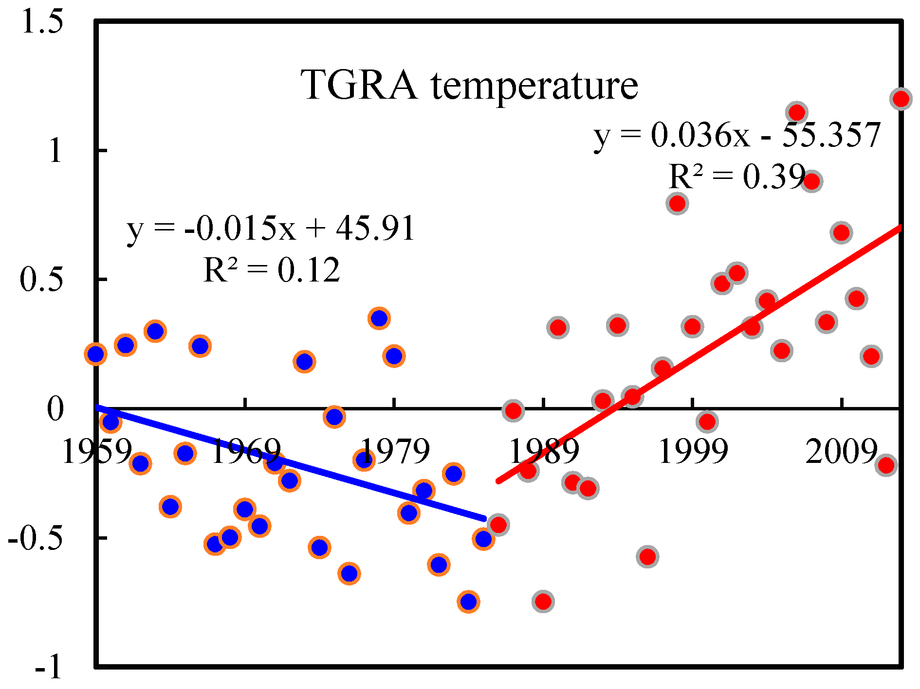
Figure 2.
Global and TGRA air temperature changes for the period 1959 to 2013.
Figure 2.
Global and TGRA air temperature changes for the period 1959 to 2013.
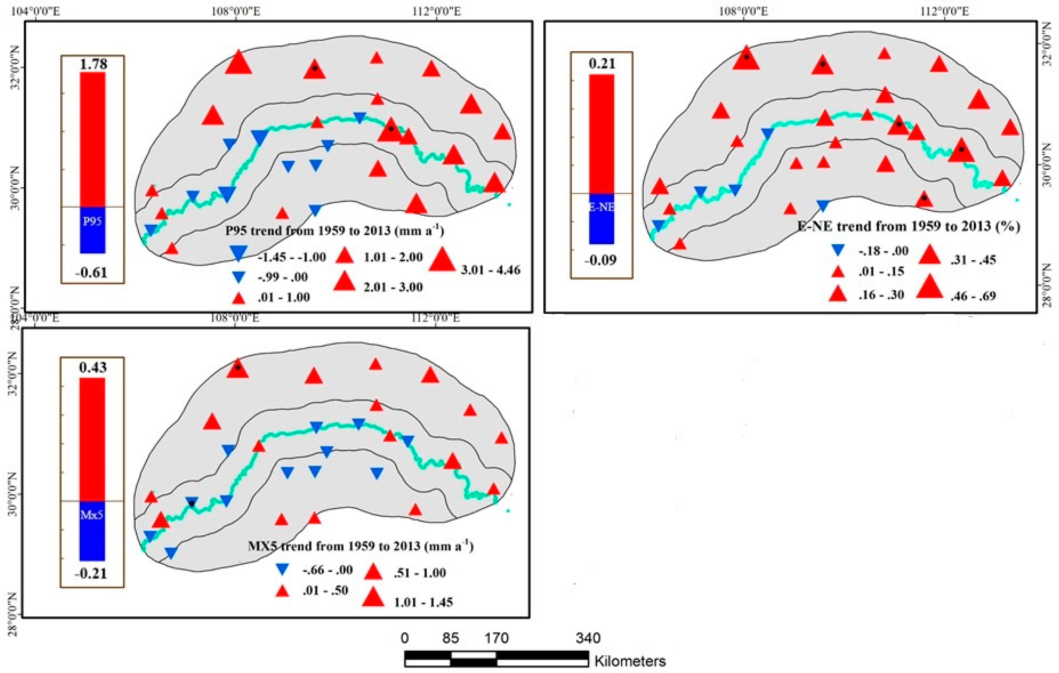
Figure 3.
Changes in P95, (E–NE, Mx5 for the period of 1959–2013. Red upward and blue downward triangles indicate increasing and decreasing tendencies, respectively. The triangle size represents the magnitude of these positive and negative trends. The black spot in the triangles represents significant trends at a 5% significance level. The red bar is the median slope of upward trend stations, while the blue bar is the median slope of downward trend stations.
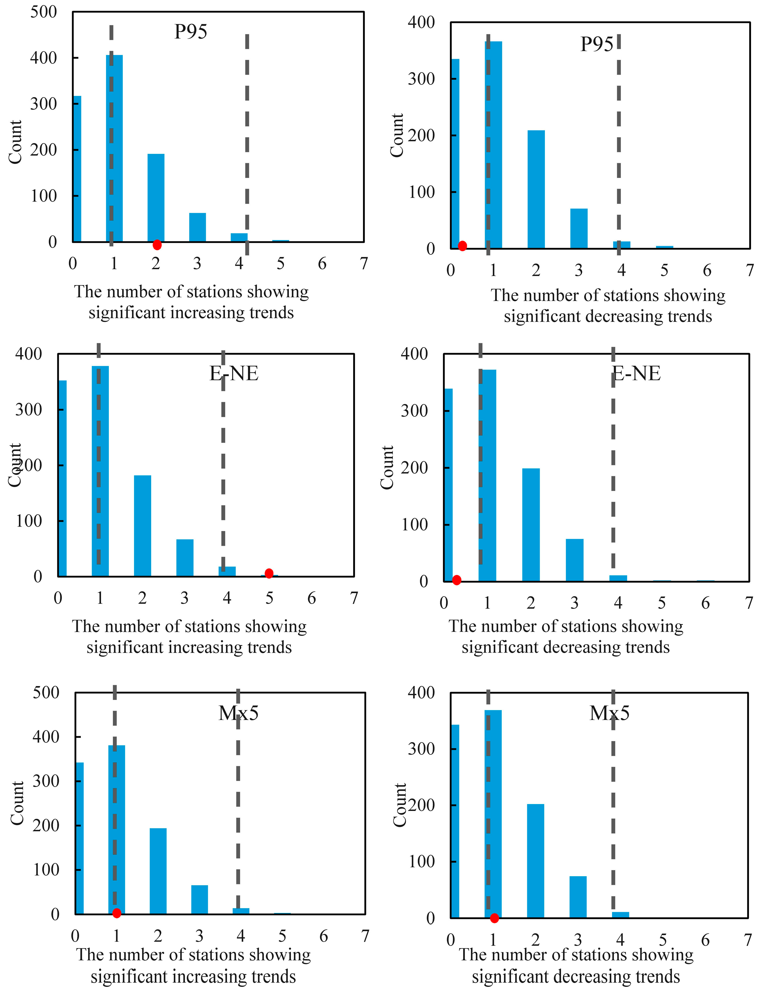
Figure 4.
The field significant test for statistically significant increasing and decreasing trends. The bar chart represents the distribution of stations with a statistically significant trend after implementing the MK (Mann–Kendall) test on 1000 bootstrap extreme precipitation indices. The area between vertical black dashed lines represents 95% of the distribution. The red filled circle represents the number of stations with a statistically significant trend.
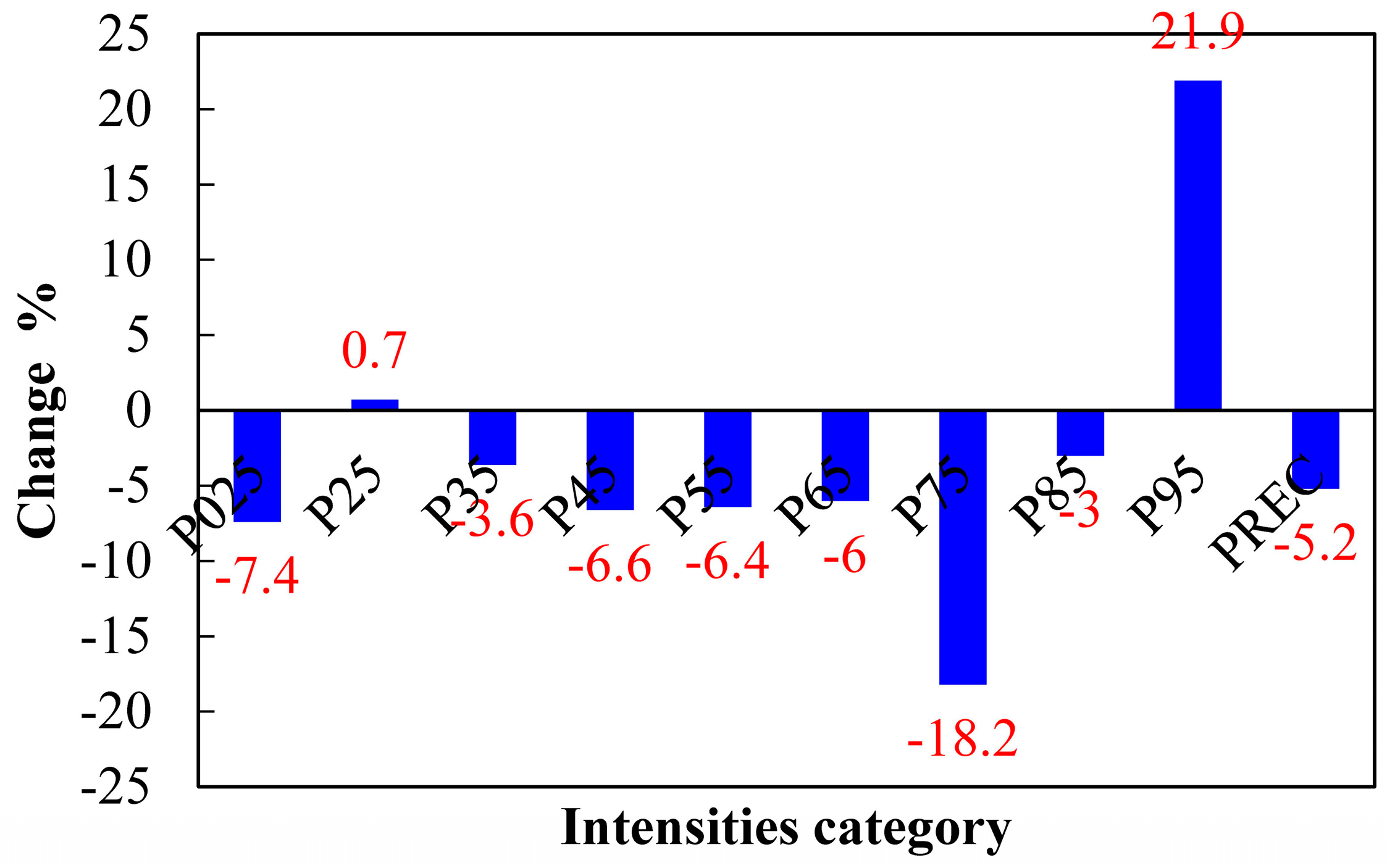
Figure 5.
Median changes (%) of precipitation amount for nine precipitation intensities among 29 stations during the period of 1959–2013.
Figure 5.
Median changes (%) of precipitation amount for nine precipitation intensities among 29 stations during the period of 1959–2013.
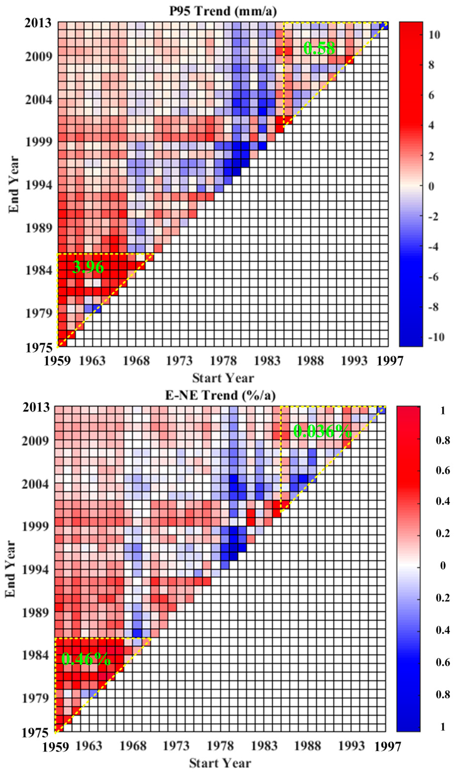
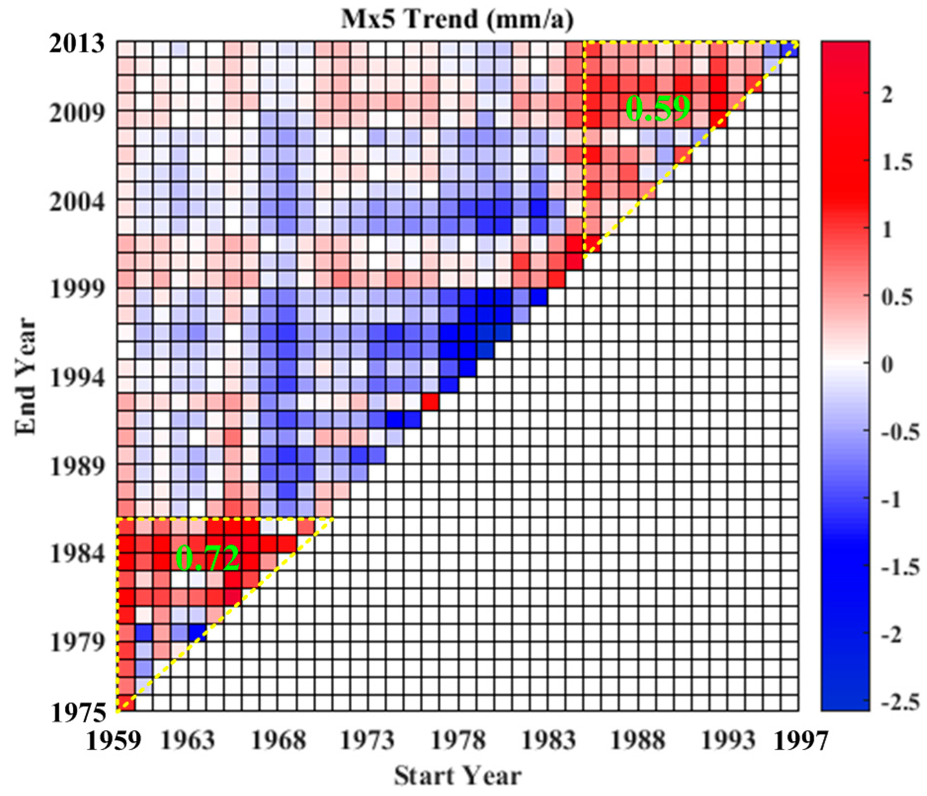
Figure 6.
Median Sen’s slopes in P95, E–NE and Mx5 among 29 stations during different time spans for periods with different starting years (1959–1997) and ending years (1975–2013). Median Sen’s slopes within the downward yellow triangle were from 1959 to 1985, while median Sen’s slopes within the upward yellow triangle were from 1986 to 2013. (/a = per annual).
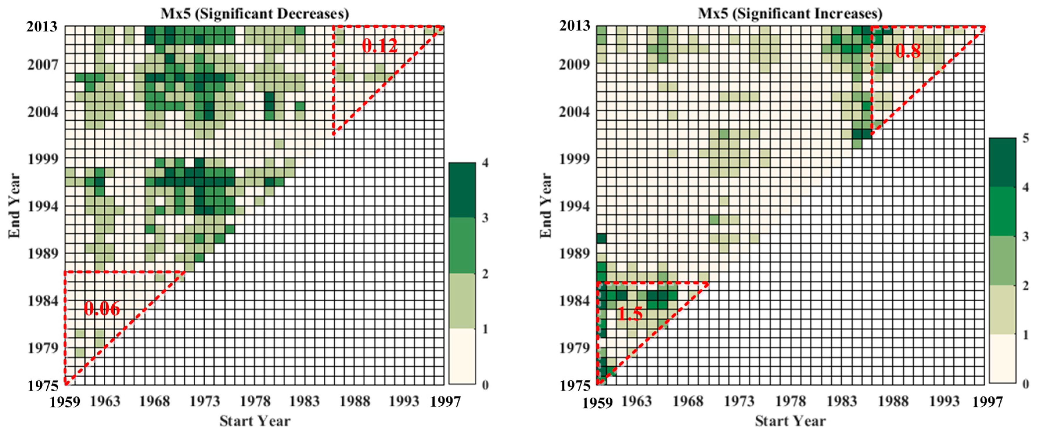
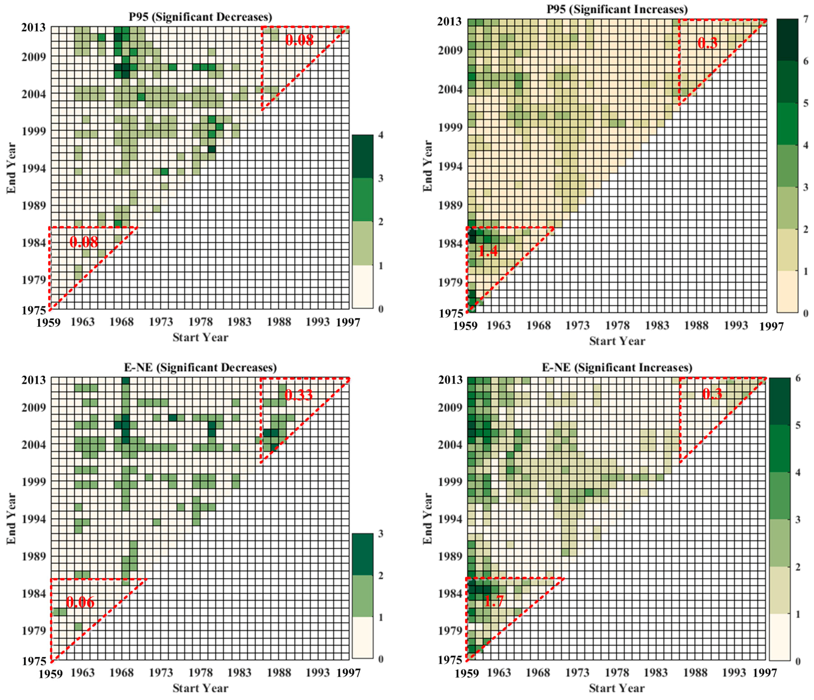
Figure 7.
Number of stations with significant decreasing (left panel) and increasing (right panel) trends in P95, E–NE and Mx5 during different time spans for periods with different starting years (1959–1997) and ending years (1975–2013). Number of stations within downward red triangles were from 1959 to 1985, while number of stations within upward red triangles were from 1986 to 2013.
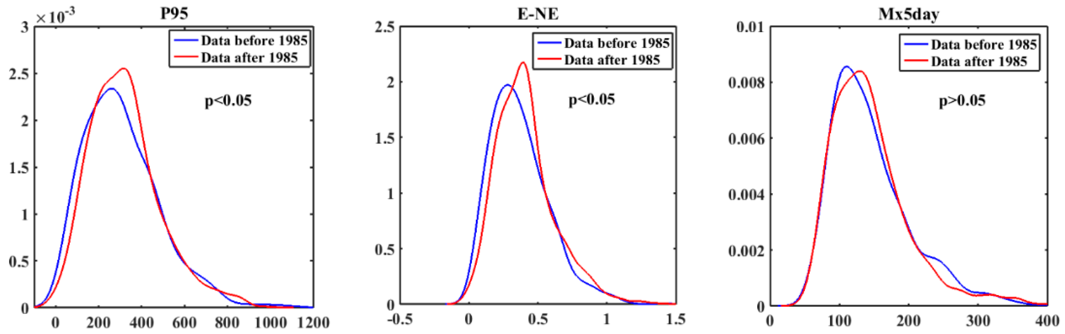
Figure 8.
Density distributions for P95, E-NE and Mx5, respectively, for the pre-1985 (blue) and post-1985 (red) periods. Statistical significance was estimated using the Kolmogorov–Smirnov test for distributions of the extreme precipitation indices.
Figure 8.
Density distributions for P95, E-NE and Mx5, respectively, for the pre-1985 (blue) and post-1985 (red) periods. Statistical significance was estimated using the Kolmogorov–Smirnov test for distributions of the extreme precipitation indices.
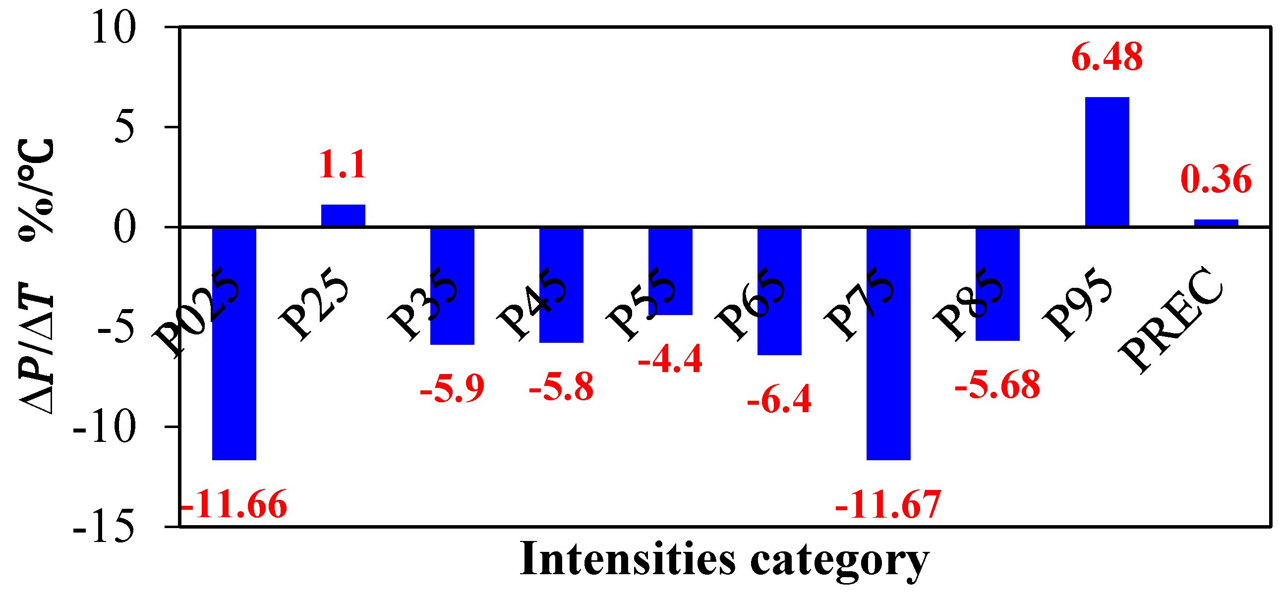
Figure 9.
Changes in precipitation amount for nine precipitation intensities and PREC per one-degree Celsius increase in global surface temperature (%/°C).
Figure 9.
Changes in precipitation amount for nine precipitation intensities and PREC per one-degree Celsius increase in global surface temperature (%/°C).
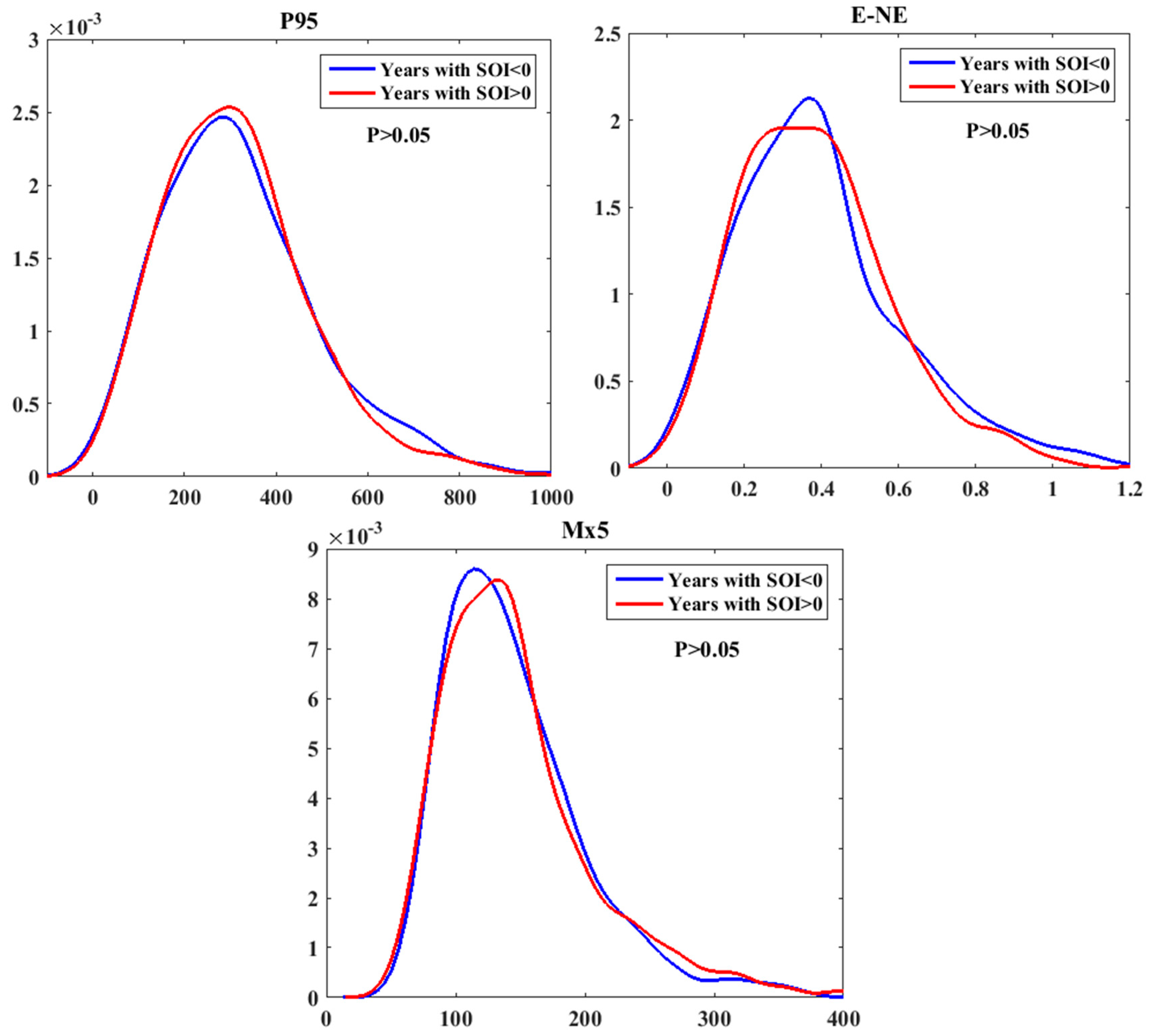
Figure 10.
Density distributions for P95, E-NE and Mx5, respectively, for the class I years (blue) and class II years (red) periods. Statistical significance was estimated using the Kolmogorov–Smirnov test for distributions of the extreme precipitation indices.
Figure 10.
Density distributions for P95, E-NE and Mx5, respectively, for the class I years (blue) and class II years (red) periods. Statistical significance was estimated using the Kolmogorov–Smirnov test for distributions of the extreme precipitation indices.
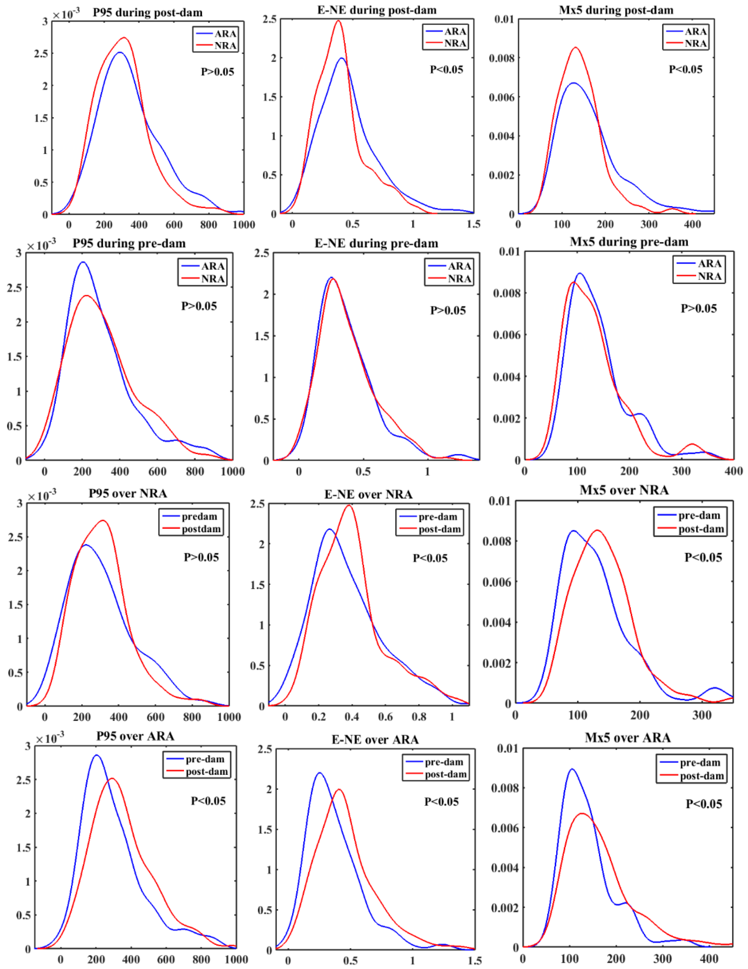
Figure 11.
Density distributions for P95, E–NE and Mx5, respectively, for the pre- and post- dam periods, over the ARA (reservoir area) and the NRA (near reservoir area). Statistical significance was estimated using the Kolmogorov–Smirnov test for distributions of the extreme precipitation indices.
Figure 11.
Density distributions for P95, E–NE and Mx5, respectively, for the pre- and post- dam periods, over the ARA (reservoir area) and the NRA (near reservoir area). Statistical significance was estimated using the Kolmogorov–Smirnov test for distributions of the extreme precipitation indices.
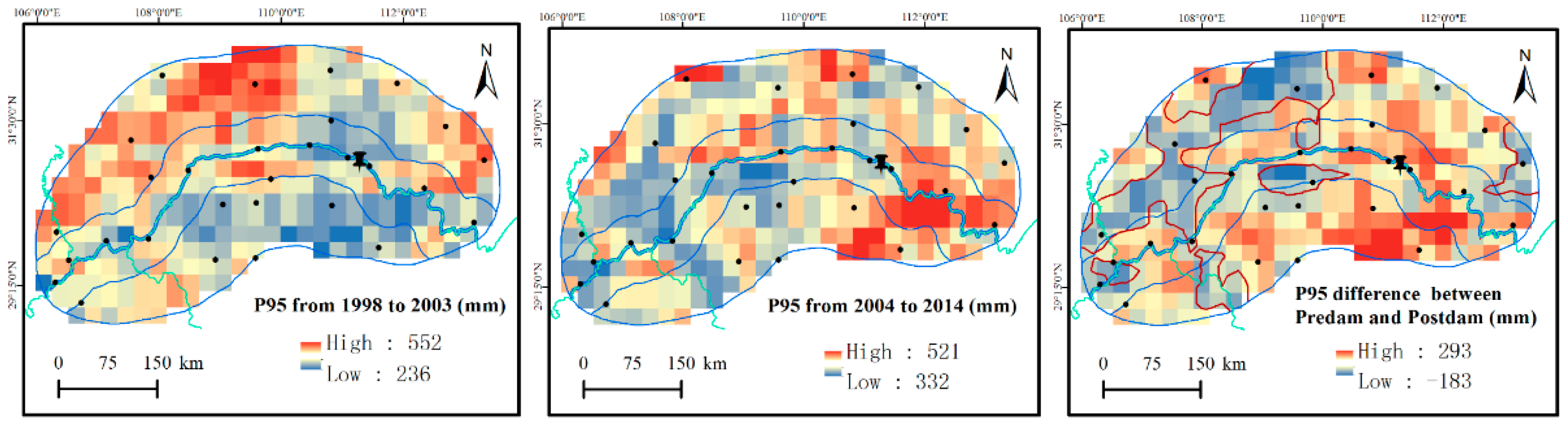
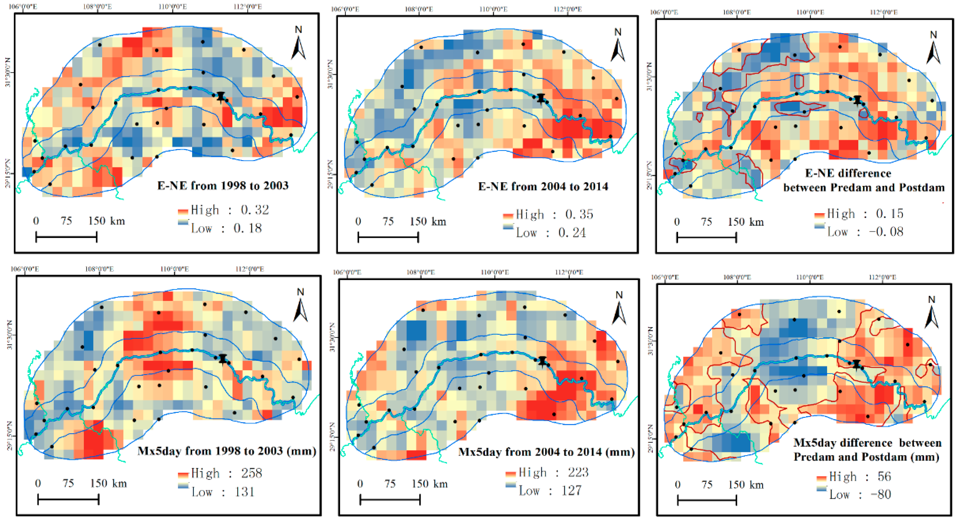
Figure 12.
Spatial distribution of mean P95, E–NE, Mx5 from TRMM data for pre-dam and post-dam period, their difference between pre-dam and post-dam period.
Figure 12.
Spatial distribution of mean P95, E–NE, Mx5 from TRMM data for pre-dam and post-dam period, their difference between pre-dam and post-dam period.
Table 1.
Extreme climate indices used in this study.
Table 1.
Extreme climate indices used in this study.
| Code | Indicator Name | Definition | Units |
|---|
| Mx5 | Maximum 5-day precipitation amount | Annual maximum consecutive 5-day precipitation | mm |
| P95 | Heavy precipitation | Annual precipitation amount when daily rainfall >95th percentile | mm |
| E-NE | Extreme precipitation to non-extreme precipitation ratio | P95/(Annual total precipitation—P95).
E–NE is the ratio of annual extreme precipitation (P95) to annual non-extreme precipitation. Extreme precipitation is the sum of extreme rainfall events exceeding the 95th percentile for each year, while non-extreme rainfall is estimated after subtracting heavy rainfall from the annual rainfall total. | Fraction |
| P025 | Light precipitation | Annual precipitation amount when daily rainfall <25th percentile | mm |
| P25 | Light precipitation | Annual precipitation amount when daily rainfall is between the 25th percentile and 35th percentile | mm |
| P35 | Light precipitation | Annual precipitation amount when daily rainfall is between the 35th percentile and 45th percentile | mm |
| P45 | Light precipitation | Annual precipitation amount when daily rainfall is between the 45th percentile and 55th percentile | mm |
| P55 | Middle precipitation | Annual precipitation amount when daily rainfall is between the 55th percentile and 65th percentile | mm |
| P65 | Middle precipitation | Annual precipitation amount when daily rainfall is between the 65th percentile and 75th percentile | mm |
| P75 | Middle precipitation | Annual precipitation amount when daily rainfall is between the 75th percentile and 85th percentile | mm |
| P85 | Middle precipitation | Annual precipitation amount when daily rainfall is between the 85th percentile and 95th percentile | mm |
| PREC | Annual precipitation | Annual precipitation | mm |
Table 2.
Abrupt change year of air temperature at 29 stations.
Table 2.
Abrupt change year of air temperature at 29 stations.
| No. | Name | Change Point Year | Trend test | No. | Name | Change Point Year | Trend Test |
|---|
| From 1959 to Change Point Year | From Change Point Year to 2013 | From 1959 to 2013 | From 1959 to Change Point Year | From Change Point to Year 2013 | From 1959 to 2013 |
|---|
| 1 | Jiangjing | 1989 | − | + | + | 16 | Hechuan | 1996 | − | + | + |
| 2 | Shapingba | 1985 | − | + | + | 17 | Daxian | 1987 | − | + | + |
| 3 | Changshou | 1983 | − | + | + | 18 | Wanyuan | 1996 | − | + | + |
| 4 | Fengdu | 1996 | − | + | + | 19 | Zhengping | 1983 | − | + | + |
| 5 | Wanzhou | 1985 | − | + | + | 20 | Fangxian | 1987 | − | + | – |
| 6 | Fengjie | 1983 | − | + | + | 21 | Nanzhang | 1983 | − | + | + |
| 7 | Badong | 1993 | + | – | − | 22 | Zhongxiang | 1987 | − | + | + |
| 8 | Zigui | 1985 | − | + | + | 23 | Tianmen | 1983 | − | + | + |
| 9 | Yichang | 1986 | − | + | + | 24 | Qianjiang | 1985 | − | + | + |
| 10 | Jingzhou | Ns | / | / | + | 25 | Lichuan | 1983 | − | + | + |
| 11 | Jianli | 1993 | − | + | + | 26 | Enshi | 1985 | − | + | + |
| 12 | Liangping | 1985 | − | + | + | 27 | Laifeng | 1983 | − | + | + |
| 13 | Xingshan | 1986 | − | + | + | 28 | Wufeng | Ns | / | / | + |
| 14 | Qijiang | 1985 | − | + | + | 29 | Shimen | 1985 | − | + | + |
| 15 | Jianshi | 1986 | − | + | + | | | | | | |
Table 3.
Statistical difference tests in the mean in the extreme rainfall indices (P95/mm, E–NE (fraction) and MX5/mm) between pre-1985 and post-1985 periods.
Table 3.
Statistical difference tests in the mean in the extreme rainfall indices (P95/mm, E–NE (fraction) and MX5/mm) between pre-1985 and post-1985 periods.
| Extreme Indices | Pre-1985 | Post-1985 | p-mw |
|---|
| P95 | 308.64 | 321.95 | <0.05 |
| E-NE | 0.37 | 0.41 | <0.01 |
| Mx5 | 145.74 | 145.32 | 0.94 |
Table 4.
Statistical difference tests for the mean and distribution in the RH (%) and WP (hPa) between pre-1985 and post-1985 periods.
Table 4.
Statistical difference tests for the mean and distribution in the RH (%) and WP (hPa) between pre-1985 and post-1985 periods.
| Indices | Pre-1985 | Post-1985 | p-mw | p-ks |
|---|
| RH | 78.6 | 77.4 | <0.01 | <0.01 |
| WP | 5.45 | 5.33 | <0.05 | <0.01 |
Table 5.
Statistical difference tests for the mean in the extreme rainfall indices (P95/mm, E–NE (fraction), MX5/mm) in between class I years with SOI < 0 and class II years with SOI > 0.
Table 5.
Statistical difference tests for the mean in the extreme rainfall indices (P95/mm, E–NE (fraction), MX5/mm) in between class I years with SOI < 0 and class II years with SOI > 0.
| Extreme Indices | SOI < 0 | SOI > 0 | p-mw |
|---|
| P95 | 321.9 | 312.7 | 0.57 |
| E-NE | 0.398 | 0.385 | 0.63 |
| Mx5 | 145.9 | 147.4 | 0.82 |
Table 6.
Statistical difference tests for the mean in the extreme rainfall indices (P95/mm, E–NE (fraction) and Mx5/mm) from weather stations for the different periods. (ARA: reservoir area and the NRA: near reservoir area).
Table 6.
Statistical difference tests for the mean in the extreme rainfall indices (P95/mm, E–NE (fraction) and Mx5/mm) from weather stations for the different periods. (ARA: reservoir area and the NRA: near reservoir area).
| Paired Analysis | Precipitation Indices | Location | Periods | p-mw |
|---|
| Pre-Dam | Post-Dam |
|---|
| 1 | P95 | NRA | 305.02 | 308.29 | 0.45 |
| E-NE | NRA | 0.37 | 0.40 | 0.18 |
| Mx5 | NRA | 131.11 | 141.2 | <0.05 |
| 2 | P95 | ARA | 296.64 | 348.89 | <0.01 |
| E-NE | ARA | 0.368 | 0.46 | <0.01 |
| Mx5 | ARA | 138.36 | 164.78 | <0.01 |
Table 7.
Statistical difference tests for the mean in the extreme rainfall indices (P95/mm, E–NE (fraction) and Mx5/mm) from weather stations for the different locations.
Table 7.
Statistical difference tests for the mean in the extreme rainfall indices (P95/mm, E–NE (fraction) and Mx5/mm) from weather stations for the different locations.
| Paired Analysis | Precipitation Indices | Period | Locations | p-mw |
|---|
| NAR | ARA |
|---|
| 3 | P95 | Post-dam | 348.9 | 308.29 | <0.05 |
| E-NE | Post-dam | 0.46 | 0.40 | <0.01 |
| Mx5 | Post-dam | 164.78 | 141.2 | <0.01 |
| 4 | P95 | Pre-dam | 296.64 | 305.02 | 0.54 |
| E-NE | Pre-dam | 0.37 | 0.37 | 0.68 |
| Mx5 | Pre-dam | 138.36 | 131.11 | 0.10 |
Table 8.
Statistical difference tests for the mean and distribution in the extreme rainfall indices (P95/mm, E–NE (fraction) and Mx5/mm) from TRMM data for the different periods.
Table 8.
Statistical difference tests for the mean and distribution in the extreme rainfall indices (P95/mm, E–NE (fraction) and Mx5/mm) from TRMM data for the different periods.
| Paired Analysis | Precipitation Indices | Location | Periods | p-mw | p-ks |
|---|
| Pre-Dam | Post-Dam |
|---|
| 1 | P95 | NRA | 265 | 411 | <0.01 | <0.01 |
| E-NE | NRA | 0.18 | 0.29 | <0.01 | <0.01 |
| Mx5 | NRA | 133 | 167 | <0.01 | <0.01 |
| 2 | P95 | ARA | 355 | 405 | <0.01 | <0.01 |
| E-NE | ARA | 0.24 | 0.28 | <0.01 | <0.01 |
| Mx5 | ARA | 163 | 166 | 0.85 | <0.01 |
Table 9.
Statistical difference tests for the mean and distribution in the extreme rainfall indices (P95/mm, E–NE (fraction) and Mx5/mm) from TRMM data for the different locations.
Table 9.
Statistical difference tests for the mean and distribution in the extreme rainfall indices (P95/mm, E–NE (fraction) and Mx5/mm) from TRMM data for the different locations.
| Paired Analysis | Precipitation Indices | Period | Locations | p-mw | p-ks |
|---|
| ARA | NRA |
|---|
| 3 | P95 | Post-dam | 405 | 411 | 0.54 | 0.57 |
| E-NE | Post-dam | 0.28 | 0.29 | 0.10 | 0.18 |
| Mx5 | Post-dam | 166 | 167 | 0.37 | 0.14 |
Table 10.
Statistical difference tests for the mean and distribution in the RH (%) and WP (hPa) at the same locations for the different periods.
Table 10.
Statistical difference tests for the mean and distribution in the RH (%) and WP (hPa) at the same locations for the different periods.
| Paired Analysis | Precipitation Indices | Location | Periods | p-mw | p-ks |
|---|
| Pre-Dam | Post-Dam |
|---|
| 1 | WP | NRA | 5.38 | 5.22 | <0.01 | <0.01 |
| RH | NRA | 77.6 | 75.1 | <0.01 | <0.01 |
| 2 | WP | ARA | 5.38 | 5.26 | <0.01 | <0.01 |
| RH | ARA | 78.6 | 76.7 | <0.01 | <0.01 |
Table 11.
Statistical difference tests for the mean and distribution in the RH (%) and WP (hPa) at the same locations for the different locations.
Table 11.
Statistical difference tests for the mean and distribution in the RH (%) and WP (hPa) at the same locations for the different locations.
| Paired Analysis | Precipitation Indices | Period | Locations | p-mw | p-ks |
|---|
| NAR | ARA |
|---|
| 3 | WP | Post-dam | 5.22 | 5.26 | 0.56 | 0.35 |
| RH | Post-dam | 75.1 | 76.7 | <0.01 | <0.01 |
| 4 | WP | Pre-dam | 5.38 | 5.38 | 0.5 | <0.01 |
| RH | Pre-dam | 77.6 | 78.6 | 0.13 | 0.14 |


