Abstract
This sensitivity study examined the impact of drizzle on hailstorm characteristics and precipitation on the ground. A cloud-resolving mesoscale model with a two-moment bulk microphysical scheme is modified by introducing mixing ratio and number concentration of drizzle. Therefore, the cloud model integrates the mixing ratio and number concentration of the eight microphysical particles: cloud droplets, drizzle, raindrops, cloud ice, snowflakes, graupel, frozen raindrops and hailstones. We compared two microphysical schemes depending on whether drizzle particles are present or not. It can be noted that the presence of drizzle category slows the development of the rain in the hailstorm and its appearance on the ground. The increased values of radar reflectivity factor in simulations with drizzle are a result of significantly higher values of raindrop number concentration rather than their sizes and indicate the presence of hail as well. There are prominent decreases of the radar reflectivity factor in simulations with drizzle. The occurrence of heavy showers does not exist in results without drizzle. The absence of drizzle category leads to greater accumulations of rain and a wider area of downdrafts. The alternate case produces both weaker downdrafts and smaller area of downdraft cells due to a slower autoconversion of drizzle to rain and a smaller rain evaporation. A smaller amount of surface hail is expected in the non-drizzle case.
1. Introduction
Cumulonimbus clouds contribute significantly to the total rainfall on the Earth. They play an important role in both global atmospheric circulation and maintenance of the static fair-weather electric field due to their permanent presence in equatorial latitudes. Additionally, they often produce electric discharges, large hailstones, heavy rainfall, flash floods, wind gusts and tornadoes. These phenomena may result in loss of property and human life. Therefore, in addition to theoretical considerations, investigation of cumulonimbus clouds in preventing or minimizing possible damage using numerical models is of great importance.
Cloud-resolving mesoscale models are a powerful practical tool for exploring the inner structure of clouds and forecasting of cloud motion and the amounts of surface precipitation generated by clouds. These numerical models use explicit bin [1,2] or bulk microphysical schemes [3,4,5,6,7]. The bulk microphysical scheme uses a size distribution function for microphysical particles which is represented by one or more corresponding moments (e.g., mixing ratio, number concentration, radar reflectivity).
So far, the impact of raindrop embryos is not considered in numerical studies of hailstorms using the bulk microphysical scheme. The models only use two categories of water drops: non-precipitating/cloud droplets and precipitating drops/raindrops. In these numerical models, cloud droplets are transformed to raindrops via an autoconversion process either immediately [8,9] or when cloud water mixing ratio reached a certain constant value [10,11]. In the literature, there is no representation of the transition part of the spectrum between categories of cloud droplets and raindrops. Therefore, there is no description of small precipitation drops that are small enough to reach the ground rarely (due to their evaporation and collection with other precipitating elements—raindrops, hailstone embryos and hail) and at the same time large enough that they cannot be treated as cloud droplets. These raindrop embryos can be identified as drizzle.
Drizzle particles are water drops with a diameter between 0.2 and 0.5 mm [12]. They are the precipitating particles usually associated with stratiform clouds–stratus and stratocumulus [13,14,15]. In the literature, there are numerous numerical and observational studies about drizzle particles. However, these studies consider a drizzle presence in stratus and stratocumulus clouds [16,17,18,19,20,21] and cumulus ones [22,23,24] and until now not as a separate category in hailstorms. From observations of small cumuli, Hudson and Yum (2001) [22] concluded that the presence of a drizzle is much greater in maritime clouds than continental ones. Higher CCN concentrations in continental clouds lead to drizzle suppression. In a modeling study of small cumulus, Gerber and Frick (2012) [24] concluded that the drizzle rate is affected by large sea-salt nuclei and increases as wind speed increases. At constant wind speeds, the drizzle rate decreases with increasing in-cloud droplet concentration.
However, a lack of observational studies about the drizzle precipitation from hailstorms does not mean that they cannot exist in the clouds and have no influence on the development of other cloud and precipitating particles, especially raindrops. Whereas raindrops usually have diameters approximately 1–2 mm [12], drizzle can be identified as initial, embryonic raindrops. Gilmore and Straka (2008) [25] concluded that drizzle should be presented as a separate category of drops to avoid the use of a unimodal size distribution for drizzle and raindrops. We assume that drizzle is formed in the same manner as rain (in the bulk microphysical scheme without drizzle) by the autoconversion of cloud droplets (collision–coalescence process). Therefore, mutual collision and coalescence of cloud droplets should rather create either larger cloud droplets or droplets with size that can be recognized as drizzle in the bulk microphysical scheme. The gradual development of the liquid phase in numerical models of hailstorm can prevent the early presence of rain in cloud and its rapid detection on the ground after only a few minutes from the beginning of the simulation, as reported in some numerical studies [7]. Further, the existence of a size subcategory of small water drops contributes to discovering of riming process in more detail.
In this preliminary study, we focused on the impact of the presence of drizzle category on surface precipitation and microphysical and dynamical characteristics of hailstorms. In our experiment, we upgraded the model which uses a unified Khrgian–Mazin size distribution for two drop categories [26,27] to the one with three categories, by including drizzle category between cloud droplets and raindrops, i.e., drizzle particles cover the range of diameters which was related to the lower part of rain size distribution in the version of the model without drizzle. We use this representation of drop size spectrum to avoid the unnatural gaps at the size boundaries among drop categories. In this way we inspect the impact of drizzle particles as a separate category on the hailstorm in the bulk microphysical scheme. Appropriate size boundaries among the certain category of drops we defined by following Glickman (2000) [12].
2. Model Description
2.1. General Model Features
The model of hailstorms [7,27,28] was modified with the mass and number concentration of drizzle particles as prognostic variables. Additionally, aerosol particles are explicitly represented in the model. The numerical model calculates time-dependent, non-hydrostatic and fully compressible equations. The prognostic variables of the model are the three Cartesian wind components: perturbation potential temperature, perturbation pressure and ten microphysics categories (water vapour, aerosol particles, cloud droplets, drizzle, raindrops, ice crystals, snow, graupel, frozen raindrops and hail). These categories are represented by one (water vapour mixing ratio and aerosol number concentration) or two moments (all other categories) of the size distribution function and were calculated at every grid point and at each time step in the numerical model.
The model area was 100 km × 100 km × 15 km. We used a horizontal grid spacing of 1000 m and a vertical grid spacing of 500 m. All numerical simulations were run for 120 min. The small time step for integrating acoustic wave terms was 1 s. The other terms were integrated in a big time step of 6 s. The wave-radiating condition was applied for the lateral boundaries. The turbulence was treated using a 1.5-order turbulent kinetic energy formulation. The effect of the Coriolis force was neglected.
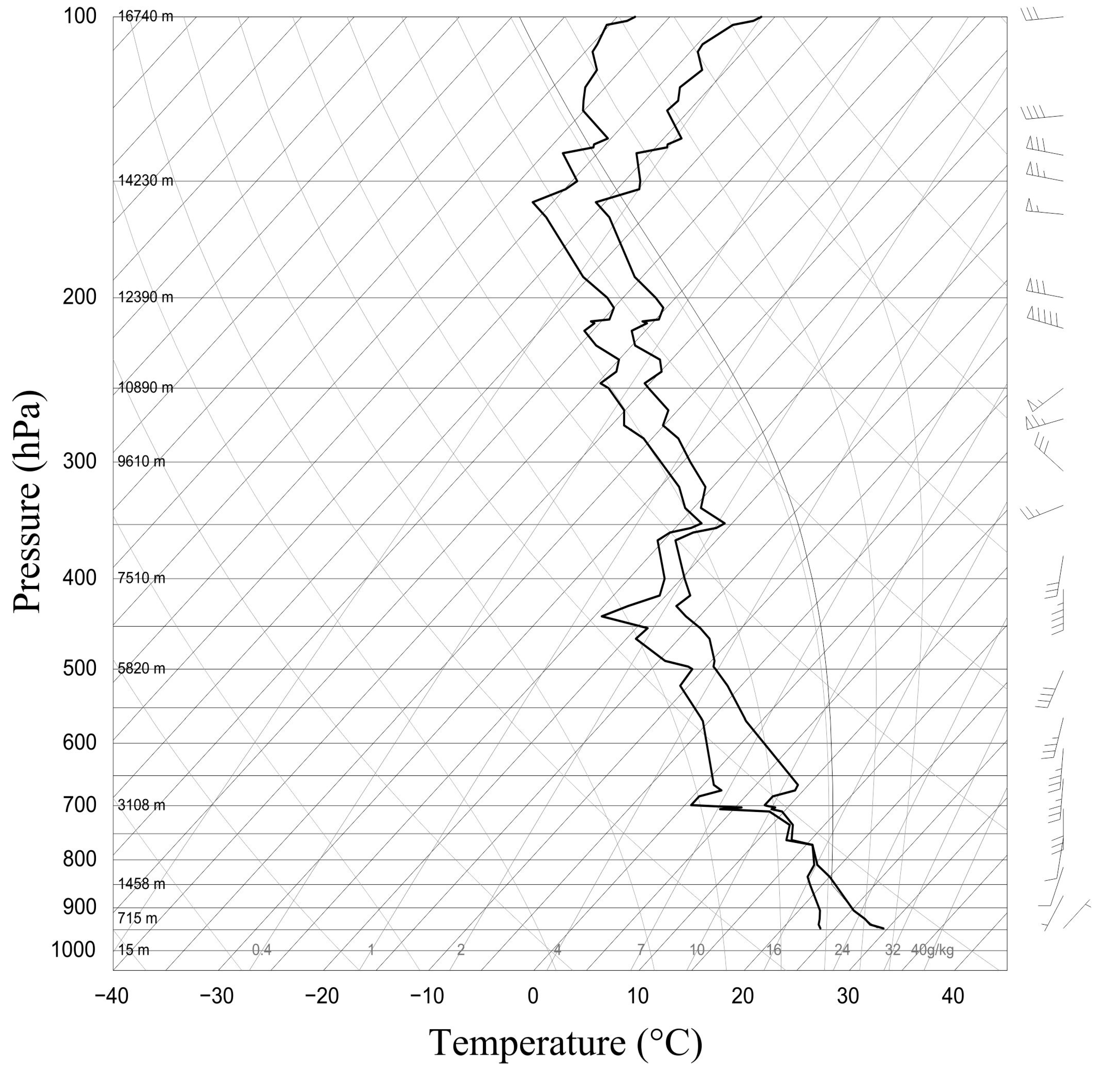
The initial, base state was horizontally homogeneous, time invariant and hydrostatically balanced, and it was initialized from a single sounding for Bismarck, North Dakota, USA, valid on 21 July 2014 at 21 h (Figure 1). The wind direction veered strongly (from NE to SSW direction) from the surface (0.5 km above mean sea level, AMSL) to 1.2 km AMSL. From 1.2 up to approximately 7.9 km AMSL the prevailing wind is characterized by S and SSW direction. Above this level, the prevailing wind blows between SW and NW direction. In the most part of the troposphere, the winds are very strong with the maximum wind intensity of 47 m s−1 located at approximately 11.9 km AMSL. A large amount of moisture is present until approximately 700 hPa (3.1 km AMSL). The maximum value of the water vapour mixing ratio is observed at the surface (19.82 g kg−1). The lifted condensation level (LCL) is located at approximately 1.28 km AMSL, where the air pressure is 867 hPa and temperature is approximately 21.5 °C. Thus, the LCL is situated at low level due to the high value of the water vapour mixing ratio. The value of convective available potential energy (CAPE) is very high (3401.7 J kg−1) and lifted index (LI) is quite low (−10.56 °C). For these reasons, this sounding is very favourable for development of severe hailstorms.

Figure 1.
Initial sounding of temperature (solid line) and dew-point (dashed line) plotted on skew T/log P diagram for Bismarck, North Dakota, USA, valid on 21 July 2014 at 21 h. Coordinate lines denote pressure (hPa) and temperature (°C). The height values and the wind barbs are shown on the right-hand side of the figure.
Convection was induced using an ellipsoidal warm bubble with a maximum temperature perturbation of 1.0 K in its centre. This bubble has a horizontal radius of 3000 m and a vertical radius of 800 m. The coordinates of the bubble centre are (x, y, z) = (52, 12, 1.3) km. Numerical experiments were performed over flat terrain (zflat = 0.5 km AMSL).
2.2. Model Microphysics
In the hailstorm model, numerical simulations are performed using two non-precipitating (cloud droplets and cloud ice crystals) and six precipitating hydrometeors (drizzle, raindrops, snow, graupel, frozen raindrops and hail). Three categories of liquid water (cloud droplets, drizzle and raindrops) use a unified Khrgian–Mazin size distribution [29] with corresponding lower and upper boundaries for these microphysics particles (see Table 1).

Table 1.
Minimum and maximum values for various categories of liquid drops.
The unified Khrgian–Mazin size distribution of the entire drop spectra (cloud droplets, drizzle and raindrops) is defined as
where A and B are parameters of the size distribution (1):
RM is the mean radius of the entire drop spectra:
where Q = qc + qd + qr is the total mixing ratio of the drops (cloud droplets, drizzle and raindrops); N = nc + nd + nr is the total concentration of the drops; qc (nc), qd (nd) and qr (nr) are the mixing ratios (number concentration) of the cloud water, drizzle and rain, respectively. Note parameters A and B are calculated from Q and RM in each time step. Q is calculated using prognostic variables qc, qd, qr. RM is obtained diagnostically from prognostic variables which include cloud droplet, drizzle and raindrop mixing ratios and corresponding number concentrations.
Further, A and B are used in production terms (e.g., Appendix A). Therefore, in the case of gravitional collection, A and B exist through the size distribution (1) in the rate of change of the mass PXY, and concentration level NPXY of particles Y due to their collisions with particles X:
where D represents the diameter of an individual particle, U(D) is its terminal velocity, EXY is the collection efficiency of particles Y for particles X, ρX is the density of a particle X, ρ is the air density and N(D) is size distribution of an individual particle. Minimum and maximum values for other hydrometeors are provided by Kovačević and Ćurić (2014) [28]. Cloud ice crystals are distributed in agreement with Hu and He (1988) [30]. Other hydrometeors are distributed in exponential form [31]. The terminal velocities for cloud droplets, raindrops, snow and graupel are given in agreement with Murakami (1990) [32]. The terminal velocity of drizzle category has the same form as for raindrops. The terminal velocity for cloud ice is obtained by Hu and He (1988) [30] and for frozen raindrops and hail by Wisner et al. (1972) [33]. A list of some constants and variables are provided in Appendix B. Other interactions between microphysical fields are described in more detail by Kovačević and Ćurić (2013, 2015) [7,27]. Figure 2 shows all microphysical processes and precipitation types in the model.
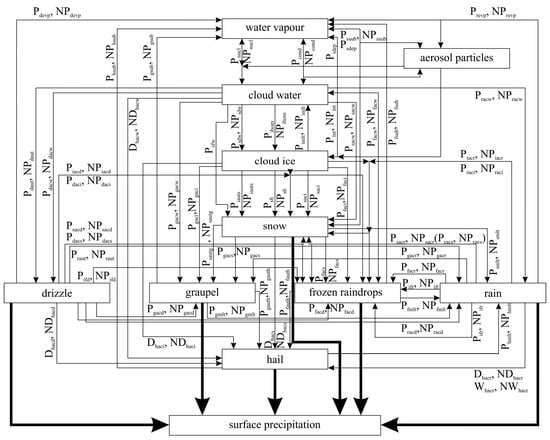
Figure 2.
Flow-chart showing all types of hydrometeors and the microphysical processes through which they originate and grow in the model we used in the experiment. PXY and NPXY depict the mass production rate and number concentration for corresponding microphysical process, respectively. Arrows show possible conversion directions. Bold arrows depict sedimentation of hydrometeors.
2.2.1. Cloud Droplet Activation
Cloud droplets are activated using a modified Twomey’s parameterization [34] by Cohard, et al. (1998) [35]. The concentration of cloud condensation nuclei (CCN) active on maximum supersaturation with respect to water (smax) is given as:
where C, k, β and µ are activation spectrum coefficients and 2F1(a, b, c; x) is the Gauss hypergeometric function [36]. The maximum supersaturation with respect to water smax is calculated iteratively as:
where w is vertical velocity of air, ρω is water density and B(x, y) is beta function. Some symbols (ψ1, ψ2, G) are described in more detail by Cohard et al. (1998) [35]. The number of newly formed cloud droplets per volume of air is equal to the difference of value obtained from the Equation (6) and a corresponding value from the previous time step [37] i.e.,
Cloud droplets will survive if they reach a critical diameter value Dcrit which is obtained from the Kohler curve equation (s − 1 = ak/r − bk/r3) i.e.,
where ak and bk are the coefficients for curvature and solute effect, respectively. Finally, if CCN are monodisperse distributed, the production rate for cloud water mixing ratio qc is:
In the model without drizzle particles, cloud droplets are transferred into rain category by autoconversion following Berry and Reinhardt (1974) [8].
2.2.2. Drizzle Representation
Drizzle particles are initiated due to the conversion of cloud droplets. Random mutual collision and coalescence of cloud droplets may result in the creation of larger droplets, which are recognized as drizzle in the model with drizzle category. The production rate for drizzle mixing ratio qd in one-parameter form is equal to autoconversion of cloud droplets to drizzle [38] (henceafter KK00) i.e.,
where rcm is mean radius (in microns) of cloud droplet population. If it is assumed that all newly initiated drizzle are of the same size, the production rate for drizzle number concentration will be
where ρ is air density and rd0 is radius of initiated drizzle. The scheme was originally developed for marine stratocumulus, but, due to the running model for convective clouds, we modified the scheme taking critical radius (rd0 = 100 µm) four times larger than that one in the original scheme KK00 (rd0 = 25 µm). This allows the presence of the larger average radius of cloud droplets. If the average cloud droplet is larger, the rate of production of drizzle (Pdaut) is higher, which should mean more cloud water turns into drizzle, and furthermore into rain. Considering the lifetime of a Cb cloud (approximately of 45 min to several hours) precipitation particles will be produced faster than in stratocumulus cloud (the lifetime of stratocumulus cloud is approximately from 6 to 12 h).
Once formed, drizzle continues to grow through the collision and coalescence with cloud droplets. The excess of drizzle amounts will be converted into raindrops by the autoconversion process. For this process we use a formulation similar to the Kessler (1969) [11] scheme for autoconversion of cloud to rain development:
but with modified values of autoconversion threshold, qd0, and proportionality constant α, and the production rate for rain number concentration in the following form:
Here, the Kessler modified scheme requires that drizzle mixing ratio reached a certain value before rain was produced. To get an autoconversion rate of typical order of magnitude in Cb clouds (10−4 kg kg−1 s−1) we choose qd0 of 2 × 10⁻⁴ kg kg−1 and α of 0.1 s−1, because drizzle content in the clouds is not as high as cloud water content. The threshold qd0 is arbitrarily defined by reducing its value toward the value which leads to rain production. Drizzle interactions with other hydrometeors (raindrops, cloud ice, snow, graupel, frozen raindrops and hail) lead to growing these hydrometeors and removing drizzle from cloud environment. These production rates are given in more detail in Appendix A.
3. Model Results and Discussion
3.1. Model Results
To examine the impact of drizzle on the microphysical and dynamic characteristics of hailstorm in this sensitivity study, we consider two special cases characterized by a different concentration of aerosols—clean and polluted air. Activation spectrum coefficients for nucleation of the liquid phase (referred to in Section 2) are summarized in Table 2 for clean and polluted cases (hereafter C and P, respectively).
Table 2.
Activation spectrum coefficients used for clean and polluted cases.
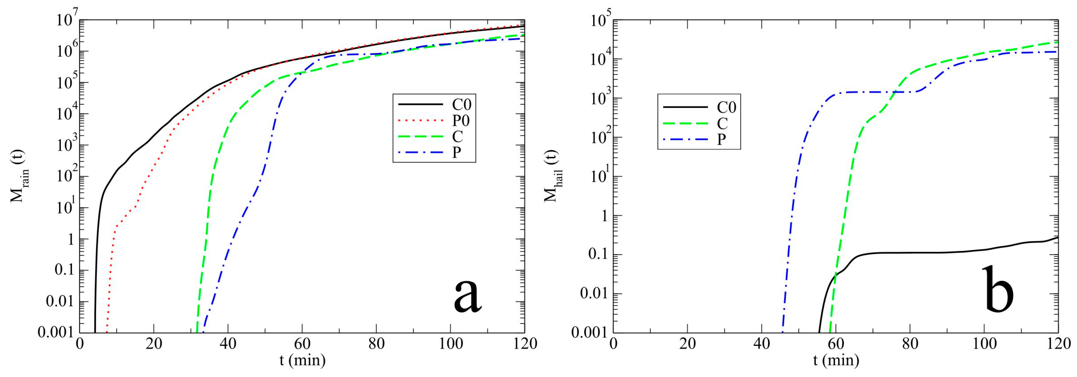
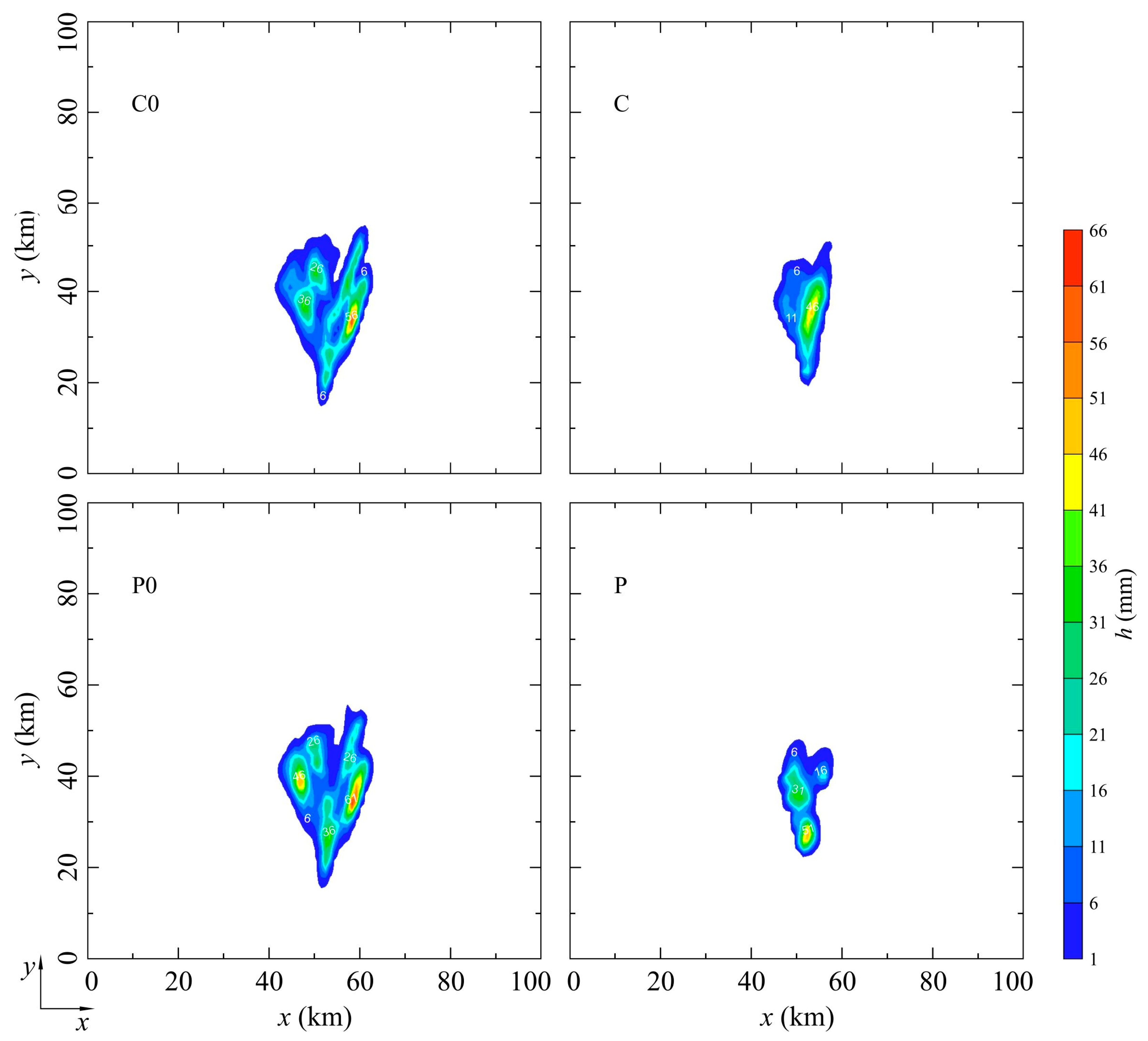
First, we consider the amount of precipitation on the ground. Figure 3 shows the amounts of total rain (Figure 3a) and hail (Figure 3b) at the surface as a function of time for clean (C, C0) and polluted cases (P0, P). In non-drizzle cases (the experiments C0 and P0), it can be seen that rain reaches the ground after a short time, from 4 to 8 min of the integration time. In simulations with drizzle, rain reached the ground after 30 min. The amounts of rain collected on the ground are lower in the case with drizzle particles. The presence of drizzle category in the model (the experiments C and P) produces significantly higher hail amounts in comparison with non-drizzle cases. It is notable from Figure 3b that the simulation with drizzle schemeinduces the appearance of hail on the ground for the experiment with polluted air andin the polluted case, occurrence of hail issomewhatearlier in time than that in clean case. A horizontal distribution of total surface precipitation after 120 min, for all simulations, is presented in Figure 4. For the experiments in drizzle mode, it can be noted that total accumulations are lower than in simulations without drizzle: the precipitating area is more narrow and is shifted slightly downwind.
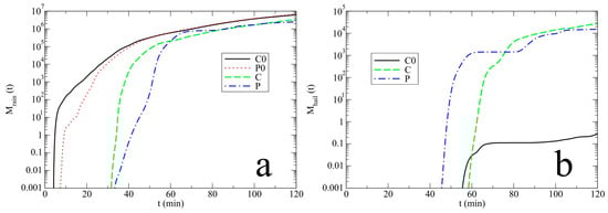
Figure 3.
The amounts (tonnes) of (a) surface rain and (b) hail as a function of time for experiments for clean air without drizzle (C0) and with drizzle (C) and polluted air without drizzle (P0) and with drizzle (P).
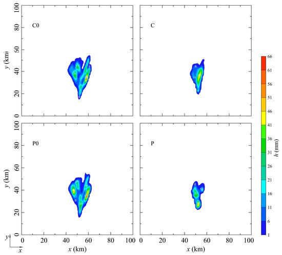
Figure 4.
Horizontal distribution of the total surface precipitation at t = 120 min for the non-drizzle and drizzle cases. Isohyets are drawn in intervals of 5 mm; the base isohyet is 1 mm. The amount of surface precipitation is depicted using a scale on the right-hand side of the figure.
3.2. Discussion
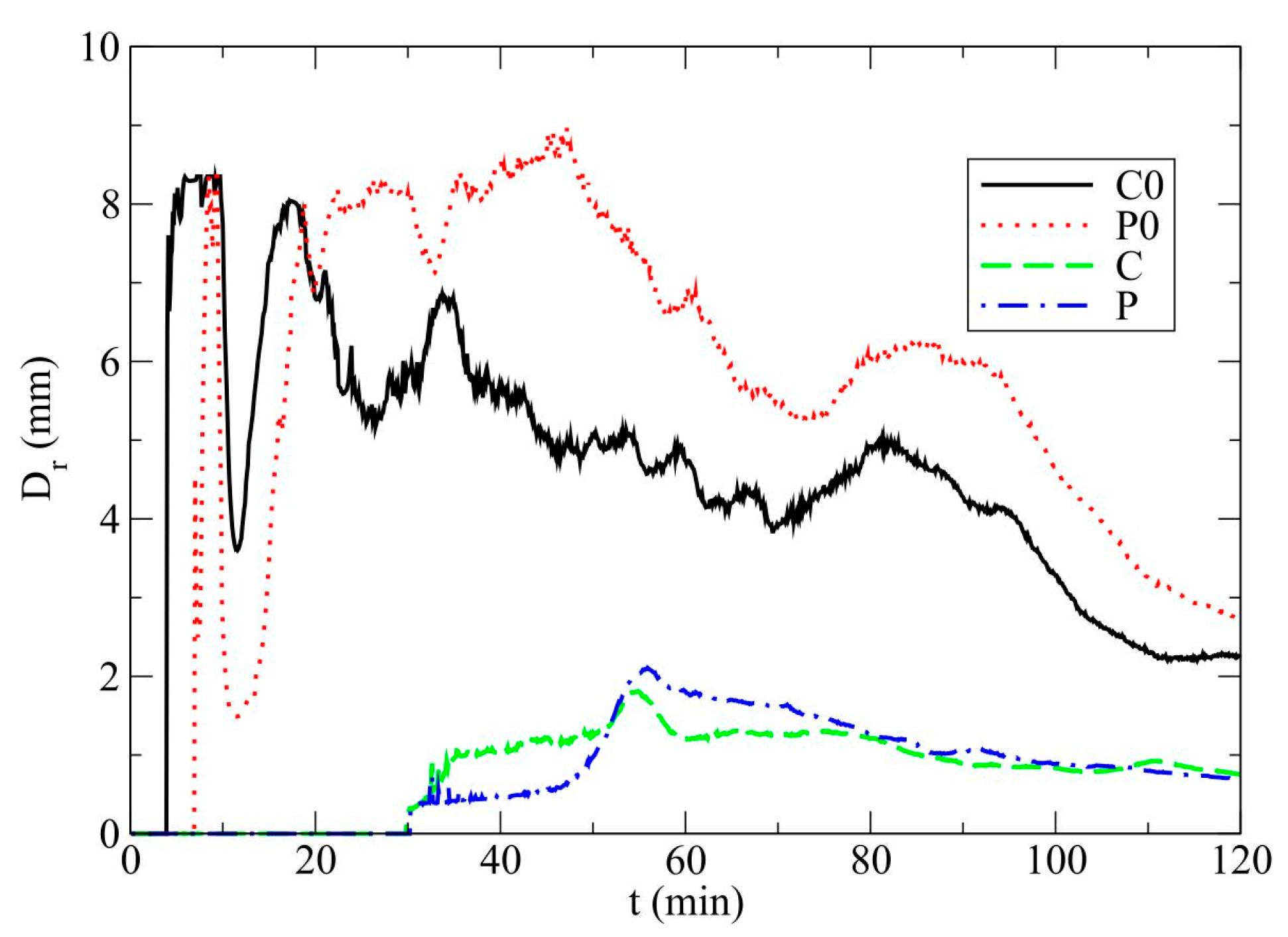
The addition of the drizzle category to the bulk microphysical scheme should produce a change in the raindrop size spectrum. Figure 5 shows the time evolution of the maximum values of the mean diameter (Dr in mm) of raindrops in the cases with (the experiments C and P) and without (the experiments C0 and P0) drizzle particles. It can be noted that the presence of drizzle category leads to decreasing of the size of raindrops. In drizzle cases, the sizes of the drops considered take values up to 2 mm in diameter most of the time, which is consistent with the typical size of raindrops. The alternate scheme generates raindrops greater than 4 mm in diameter for the most part of cloud life up to 96 and 105 min for the experiments C0 and P0, respectively. Raindrops take values up to about 8 mm in the maximum mean diameter (giant raindrops) and that is not consistent with common knowledge about the size of raindrops. Therefore, drizzle presence in the model leads to forming smaller raindrops.
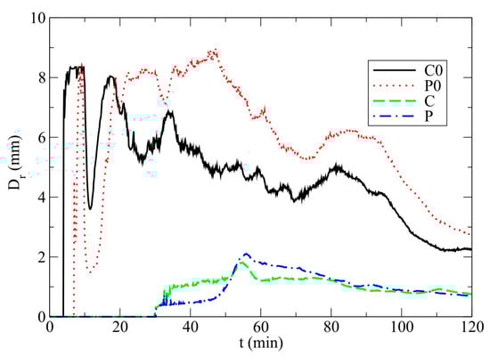
Figure 5.
The maximum values of the mean diameter of raindrop spectrum (mm) for clean air without drizzle (C0) and with drizzle (C) and polluted air without drizzle (P0) and with drizzle (P).
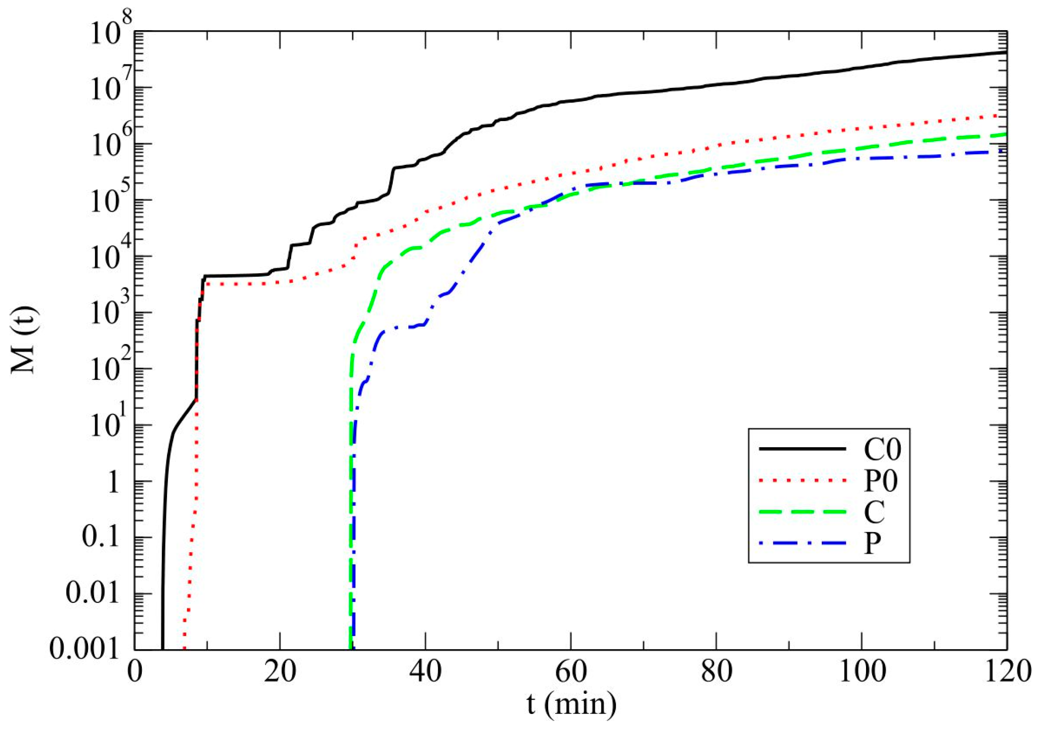
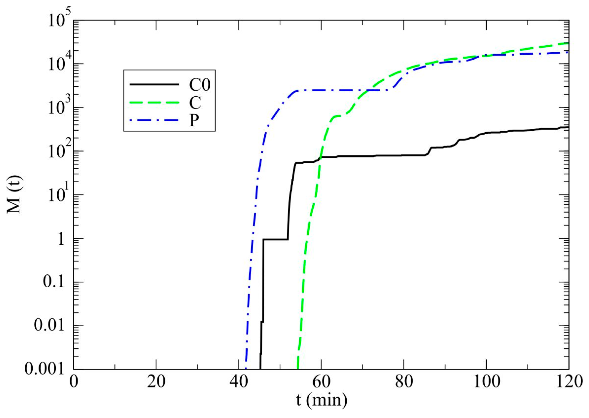
The mass contribution to rain (in tonnes) by the autoconversions of cloud droplets (non-drizzle cases) and drizzle (drizzle cases) as a function of time are depicted in Figure 6. Non-drizzle cases generate significantly more rain (especially in experiment C0) compared to drizzle counterparts indicating the importance of drizzle category in the model to the rain production. A population of drizzle similar in size (with similar terminal velocities) and with high number concentration reduces autoconversion to the raindrops in comparison with a significantly wider spectrum of cloud droplets in non-drizzle regime. Note, that in the absence of drizzle category rain occurs in the hailstorm very early, in fourth and seventh minute of initiation of convection, for C0 and P0, respectively. A time delay in raindrop formation in drizzle cases (of approximately 30 min) is caused by the phase development of liquid drops, which goes from cloud droplets through drizzle particles to the rain.
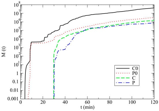
Figure 6.
As in Figure 5, but for the cumulative sum of the mass contribution, M (tonnes) to rain obtained by autoconversions of cloud droplets and of drizzle.
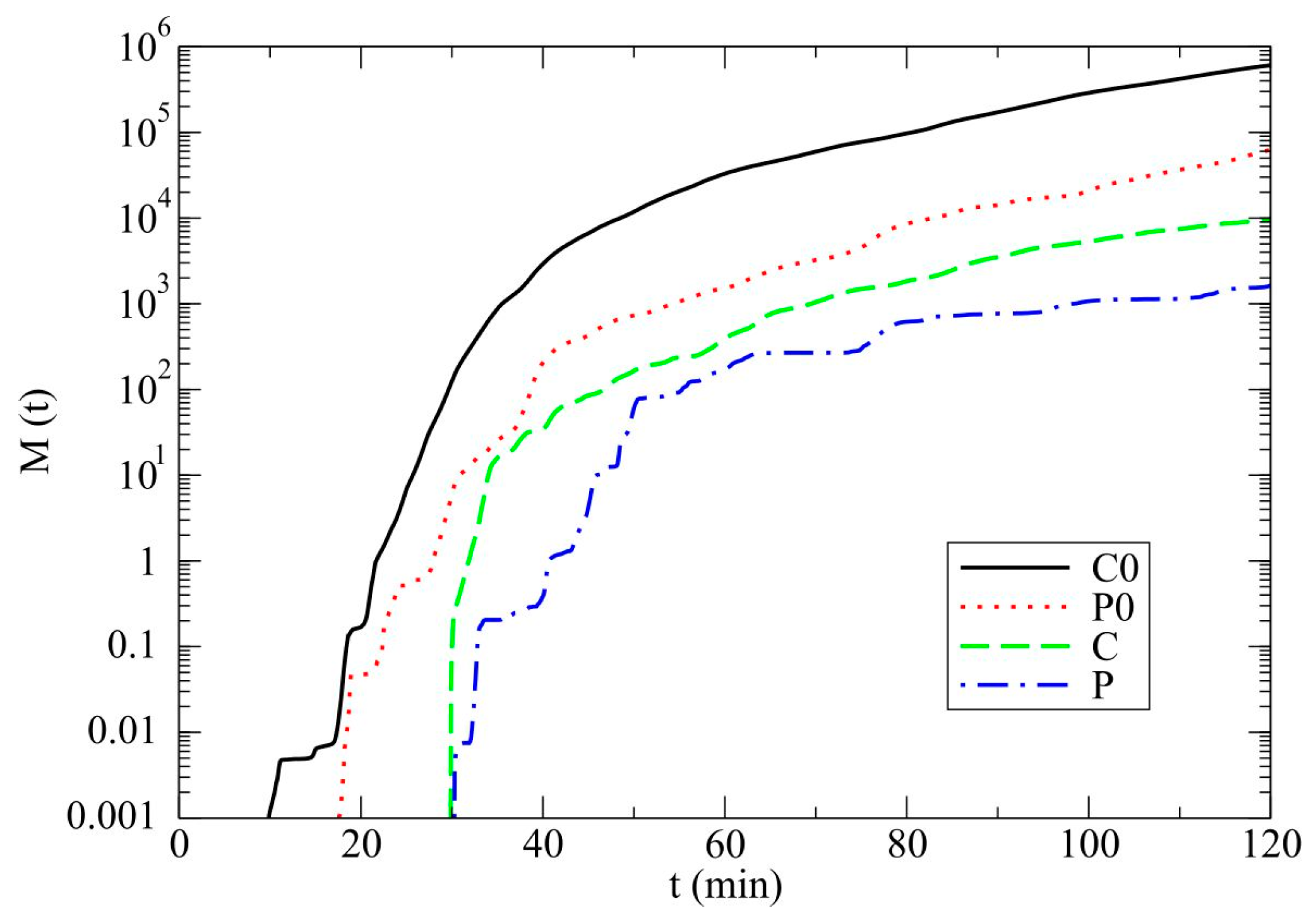
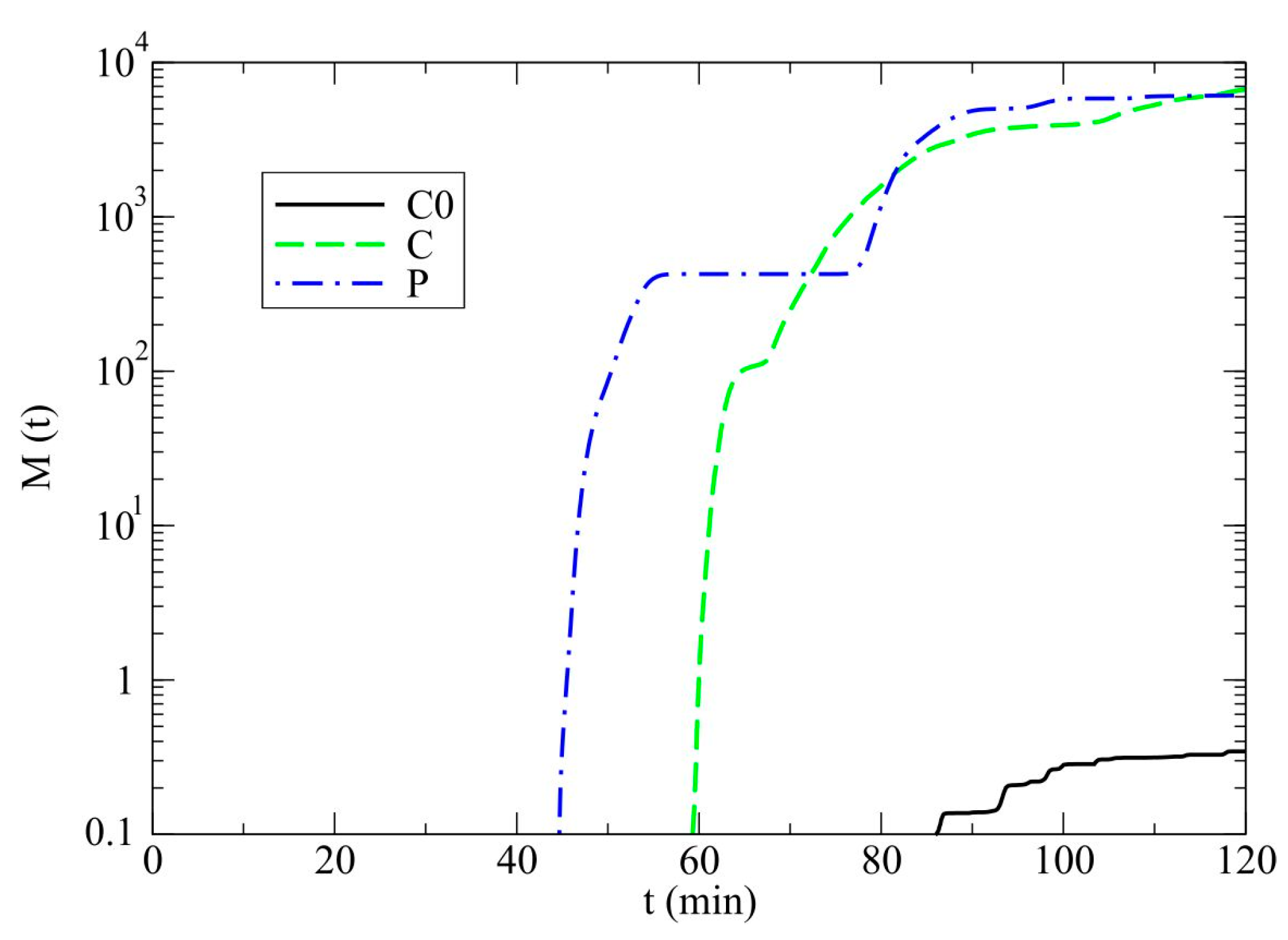
The mass contribution of the accretion of cloud droplets by raindrops as a function of time for all experiments is provided in Figure 7. In comparison with Figure 6, similar trends among non-drizzle and drizzle cases are obtained. Raindrops of smaller mean diameter (see Figure 5) are less efficient in collecting cloud droplets in comparison with much larger raindrops (with higher terminal velocities) which are generated by the non-drizzle regime. Therefore, a larger amount of cloud water remains present in the cloud volume in drizzle cases.
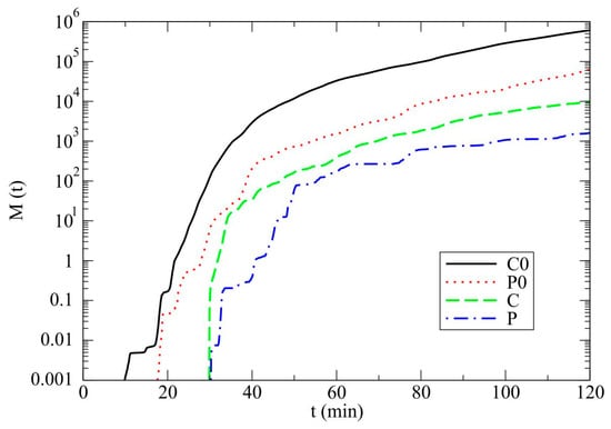
Figure 7.
As in Figure 5, but for the cumulative sum of the mass contribution, M (tonnes) to rain based on accretion of cloud droplets.
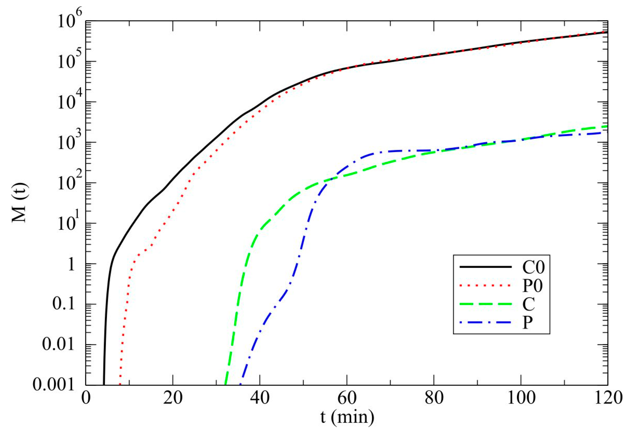
The mass contribution of evaporation of rain as a function of time, for all cases, is presented in Figure 8. In non-drizzle cases, an amount of evaporated rain is approximately three order magnitude greater than the corresponding amount in drizzle cases. This stronger sink leads to a smaller difference in surface precipitation amounts for all considered cases (Figure 3a).
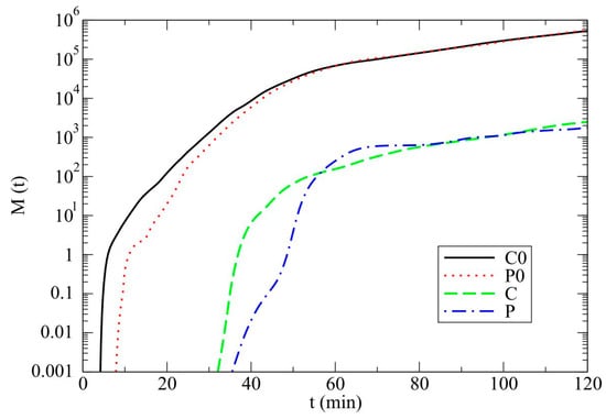
Figure 8.
As in Figure 5, but for the cumulative sum of rain evaporation (tonnes).
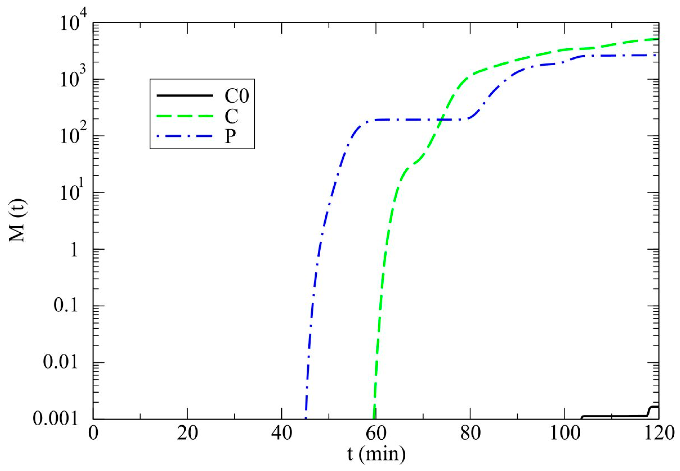
Figure 9 and Figure 10 show the initial production of the hail by the autoconversion of hailstone embryos (graupel and frozen raindrops) and the major production mechanism of hail growth—the accretion of cloud droplets onto hailstones, respectively. Figure 9 indicates that the drizzle category in the model contributes to hail production via autoconversions of graupel and frozen raindrops which does not exist in experiment P0.
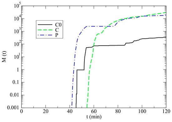
Figure 9.
As in Figure 5, but for the cumulative sum of the initial production of hail (tonnes) by autoconversion of hailstone embryos (graupel and frozen raindrops).
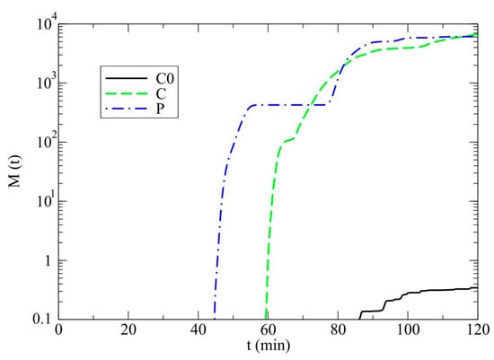
Figure 10.
As in Figure 5, but for the cumulative sum of the mass contribution, M (tonnes) to hail based on accretion of cloud droplets.
A scheme without drizzle does not favor production hailstone embryos in polluted conditions, which is in contradiction with the fact that there is a greater concentration of cloud droplets that should lead to stronger riming of ice particles and the formation of hail. Namely, the major production of hailstone embryos originates from their collections of cloud droplets. In a simulation of the hailstorm without a drizzle scheme, the lack of cloud water content due to rapid autoconversion of cloud droplets to rain (see Figure 6) will cause a decrease in growth of hailstone embryos. Similarly, an excess of cloud droplets will serve as a stronger source for growth of graupel and frozen raindrops via their accretion in drizzle cases. Consequently, the higher growth of these elements will lead to rapid autoconversion to hailstones. These conclusions can be applied to the growth process of hailstones via accretion of cloud droplets (Figure 10). Additionally, drizzle droplets will more strongly contribute to the growth of hail via their collisions and coalescences with hailstones in comparison with the corresponding collection of raindrops. Namely, in non-drizzle mode, raindrops have a greater mean diameter (see Figure 5) comparable to that typical for hail, which leads to similar terminal velocities, hence there should be a negligible accretion of rain by hail in these cases. Again, drizzle scheme supports the production of hail in both experiments, especially in cases related to the polluted air since hail is not produced in the experiment P0.
Figure 11 shows the melting amounts of hail, in tonnes, during the integration time, for all cases. It can be noted that the melting is stronger in the presence of drizzle category due to the hail formed in a higher amount in the experiment with than without drizzle. Thus, comparing all simulations, the final amounts of hail collected on the ground do not change a lot due to melting.
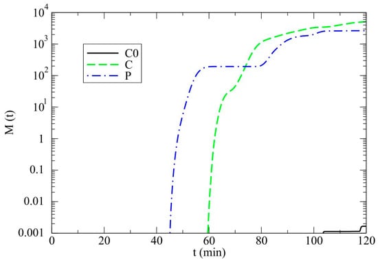
Figure 11.
As in Figure 5, but for the cumulative sum of hail melting (tonnes).
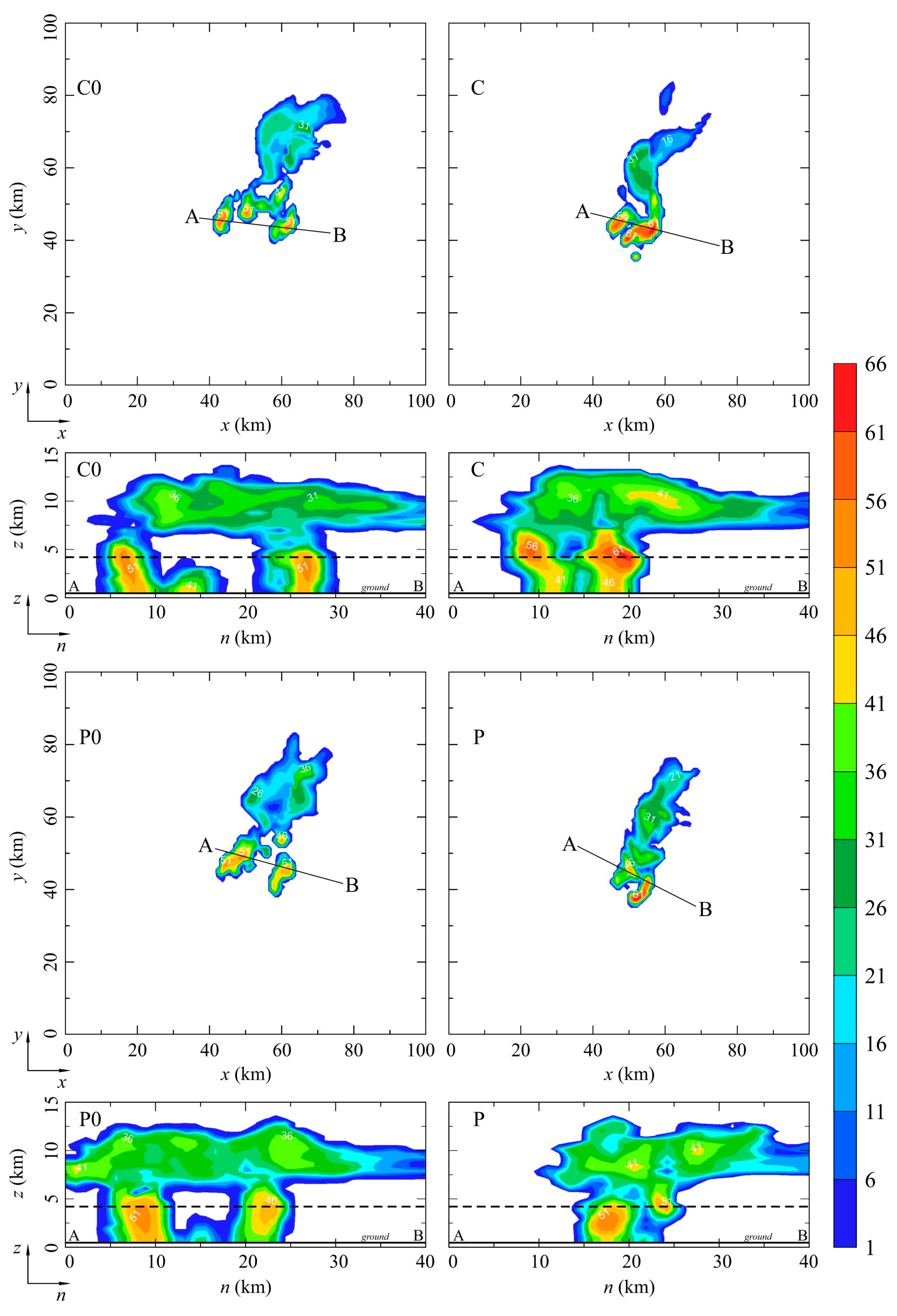
It could be useful to examine how the explicit presence of drizzle particles in the model affects the radar reflectivity factor–Z. In Figure 12, a horizontal (x-y) and vertical (n-z) cross-section of radar reflectivity factor at the end of the integration time for all experiments are presented.

Figure 12.
Radar reflectivity factor Z on horizontal and corresponding vertical cross-section at 120 min for the non-drizzle and drizzle cases. Horizontal distribution of Z is obtained for z = 4200 m. The corresponding vertical cross-section is obtained based on the line AB. Isolines are drawn in intervals of 5 dBZ; the base isoline is 1 dBZ. The Z-values are depicted using a scale on the right-hand side of the figure.
Line AB represents the horizontal axis, which indicates the position of the corresponding vertical cross-sections which are selected to be approximately perpendicular to mean direction of storm movement. For non-drizzle conditions, it can be seen that hailstorms are more widely spread and consist of several storm cells due to an earlier occurrence of storm splitting. In contrast, there are only two main storm cells in drizzle cases. Looking at the position of the main storm cells, it is of importance that the hailstorm moves slightly faster in simulations without drizzle than in the opposite case.
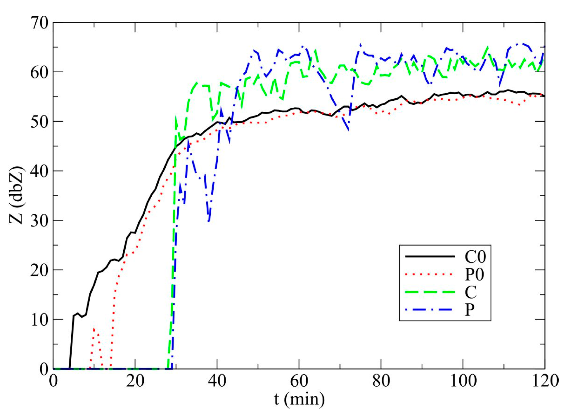
The value of radar reflectivity factor is generally higher in the model with included drizzle particles. It is more convincing in Figure 13, which represents the time evolution of the maximum value of radar reflectivity factor for all experiments. It can be noted that, after 30 min, the maximum value of Z is higher in the experiments with included drizzle particles. Typical values for Zmax range from 55 to 65 dBZ in drizzle cases as is usual for heavy rain and hail while Zmax in non-drizzle cases has lower values which implies absence of hail category. Radar reflectivity factor is proportional to the number of scattering elements and the sixth power of their diameters that means one drop of 3 mm in diameter has the same value of radar reflectivity factor as the population of 729 drops of 1 mm in diameter. Therefore, it is expected that the higher values of radar reflectivity factor characterize the non-drizzle conditions, which are favorable for generation of drops of larger mean sizes (see Figure 5).
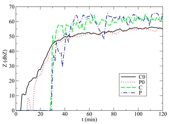
Figure 13.
As in Figure 5, but for the the maximum values of radar reflectivity factor Z (dBZ).
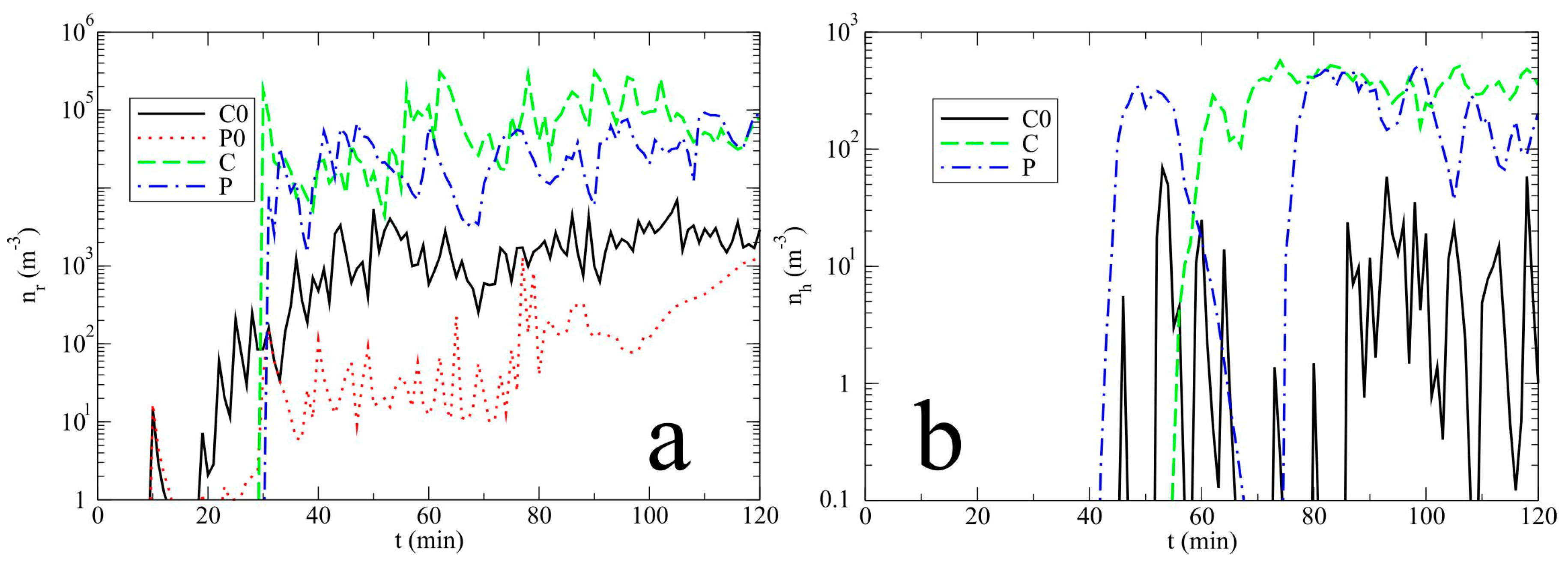
However, in the experiments with drizzle, significantly higher values of number concentration (approximately three orders of magnitude higher) of rain (Figure 14a) and hail (Figure 14b) lead to higher values of radar reflectivity factor compared to the experiments without drizzle. Thus, the impact of the number concentration on the Z-values overrides corresponding contribution of the size of scattered elements. Therefore, hailstorms with the explicit presence of drizzle are characterized by higher values of radar reflectivity factor. Further, the blue line (P) in Figure 13 shows two sudden decreases from 33–38 and 61–72 min. Namely, in these periods, raindrops are removed from the hailstorm to a greater extent (see Figure 14a). Typically, light rain occurs on the ground when the Z-value reaches 20 dBZ. However, in non-drizzle experiments, rain was observed on the ground (see Figure 3) despite the value of Z was lower than that one typical for onset of precipitation. Hence, the general conclusion should be that the radar reflectivity factor is not a good indicator of hailstorm characteristics in non-drizzle cases.
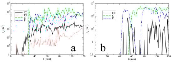
Figure 14.
As in Figure 3, but for the maximum number concentration (m−3) of (a) rain and (b) hail.
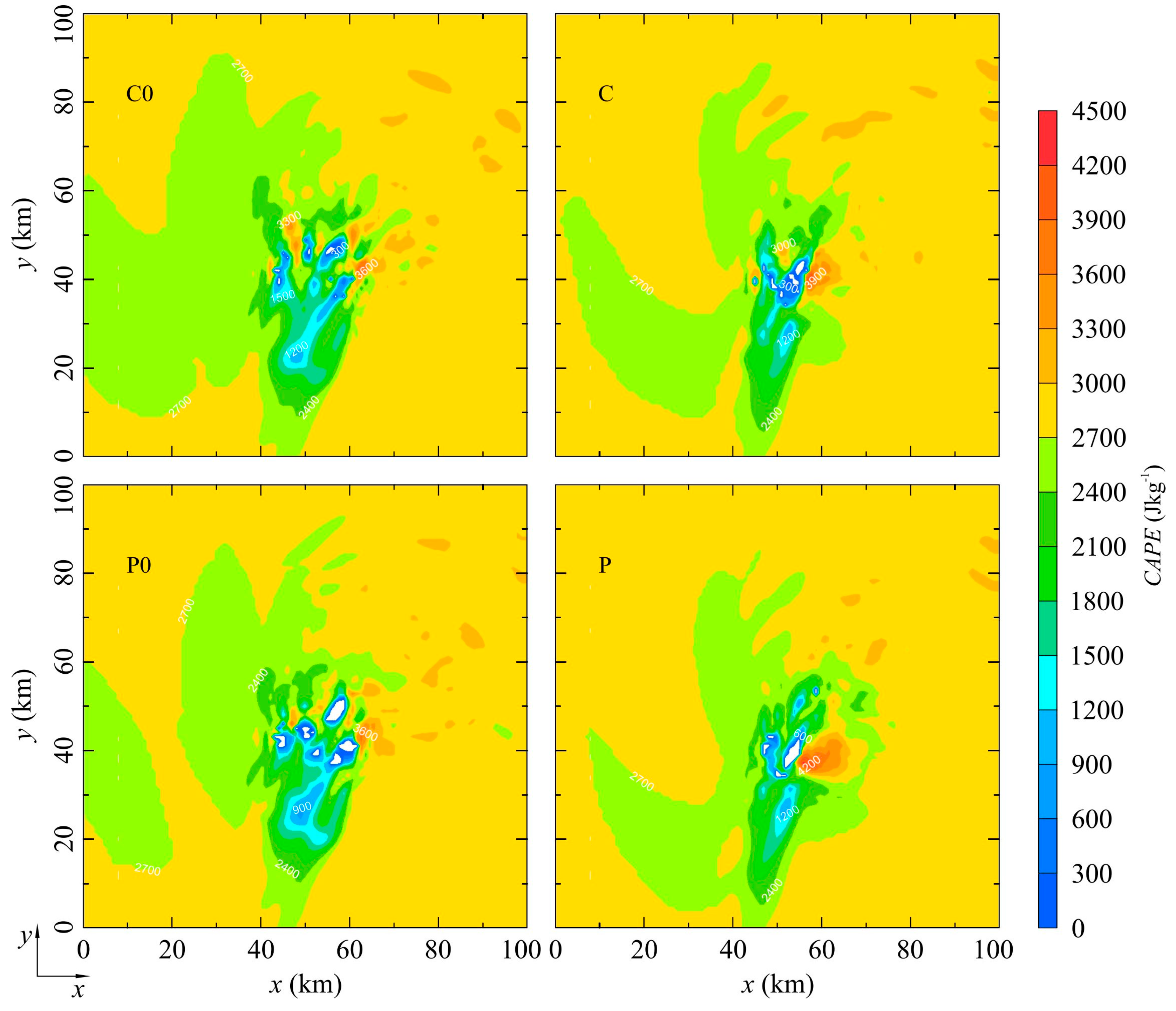
To describe the potential response of the atmosphere in the vertical direction to the changes caused by the hailstorm existence, we analysed the convective available potential energy (CAPE). Figure 15 shows the horizontal distribution of CAPE for all experiments. The value of CAPE at initial time was 3401.7 J kg−1. The non-shaded area refers to a zero value of CAPE. While the experiments with drizzle (C and P) are characterized by only one area of increased CAPE (CAPE > 3900 J kg−1), those without drizzle contribution (C0 and P0) show several corresponding areas which coincide with the regions of strong updrafts. At the same time, there are several widely spread areas with very low or equal to zero value of CAPE in non-drizzle cases. These areas could be associated with downdrafts induced by precipitation in a hailstorm. A higher quantity of accumulated rainfall over a larger area (see Figure 4) induces a wider area of downdrafts in these simulations. Additionally, significantly increased evaporation of rain in non-drizzle cases (see Figure 8) reduces the buoyancy of the air which further strengthens the downdrafts. In the experiments C and P, downdraft regions are narrower and less prominent. More numerous and similar in size drizzle particles contribute to damping of their autoconversion to rain. A slower autoconversion of drizzle to raindrops leads to lower values of precipitation amounts; hence, there are weaker and narrower regions with downdrafts.
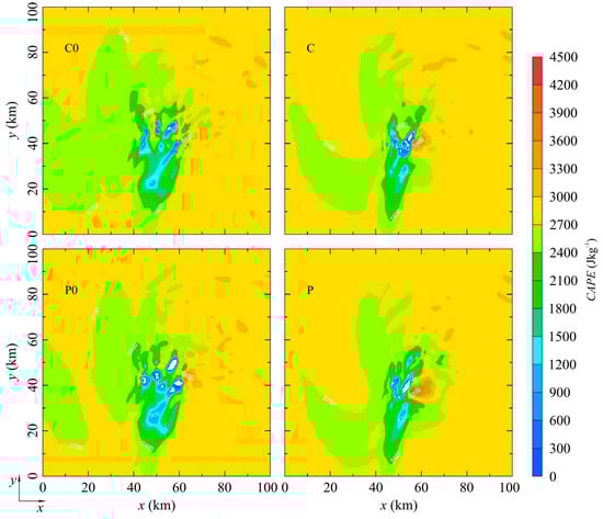
Figure 15.
Horizontal distribution of convective available potential energy (CAPE) at t = 120 min for the non-drizzle and drizzle cases. Isolines are drawn in intervals of 300 J kg−1; the base isoline is 0 J kg−1. The values of CAPE are depicted using a scale on the right-hand side of the figure. A non-shaded areas represent the value of 0 J kg−1.
4. Conclusions
In this preliminary study, we investigated the effects of the drizzle scheme on the surface precipitation and microphysical and dynamical characteristics of simulated hailstorm using the two-moment bulk microphysical scheme. Two specific cases (clean and polluted air) were discussed for conditions with and without drizzle scheme. As a separation between drizzle and cloud droplets and raindrops we used 0.2 and 0.5 mm, respectively. Drizzle drops are a subcategory of all liquid drops presented with the unified Khrgian-Mazin size distribution and expressed in terms of its mass and number concentrations.
Our main conclusions are as follows:
- The rain amounts on the ground are slightly lower in the absence of drizzle. In conditions with drizzle, a slower autoconversion of drizzle to rain and smaller accretion of cloud droplets by raindrops leads to weaker development of rain in a hailstorm and narrower rain bands at the surface.
- In simulations of a hailstorm in polluted cases that do not include the drizzle, there is no hail production.
- The mean diameters of raindrops are unrealistically large in non-drizzle cases in comparison with typical observed raindrops. In alternate cases, the values of the mean diameters of raindrops are consistent with common knowledge about size of raindrops.
- The drizzle case generates significantly more hail on the ground due to an excess of cloud droplets (due to slower accretion by rain) which may serve as a source for the hail growth via accretion of cloud droplets.
- Drizzle scheme causes a slightly greater value of radar reflectivity factor due to the fact that the impact of number concentration on the Z-values exceeds the corresponding impact of hydrometeor sizes in comparison with alternate cases. Noteworthy is the slightly faster movement of the hailstorm in simulations without drizzle category.
Analyzing the convective available potential energy, it can be concluded that downdrafts are significantly more developed and occupy wider areas in non-drizzle simulations of the hailstorm. The drizzle case generates weaker downdrafts due to a smaller autoconversion process of drizzle to rain and a less rain evaporation.
Acknowledgments
This research was supported by the Ministry of Education, Science and Technological Development of Serbia under Grant No. 176013.
Author Contributions
The sensitivity study has been performed in collaboration between all the authors. Nemanja Kovačević carried out sensitivity experiments, interpreted the model results and discussion and wrote the paper. Katarina Veljovic contributed to the interpretation of the model results and discussion and wrote the paper.
Conflicts of Interest
The authors declare no conflict of interest.
Appendix A
Accretion rates are determined by the integrand form of the stochastic collection equation using the “sweep-out” concept (following [31]). The production rate for mixing ratio PXY (kg kg−1 s−1) and number concentration NPXY (m−3 s−1) obtained from Equations (4) and (5) due to interactions of drizzle with other hydrometeors are given in Figure 2 and listed as follow:
- Collection of cloud water by drizzle is source for drizzle and sink for cloud water:where: F1 = 4, F2 = 4, F3 = 1.
- Collection of drizzle by rain is source for rain and sink for drizzle:where: E1 = 1, E2 = 2, E3 = 1.
- Collection of cloud ice by drizzle is source for frozen raindrops or for snow (if qi, qd < 10−4 kg kg−1) and sink for cloud ice and drizzle:
- Collection of drizzle by cloud ice is source for frozen raindrops or for snow (if qi, qd < 10−4 kg kg−1) and sink for cloud ice and drizzle:
- Collection of snow by drizzle is source for frozen raindrops or for snow (if qs, qd < 10−4 kg kg−1) and sink for snow and drizzle:
- Collection of drizzle by snow is source for frozen raindrops or for snow (if qs, qd < 10−4 kg kg−1) and sink for snow and drizzle:
- Collection of drizzle by graupel is source for graupel and sink for drizzle:
- Collection of drizzle by frozen raindrops is source for frozen raindrops and sink for drizzle:
- Collection of drizzle by hail is source for hail and sink for drizzle:
- Immersion freezing of drizzle is source for frozen raindrops and sink for drizzle:
- Drizzle evaporation is source for water vapour and sink for drizzle:
Appendix B
| Symbol | Description | Value | Units |
| λi | slope parameter for cloud ice | m−1 | |
| λs | slope parameter for snow | m−1 | |
| λg | slope parameter for graupel | m−1 | |
| λf | slope parameter for frozen raindrops | m−1 | |
| λh | slope parameter for hail | m−1 | |
| N0i | intercept parameter for cloud ice | m−5 | |
| N0s | intercept parameter for snow | m−4 | |
| N0g | intercept parameter for graupel | m−4 | |
| N0f | intercept parameter for frozen raindrops | m−4 | |
| N0h | intercept parameter for hail | m−4 | |
| ρ0 | standard air density | 1.225 | kg m−3 |
| ρs | density of snow | 102 | kg m−3 |
| ρh | density of hail | 917 | kg m−3 |
| a | constant for terminal velocity of rain | 842 | m0.2 s−1 |
| c | constant for terminal velocity of snow | 4.836 | m0.75 s−1 |
| e | constant for terminal velocity of cloud water | 3 × 10⁷ | m−1 s−1 |
| Avi | constant for terminal velocity of cloud ice | 3.249 | m2/3 s−1 |
| Avg | constant for terminal velocity of graupel | 124 | M0.36 s−1 |
| Ami | constant in formula for mass of cloud ice | 0.01 | kg m−2 |
| p0 | standard air pressure | 105 | N m−2 |
| p | air pressure | N m−2 | |
| T0 | freezing point of water | 273.16 | K |
| T | air temperature | K | |
| Symbol | Description | Value | Units |
| rd0 | radius of initiated drizzle particles | 100 | µm |
| Edw | collection efficiency of drizzle for cloud water | 1 | |
| Edr | collection efficiency of rain for drizzle | 1 | |
| Edi | collection efficiency of drizzle for cloud ice | 0.1 | |
| Eds | collection efficiency of drizzle for snow | 0.8 | |
| Egd | collection efficiency of graupel for drizzle | 0.8 | |
| Efd | collection efficiency of frozen raindrops for drizzle | 0.8 | |
| Ehd | collection efficiency of hail for drizzle | 0.8 | |
| A’ | constant in formula for immersion freezing | 0.66 | K−1 |
| B’ | constant in formula for immersion freezing | 100 | m−3 s−1 |
| g | gravity acceleration | 9.8 | m s−2 |
| CD | drag coefficient for hail | 0.6 | |
| Fk | (Lv/(RvT) − 1)Lvρw/(KaT) | m−2 s | |
| Fd | ρRvT/(eswDv) | m−2 s | |
| υ | kinematic viscosity of air | m2 s−1 | |
| Dv | diffusivity of water vapour in air | m2 s−1 | |
| Ka | thermal conductivity of air | W m−1 K−1 | |
| Lv | latent heat of evaporation | 2.5 × 10⁶ | J kg−1 |
| esw | pressure of saturated water vapour | N m−2 |
References
- Leroy, D.; Wobrock, W.; Flossmann, A.I. The role of boundary layer aerosol particles for the development of deep convective clouds: A high-resolution 3D model with detailed (bin) microphysics applies to CRYSTAL-FACE. Atmos. Res. 2009, 91, 62–78. [Google Scholar] [CrossRef]
- Khain, A.; Rosenfeld, D.; Pokrovsky, A.; Blahak, U.; Ryzhkov, A. The role of CCN in precipitation and hail in a mid-latitude storm as seen in simulations using a spectral (bin) microphysics model in a 2D dynamic frame. Atmos. Res. 2011, 99, 129–146. [Google Scholar] [CrossRef]
- Phillips, V.T.J.; Donner, L.J.; Garner, S.T. Nucleation processes in deep convection simulated by a cloud-resolving model with double-moment bulk microphysics. J. Atmos. Sci. 2007, 64, 738–761. [Google Scholar] [CrossRef]
- Milbrandt, J.A.; Morrison, H. Prediction of graupel density in a bulk microphysics scheme. J. Atmos. Sci. 2013, 70, 410–429. [Google Scholar] [CrossRef]
- Loftus, A.M.; Cotton, W.R.; Carrió, G.G. A triple-moment hail bulk microphysics scheme. Part I: Description and initial evaluation. Atmos. Res. 2014, 149, 35–57. [Google Scholar] [CrossRef]
- Ćurić, M.; Janc, D.; Vučković, V.; Kovačević, N. The impact of the choice of the entire drop size distribution function on Cumulonimbus characteristics. Meteorol. Z. 2009, 18, 207–222. [Google Scholar] [CrossRef]
- Kovačević, N.; Ćurić, M. Influence of drop size distribution function on simulated ground precipitation for different cloud droplet number concentrations. Atmos. Res. 2015, 158–159, 36–49. [Google Scholar] [CrossRef]
- Berry, E.X.; Reinhardt, R.L. An analysis of cloud drop growth by collection: Part II. Single initial distributions. J. Atmos. Sci. 1974, 31, 1825–1831. [Google Scholar] [CrossRef]
- Meyers, M.P.; Walko, R.L.; Harrington, J.Y.; Cotton, W.R. New RAMS cloud microphysics parameterization. Part II: The two-moment scheme. Atmos. Res. 1997, 45, 3–39. [Google Scholar] [CrossRef]
- Berry, E.X. Cloud droplet growth by collection. J. Atmos. Sci. 1967, 24, 688–701. [Google Scholar] [CrossRef]
- Kessler, E. On the distribution and continuity of water substance in atmospheric circulation. Meteorol. Monogr. 1969, 10, 88. [Google Scholar]
- Glickman, T.S. Glossary of Meteorology, 2nd ed.; American Meteorological Society: New York, NY, USA, 2000; p. 855. [Google Scholar]
- Wang, J.; Geerts, B. Identifying drizzle within marine stratus with W-band radar reflectivity. Atmos. Res. 2003, 69, 1–27. [Google Scholar] [CrossRef]
- Van Zanten, M.C.; Stevens, B.; Vali, G.; Lenschow, D.H. Observations of drizzle in nocturnal marine stratocumulus. J. Atmos. Sci. 2005, 62, 88–106. [Google Scholar] [CrossRef]
- Min, L.; Gong, W.; Liu, G.; Min, Q. Understanding the synoptic variability of stratocumulus cloud liquid water path over the Southeastern Pacific. Meteorol. Atmos. Phys. 2015, 127, 625–634. [Google Scholar] [CrossRef]
- Frisch, A.S.; Fairall, C.W.; Snider, J.B. Measurement of stratus cloud and drizzle parameters in ASTEX with a K-band Doppler radar and a microwave radiometer. J. Atmos. Sci. 1995, 52, 2788–2799. [Google Scholar] [CrossRef]
- Feingold, G.; Stevens, B.; Cotton, W.R.; Frisch, A.S. The relationship between drop in–cloud residence time and drizzle production in numerically simulated stratocumulus clouds. J. Atmos. Sci. 1996, 53, 1108–1122. [Google Scholar] [CrossRef]
- Gerber, H. Microphysics of marine stratocumulus clouds with two drizzle modes. J. Atmos. Sci. 1996, 53, 1649–1662. [Google Scholar] [CrossRef]
- Sears-Collins, A.L.; Schultz, D.M.; Johns, R.H. Spatial and temporal variability of nonfreezing drizzle in the United States and Canada. J. Clim. 2006, 19, 3629–3639. [Google Scholar] [CrossRef]
- Khain, A.; Pinsky, M.; Magaritz, I.; Krasnov, O.; Russchenberg, H.W.J. Combined observational and model investigations of the Z–LWC relationship in stratocumulus clouds. J. Appl. Meteorol. Clim. 2008, 47, 591–606. [Google Scholar] [CrossRef]
- Magaritz-Ronen, L.; Pinsky, M.; Khain, A. Drizzle formation in stratocumulus clouds: Effects of turbulent mixing. Atmos. Chem. Phys. 2016, 6, 1849–1862. [Google Scholar] [CrossRef]
- Hudson, J.G.; Yum, S.S. Maritime-Continental drizzle contrasts in small cumuli. J. Atmos. Sci. 2001, 58, 915–926. [Google Scholar] [CrossRef]
- Pujol, O.; Georgis, J.-F.; Sauvageot, H. Influence of drizzle on Z–M relationships in warm clouds. Atmos. Res. 2007, 86, 297–314. [Google Scholar] [CrossRef]
- Gerber, H.; Frick, G. Drizzle rates and large sea-salt nuclei in small cumulus. J. Geophys. Res. 2012, 117, D01205. [Google Scholar] [CrossRef]
- Gilmore, M.S.; Straka, J.M. The Berry and Reinhardt autoconversion parameterization: A digest. J. Appl. Meteorol. Clim. 2008, 47, 375–396. [Google Scholar] [CrossRef]
- Ćurić, M.; Janc, D.; Vučković, V. On the sensitivity of cloud microphysics under influence of cloud drop size distribution. Atmos. Res. 1998, 47–48, 1–14. [Google Scholar] [CrossRef]
- Kovačević, N.; Ćurić, M. The impact of the hailstone embryos on simulated surface precipitation. Atmos. Res. 2013, 132–133, 154–163. [Google Scholar] [CrossRef]
- Kovačević, N.; Ćurić, M. Sensitivity study of the influence of cloud droplet concentration on hail suppression effectiveness. Meteorol. Atmos. Phys. 2014, 123, 195–207. [Google Scholar] [CrossRef]
- Pruppacher, H.R.; Klett, J.D. Microphysics of Clouds and Precipitation, 2nd ed.; Kluwer: Dordrecht, The Netherlands, 1997; p. 954. [Google Scholar]
- Hu, Z.; He, G. Numerical simulation of microphysical processes in cumulonimbus—Part I: Microphysical model. Acta Meteorol. Sin. 1988, 2, 471–489. [Google Scholar]
- Lin, Y.-L.; Farley, R.D.; Orville, H.D. Bulk parameterization of the snow field in a cloud model. J. Appl. Meteor. 1983, 22, 1065–1092. [Google Scholar] [CrossRef]
- Murakami, M. Numerical modeling of dynamical and microphysical evolution of an isolated convective cloud—The 19 July 1981 CCOPE cloud. J. Meteorol. Soc. Jpn. 1990, 68, 107–127. [Google Scholar] [CrossRef]
- Wisner, C.; Orville, H.D.; Myers, C. A numerical model of a hail-bearing cloud. J. Atmos. Sci. 1972, 29, 1160–1181. [Google Scholar] [CrossRef]
- Twomey, S. The nuclei of natural cloud formation. Part II: The supersaturation in natural clouds and the variation of cloud droplet concentration. Geophys. Pure Appl. 1959, 43, 243–249. [Google Scholar] [CrossRef]
- Cohard, J.-M.; Pinty, J.-P.; Bedos, C. Extending Twomey’s analytical estimate of nucleated cloud droplet concentrations from CCN spectra. J. Atmos. Sci. 1998, 55, 3348–3357. [Google Scholar] [CrossRef]
- Gradshteyn, I.S.; Ryzhik, I.M. Table of Integrals, Series and Products, 7th ed.; Academic Press: New York, NY, USA, 2007; p. 1171. [Google Scholar]
- Cohard, J.-M.; Pinty, J.-P. A comprehensive two-moment warm microphysical bulk scheme. I: Description and tests. Q. J. R. Meteorol. Soc. 2000, 126, 1815–1842. [Google Scholar] [CrossRef]
- Khairoutdinov, M.; Kogan, Y. A new cloud physics parameterization in a large-eddy simulation model of marine stratocumulus. Mon. Weather Rev. 2000, 128, 229–243. [Google Scholar] [CrossRef]

© 2018 by the authors. Licensee MDPI, Basel, Switzerland. This article is an open access article distributed under the terms and conditions of the Creative Commons Attribution (CC BY) license (http://creativecommons.org/licenses/by/4.0/).