
Validation of ERA-Interim Precipitation Estimates over the Baltic Sea

Abstract
:1. Introduction
2. Data
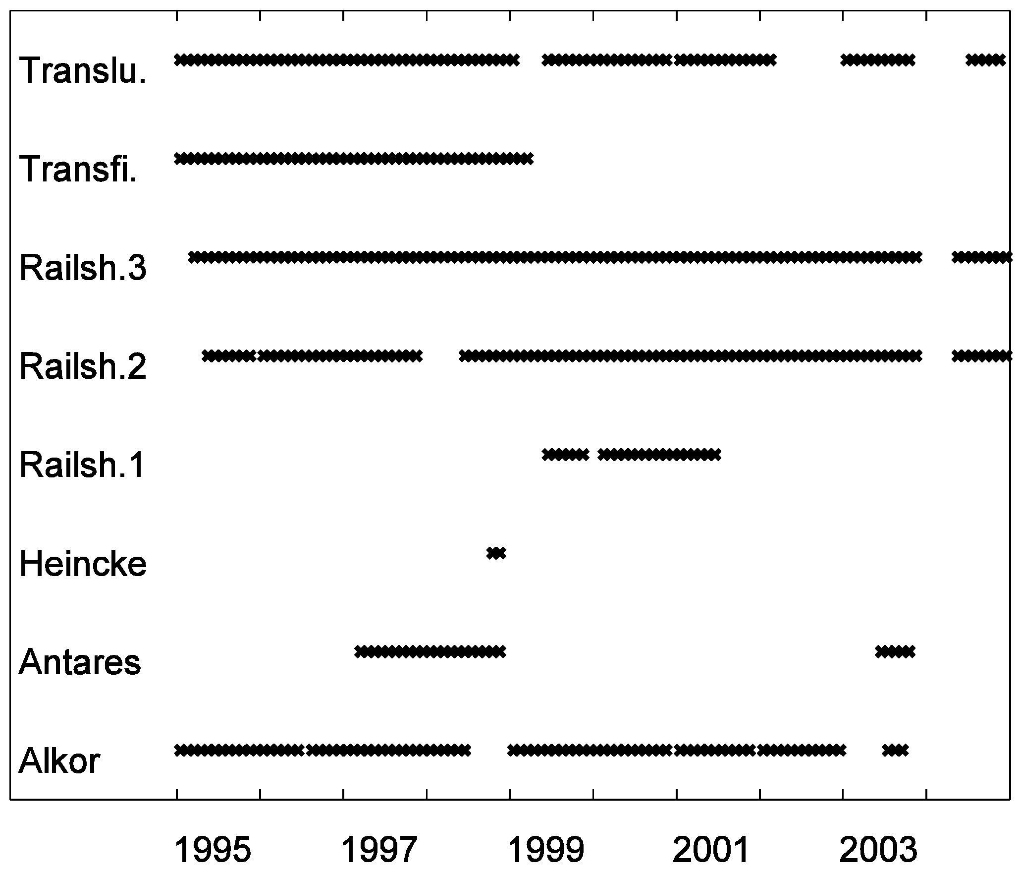
2.1. Ship Rain Gauge Measurements
2.2. ERA-Interim Reanalysis Precipitation Data
2.3. Supplementary Data ERA-Interim
2.4. Supplementary Marine Meteorological Data
2.5. Weather Radar Data
3. Method
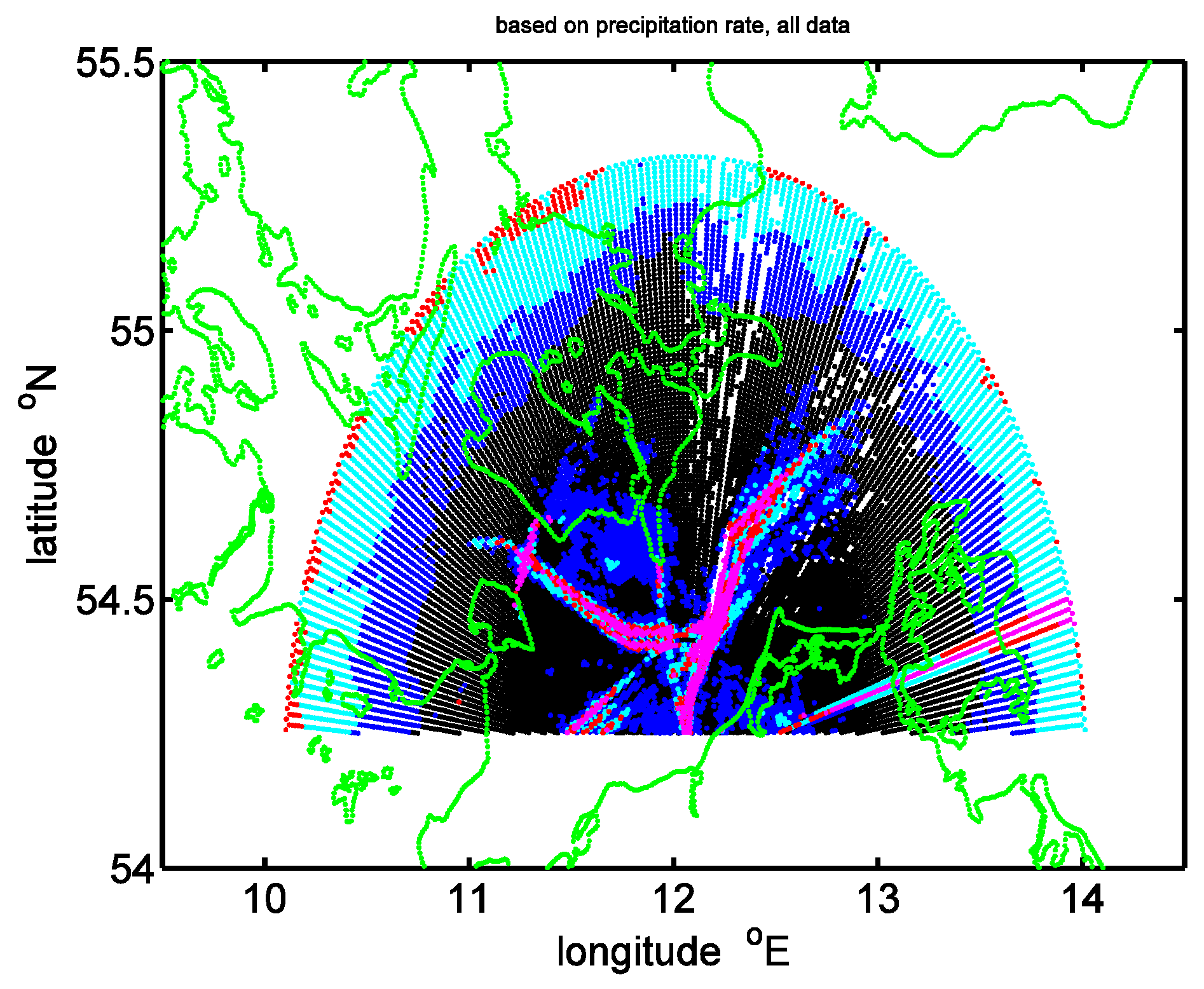
3.1. Collocation
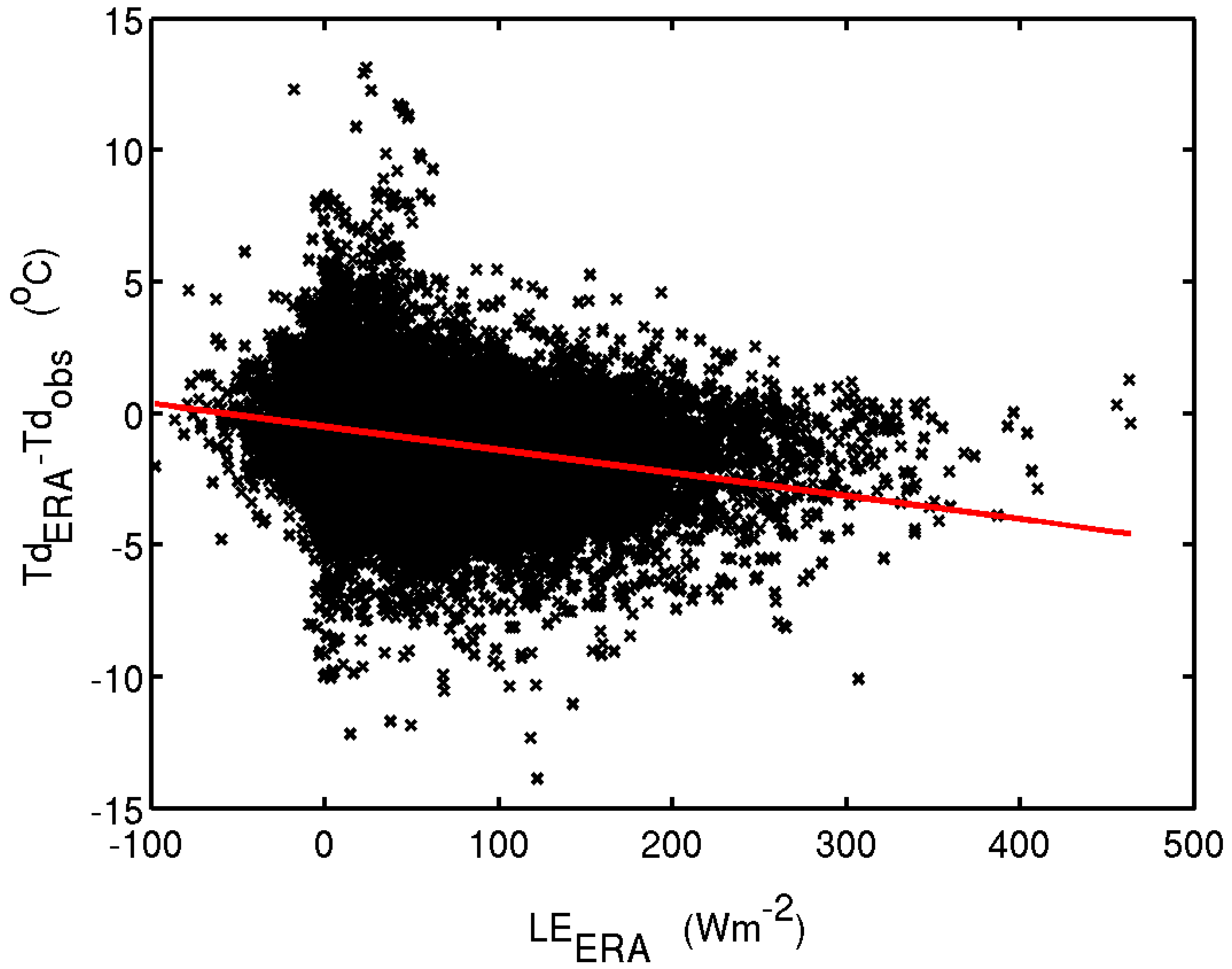
3.2. Stability and Latent Heat Fluxes
3.3. Simulations
3.4. Binary Statistics
4. Results
4.1. Binary Statistics
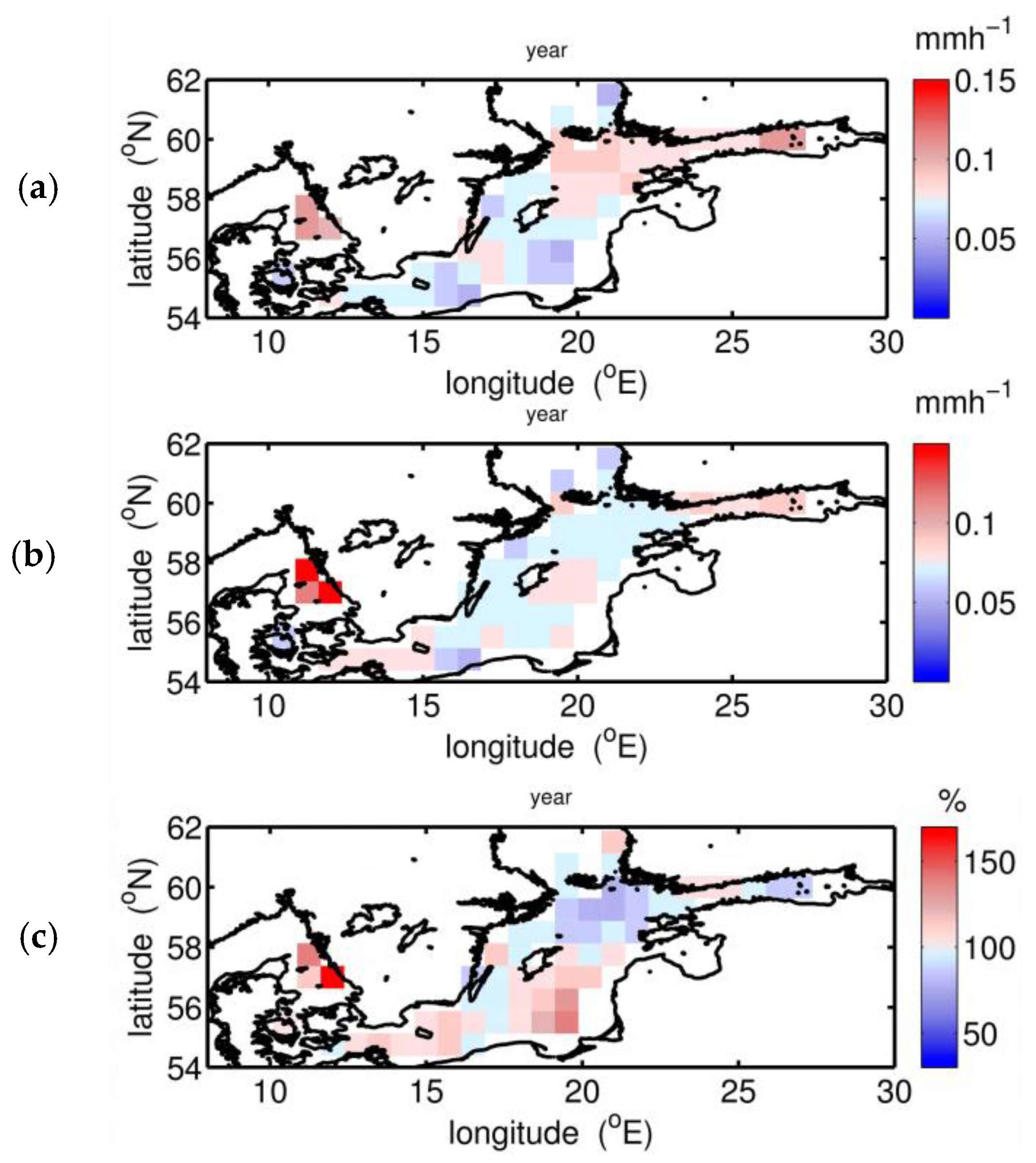
4.2. Annual Precipitation
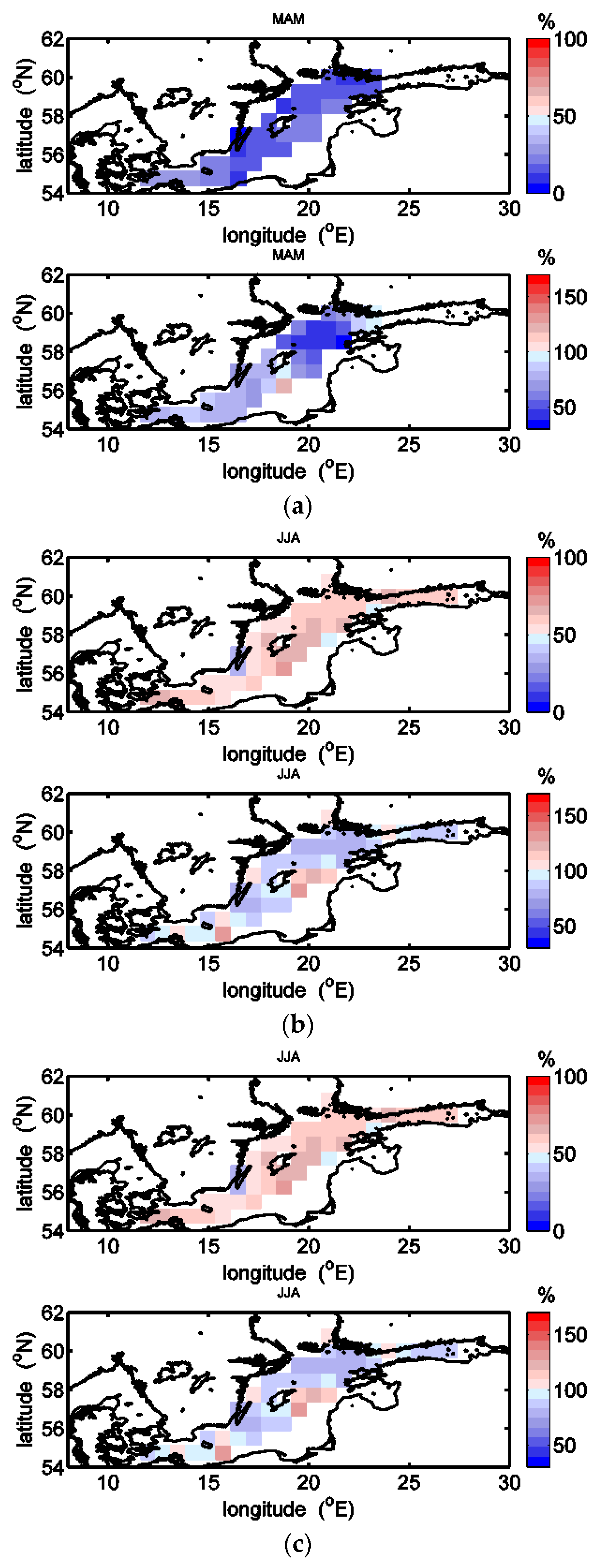
4.3. Seasonal Precipitation
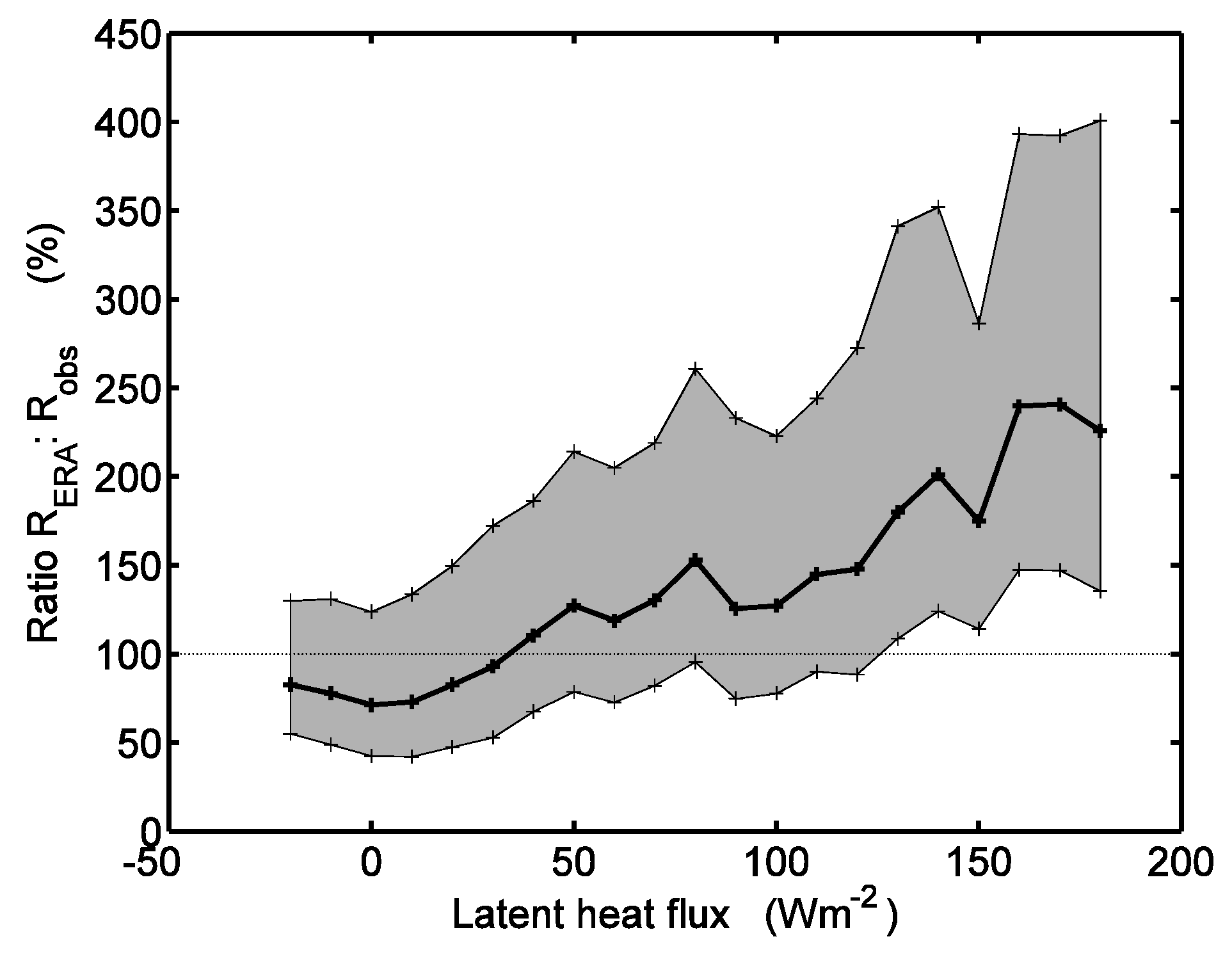
4.4. Influence of Stability on Precipitation
4.5. Fresh Water Budget P − E
5. Discussion
6. Conclusions
Acknowledgments
Conflicts of Interest
Abbreviations
| ECMWF | European Center of Medium Range Weather Forecast |
| BALTEX | The Baltic Sea Experiment |
| GPCP | Global Precipitation Climatology Project |
| HOAPS | Hamburg Ocean Atmosphere Parameters and Fluxes from Satellite Data |
| IMERG | Integrated Multi-satellitE Retrievals for Global precipitation measurement |
| GPS | Global Positioning System |
| IFS | Integrated Forecasting System |
| SWA | Seewetteramt Hamburg |
| DWD | German Weather Service |
| Z | Reflectivity |
| R | Rain rate |
| POD | Probability of detection |
| csi | Critical success index |
| p | Air pressure |
| T | Air temperature |
| Td | Dew point temperature |
| SST | Sea surface temperature |
| u | Wind speed |
| LE | Latent heat flux |
| P | Precipitation |
| E | Evaporation |
References
- Omstedt, A.; Elken, J.; Lehmann, A.; Leppäranta, M.; Meier, H.E.M.; Myrberg, K.; Rutgersson, A. Review progress in physical oceanography of the Baltic Sea during the 2003–2014 period. Prog. Oceanogr. 2014, 128, 139–171. [Google Scholar] [CrossRef]
- Smedman, A.-S.; Gryning, S.-E.; Bumke, K.; Högström, U.; Rutgersson, A.; Andersson, T.; Batchvarova, E. Precipitation and evaporation budgets over the Baltic Proper: Observations and modelling. J. Atmos. Ocean Sci. 2005, 10, 163–191. [Google Scholar] [CrossRef]
- Trenberth, K.E.; Fasullo, J.T.; Mackaro, J. Atmospheric moisture transports from ocean to land and global energy flows in reanalyses. J. Clim. 2011, 24, 4907–4924. [Google Scholar] [CrossRef]
- Dee, D.P.; Uppala, S.M.; Simmons, A.J.; Berrisford, P.; Poli, P.; Kobayashi, S.; Andrae, U.; Balmaseda, M.A.; Balsamo, G.; Bauer, P.; et al. The ERA-Interim reanalysis: Configuration and performance of the data assimilation system. Q. J. R. Meteorol. Soc. 2011, 137, 553–597. [Google Scholar] [CrossRef]
- Adler, R.F.; Huffman, G.J.; Chang, A.; Ferraro, R.; Xie, P.-P.; Janowiak, J.; Rudolf, B.; Schneider, U.; Curtis, S.; Bolvin, D.; et al. The version-2 global precipitation climatology project (GPCP) monthly precipitation analysis (1979–Present). J. Hydrometeorol. 2003, 4, 1147–1167. [Google Scholar] [CrossRef]
- Huffman, G.J.; Adler, R.F.; Arkin, P.; Chang, A.; Ferraro, R.; Gruber, A.; Janowiak, J.; McNab, A.; Rudolf, B.; Schneider, U. The global precipitation climatology project (GPCP) combined precipitation dataset. Bull. Am. Meteorol. Soc. 1997, 78, 5–20. [Google Scholar] [CrossRef]
- Andersson, A.; Fennig, K.; Klepp, C.; Bakan, S.; Graßl, H.; Schulz, J. The Hamburg Ocean atmosphere parameters and fluxes from satellite data—HOAPS-3. Earth Syst. Sci. Data 2010, 2, 215–234. [Google Scholar] [CrossRef]
- Andersson, A.; Klepp, C.; Fennig, K.; Bakan, S.; Graßl, H.; Schulz, J. Evaluation of HOAPS-3 ocean surface freshwater flux components. J. Appl. Meteorol. Climatol. 2011, 50, 379–398. [Google Scholar] [CrossRef]
- Huffman, G.J.; Bolvin, D.T.; Nelkin, E.J. Integrated Multi-satellitE Retrievals for GPM (IMERG) Technical Documentation. Available online: http://pmm.nasa.gov/sites/default/files/document_files/IMERG_doc.pdf (accessed on 26 April 2016).
- Rhein, M.; Rintoul, S.R.; Aoki, S.; Campos, E.; Chambers, D.; Feely, R.A.; Gulev, S.; Johnson, G.C.; Josey, S.A.; Kostianoy, A.; et al. Observations: Ocean. In Climate Change 2013: The Physical Science Basis; Stocker, T.F., Qin, D., Plattner, G.-K., Tignor, M., Allen, S.K., Boschung, J., Nauels, A., Xia, Y., Bex, V., Midgley, P.M., Eds.; Cambridge University Press: Cambridge, UK; New York, NY, USA, 2013; pp. 659–740. [Google Scholar]
- Belo-Pereira, M.; Dutra, E.; Viterbo, P. Evaluation of global precipitation data sets over the Iberian Peninsula. J. Geophys. Res. 2011, 116. [Google Scholar] [CrossRef]
- Thiemig, V.; Rojas, R.; Zambrano-Bigiarini, M.; Levizzani, V.; De Roo, A. Validation of satellite-based precipitation products over sparsely gauged African river basins. J. Hydrometeorol. 2012, 13, 1760–1783. [Google Scholar] [CrossRef]
- Wang, J.J.; Adler, R.F.; Huffman, G.J.; Bolvin, D.F. An updated TRMM composite climatology of tropical rainfall and its validation. J. Clim. 2014, 27, 273–284. [Google Scholar] [CrossRef]
- Hasse, L.; Großklaus, M.; Uhlig, K.; Timm, P. A ship rain gauge for use under high wind speeds. J. Atmos. Ocean. Technol. 1998, 15, 380–386. [Google Scholar] [CrossRef]
- Clemens, M. Machbarkeitsstudie zur Räumlichen Niederschlagsanalyse aus Schiffsmessungen Über der Ostsee. Ph.D. Thesis, Christian-Albrechts-Universität, Kiel, Germany, 2002. [Google Scholar]
- Clemens, M.; Bumke, K. Precipitation fields over the Baltic Sea derived from ship rain gauge on merchant ships. Boreal Environ. Res. 2002, 7, 425–436. [Google Scholar]
- Bumke, K.; König-Langlo, G.; Kinzel, J.; Schröder, M. HOAPS and ERA-Interim precipitation over sea: Validation against shipboard in situ measurements. Atmos. Meas. Tech. 2016, 9, 2409–2423. [Google Scholar] [CrossRef]
- Froidurot, S.; Zin, I.; Hingray, B.; Gautheron, A. Sensitivity of precipitation phase over the Swiss Alps to different meteorological variables. J. Hydrometeorol. 2014, 15, 685–696. [Google Scholar] [CrossRef]
- Kållberg, P. Forecast Drift in ERA-Interim ERA Report Series No 10. Available online: http://ecmwf.int/publications/ library/ecpublications/_pdf/era/era_report_series/RS_10.pdf (accessed on 11 April 2016).
- Berrisford, P.; Kållberg, P.; Kobayashi, S.; Dee, D.; Uppala, S.; Simmons, A.J.; Poli, P.; Sato, H. Atmospheric conservation properties in ERA-Interim. Q. J. R. Meteorol. Soc. 2011, 137, 1381–1399. [Google Scholar] [CrossRef]
- Over What Horizontal Area are Grid Point Data Values Valid? Available online: http://www.ecmwf.int/en/faq/over-what-horizontal-area-are-grid-point-data-values-valid (accessed on 6 April 2016).
- Sherwood, S.C.; Bony, S.; Dufresne, J.-L. Spread in model climate sensitivity traced to atmospheric convective mixing. Nature 2014, 505, 37–42. [Google Scholar] [CrossRef] [PubMed]
- Bumke, K.; Schlundt, M.; Kalisch, J.; Macke, A.; Kleta, H. Measured and parameterized energy fluxes for Atlantic transects of R/V Polarstern. J. Phys. Oceanogr. 2014, 44, 482–491. [Google Scholar] [CrossRef]
- Fairall, C.W.; Bradley, E.F.; Hare, J.E.; Grachev, A.A.; Edson, J.B. Bulk parameterization of air–sea fluxes: Updates and verification for the COARE algorithm. J. Clim. 2003, 16, 571–591. [Google Scholar] [CrossRef]
- Kent, E.C.; Woodruff, S.D.; Berry, D.I. Metadata from WMO publication No. 47 and an assessment of voluntary observing ship observation heights in ICOADS. J. Atmos. Ocean. Technol. 2007, 24, 214–234. [Google Scholar] [CrossRef]
- Rubel, F. Scale dependent statistical precipitation analysis. In Proceedings of the International Conference on Water Resources & Environment Research: Towards the 21st Century, Kyoto, Japan, 29–31 October 1996.
- Kinzel, J. Validation of HOAPS Latent Heat Fluxes against Parameterizations Applied to RV Polarstern Data for 1995–1997; Christian-Albrechts-Universität Kiel: Kiel, Germany, 2013. [Google Scholar]
- Obukhov, A.M. Turbulence in an atmosphere with a non-uniform temperature. Tr. Inst. Teor. Geofiz. Akad. Nauk. SSSR 1946, 1, 95–115. [Google Scholar] [CrossRef]
- Bartels, H.; Weigl, E.; Reich, T.; Lang, P.; Wagner, A.; Kohler, O.; Gerlach, N. in cooperation with the Meteo Solution GmbH RADOLAN, Routineverfahren zur Online-Aneichung der Radarniederschlagsdaten mit Hilfe von automatischen Bodenniederschlagsstationen (Ombrometer), DWD, Abteilung Hydrometeorologie, Zusammenfassender Abschlussbericht für die Projektlaufzeit von 1997 bis 2004. Available online: http://www.dwd.de/DE/leistungen/radolan/radolan_info/abschlussbericht_pdf.pdf;jsessionid=FC016CC6C87FB0CF48708E2EADBB847F.live11041?__blob=publicationFile&v=2 (accessed on 13 April 2016).
- Efron, B. Bootstrap Methods, another Look at the Jackknife. Ann. Stat. 1979, 7, 1–26. [Google Scholar] [CrossRef]
- WWRP/WGNE. Methods for Dichotomous Forecasts. Available online: www.cawcr.gov.au/projects/verification/#Methods_for_dichotomous_forecasts (accessed on 11 April 2016).
- Bechtholt, P. Atmospheric Moist Convection; ECMWF: Reading, UK, 2015.
- Hennemuth, B.; Rutgersson, A.; Bumke, K.; Clemens, M.; Omstedt, A.; Jacob, D.; Smedman, A.-S. Net precipitation over the Baltic Sea for one year using several methods. Tellus 2003, 55A, 352–367. [Google Scholar] [CrossRef]
- Holloway, C.E.; Petch, J.C.; Beare, R.J.; Bechtold, P.; Craig, G.C.; Derbyshire, S.H.; Donner, L.J.; Field, P.R.; Gray, S.L.; Marsham, J.H.; et al. Understanding and representing atmospheric convection across scales: Recommendations from the meeting held at Dartington Hall, Devon, UK, 28–30 January 2013. Atmos. Sci. Lett. 2014, 15, 348–353. [Google Scholar] [CrossRef]
- Lindau, R. Energy and water balance of the Baltic Sea derived from merchant ship observations. Boreal Environ. Res. 2002, 7, 417–424. [Google Scholar]
- Döscher, R.; Meier, H.E.M. Simulated sea surface temperature and heat fluxes in different climates of the Baltic Sea. AMBIO 2004, 33, 242–248. [Google Scholar] [CrossRef] [PubMed]
- Klepp, C. The Oceanic Shipboard Precipitation Measurement Network for Surface Validation—OceanRAIN. Atmos. Res. 2015, 163, 74–90. [Google Scholar] [CrossRef]


| ERA: No Rain | ERA: Rain | |
|---|---|---|
| ship: no rain measured | correct negatives 121,412 = 59.1% | false alarms 43,485 = 21.2% |
| ship: rain measured | misses 10,265 = 5.0% | hits 30,395 = 14.8% |
| Simulated Fields: No Rain | Simulated Fields: Rain | |
|---|---|---|
| simulated observations: no rain | correct negatives 27,321 = 83.6% | false alarms 3078 = 9.4% |
| simulated observations: rain | misses 549 = 1.7% | hits 1737 = 5.3% |
| ERA and Measurements | Simulated Data | |
|---|---|---|
| POD | 0.7475 | 0.7598 |
| csi | 0.3612 | 0.3238 |
| bias score | 1.8170 | 2.1063 |
| success ratio | 0.4114 | 0.3607 |
| accuracy | 0.7385 | 0.8890 |
| Parameter | Linear Regression | Mean Obs. | Mean ERA | Stand. Dev. | Corr. Coeff. |
|---|---|---|---|---|---|
| air pressure | pERA = 1.01·pObs − 10.04 hPa | 1013.5 hPa | 1013.4 hPa | 1.7 hPa | 0.98 |
| air temperature | TERA = 0.93∙TObs + 0.47 °C | 12.7 °C | 12.3 °C | 1.5 °C | 0.95 |
| dew point | TdERA = 0.98∙TdObs − 0.66 °C | 10.2 °C | 9.4 °C | 1.7 °C | 0.94 |
| SST | SSTERA = 0.96∙SSTObs + 0.17 °C | 12.8 °C | 12.4 °C | 1.5 °C | 0.96 |
| wind speed | uERA = 1.02∙uObs − 0.91 ms−1 | 5.6 ms−1 | 6.6 ms−1 | 2.7 ms−1 | 0.66 |
| latent heat flux | LEERA = 1.05∙LEObs + 3.62 Wm−2 | 39.4 Wm−2 | 45.0 Wm−2 | 36.0 Wm−2 | 0.75 |
| April/May | July/August | September/October | |
|---|---|---|---|
| P ERA-Interim | 36 mm·month−1 | 54 mm·month−1 | 62 mm·month−1 |
| P observation | 54 mm·month−1 | 57 mm·month−1 | 51 mm·month−1 |
| P - E ERA-Interim | 24 mm·month−1 | −2 mm·month−1 | −13 mm·month−1 |
| P - E observation | 44 mm·month−1 | 7 mm·month−1 | −16 mm·month−1 |
© 2016 by the author; licensee MDPI, Basel, Switzerland. This article is an open access article distributed under the terms and conditions of the Creative Commons Attribution (CC-BY) license (http://creativecommons.org/licenses/by/4.0/).
Share and Cite
Bumke, K. Validation of ERA-Interim Precipitation Estimates over the Baltic Sea. Atmosphere 2016, 7, 82. https://doi.org/10.3390/atmos7060082
Bumke K. Validation of ERA-Interim Precipitation Estimates over the Baltic Sea. Atmosphere. 2016; 7(6):82. https://doi.org/10.3390/atmos7060082
Chicago/Turabian StyleBumke, Karl. 2016. "Validation of ERA-Interim Precipitation Estimates over the Baltic Sea" Atmosphere 7, no. 6: 82. https://doi.org/10.3390/atmos7060082
APA StyleBumke, K. (2016). Validation of ERA-Interim Precipitation Estimates over the Baltic Sea. Atmosphere, 7(6), 82. https://doi.org/10.3390/atmos7060082