Bidimensional and Multidimensional Principal Component Analysis in Long Term Atmospheric Monitoring

Abstract

Atmospheric monitoring produces huge amounts of data. Univariate and bivariate statistics are widely used to investigate variations in the parameters. To summarize information graphs are usually used in the form of histograms or tendency profiles (e.g., variable concentration vs. time), as well as bidimensional plots where two-variable correlations are considered. However, when dealing with big data sets at least two problems arise: a great quantity of numbers (statistics) and graphs are produced, and only two-variable interactions are often considered. The aim of this article is to show how the use of multivariate statistics helps in handling atmospheric data sets. Multivariate modeling considers all the variables simultaneously and returns the main results as bidimensional graphs that are easy-to-read. Principal Component Analysis (PCA; the most known multivariate method) and multiway-PCA (Tucker3) are compared from methodological and interpretative points of view. The article demonstrates the ability to emphasize different information depending on the data handling performed. The results and benefits achieved using a more complex model that allows for the simultaneous consideration of the entire variability of the system are compared with the results provided by the simpler but better-known model. Atmospheric monitoring (SO₂, NO_x, NO₂, NO, and O₃) data from the Lake Como Area (Italy) since 1992 to 2007 were chosen for consideration for the case study.

1. Introduction

The effects of human activity on the atmosphere have been the subject of intensive studies in recent years as air pollution has been found to be connected closely to human health (see [1] and references therein). Moreover, at present time several international organizations are also devoted to deal with this important issue (World Health Organization WHO—www.who.int; US EPA Clean Air Act—www.epa.gov/clean-air-act-overview; EMEP/EEA air pollutant emission inventory guidebook—http://www.eea.europa.eu/themes/air/emep-eea-air-pollutant-emission-inventory-guidebook).

Atmospheric monitoring has led to a huge amount of data recorded all over the world through the years. Monitoring stations register hourly average data resulting in a huge amount of data when considering several months or years. Univariate and bivariate statistics are widely used to rationalize the information and frequently bidimensional graphs are employed to show them. The graphical approach allows for the explanation of simple to intricate patterns in an easy way, making the results available to scientists of different disciplines and also understandable to non-scientific individuals. Histograms (e.g., variable concentration vs. sampling site) and tendency profiles (e.g., variable concentration vs. time) are commonly used together with bidimensional plots in which two-variable correlations are taken into account. However, the univariate/bivariate statistical approach leads to at least two problems when dealing with big data sets. Firstly, to fully comprehend the system the large amount of numbers (statistics) and graphs that are produced have to be analyzed and compared. Secondly, only two-variable interactions are often considered, while a simultaneous investigation of all the variables is required to gain a complete description of the environment. Furthermore, the data handling and the interpretation of the results could be difficult using univariate/bivariate statistical tools due to the multivariate nature of the data in addition their large size.

The aim of this article is to propose a different way to add value to the data by bidimensional (two-way) and multidimensional (multiway) modeling techniques. These techniques allow all the sources of variation to be taken into account at once while also allowing hidden information in the data to be uncovered in a simple and swift way through the interpretation of only a few bidimensional plots.

In the literature the most employed technique is the Principal Component Analysis (PCA) [2,3,4,5,6,7], which allows for bidimensional data to be easily managed (e.g., different variables measured in several sampling sites or different variables measured over time for a particular sampling site (PCA could be classified as a two-way multivariate method)). However, when dealing with atmospheric monitoring (as in the majority of environmental monitoring contexts) chemico-physical parameters are usually monitored in different locations during a determined period, thus several variation sources could be identified. Sites × parameters × time (e.g., hours, days, years, etc.) could be arranged in at least a 3D array and even more dimensions could be investigated. Classical two-way calculation methods could be applied on the unfolded matrix with the following limitation: some variability sources will be confused (mixed) in one of the bidimensional data matrix dimensions.

Multiway methods gained a lot of attention in recent years in the environmental data analysis field (see [8,9,10,11,12] and references therein) as they represent a more appropriate choice when compared to bidimensional alternatives.

The case of study proposed here concerned an evaluation of the changes in the troposphere pollution in Lake Como Area (Northern Italy) through the investigation of some of its main pollutants. SO₂, NO_x, NO₂, NO (primary pollutants, directly emitted), and O₃ (secondary pollutant formed by a combination, or reaction, among primary pollutants) [13,14] were measured from the Regional Environmental Protection Agency (ARPA) by permanent troposphere analyzers over the period of 16 years. Thus, for this study, a huge data set was available.

In this work both two-way and multiway approaches were considered. A discussion about data transformation, preprocessing, and the theory of the multivariate methods considered is given in this article, as well as a discussion surrounding the results obtained by different data arrangements. Among the multidimensional methods (other multiway methods are described in ([15,16,17] and references therein)) the Tucker3 method (references follow) was chosen due to its fitting flexibility.

2. Experiments

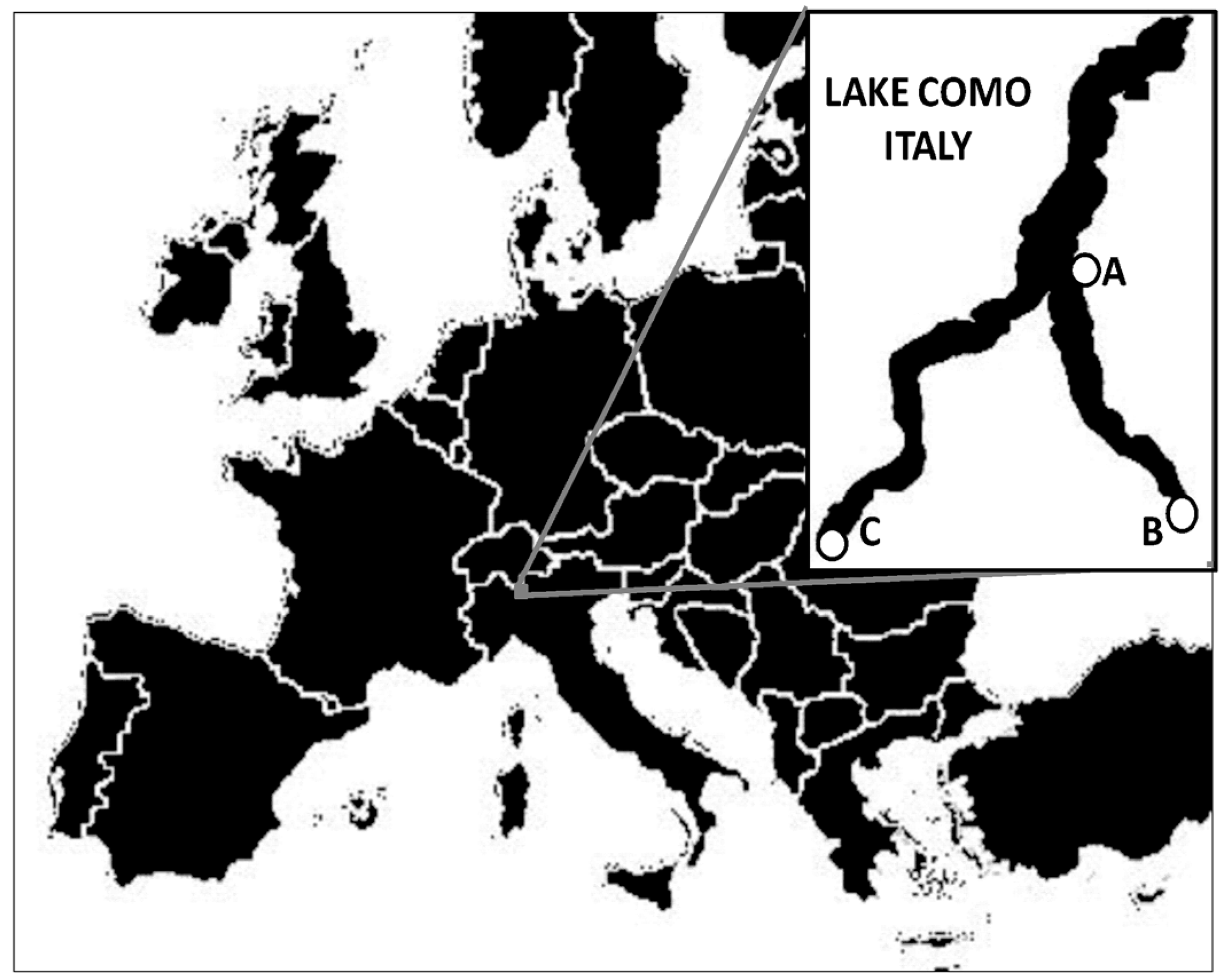
2.1. Case of Study

This study was focused on Lake Como Area (Lombardy, Northern Italy), which is an environmental and economic resource (especially for tourism) for the population living in North-West Lombardy: besides its importance as a drinking water reservoir the lake offers beautiful landscapes appreciated all over the world. This area is of relevant importance in the Italian environmental monitoring program.

Data considered in this study were obtained by troposphere analyzers which are permanently located in the cities of Como and Lecco, two high vehicular traffic sites, and Varenna, a small town situated in a rural area (Figure 1).

Specific locations of the troposphere analyzers follow: Como (labelled as C in the plot), longitude 9.06697886, latitude 45.81504217, 202 MSL; Lecco (labelled as B in the plot), longitude 9.39558125, latitude 45.85019631, 214 MSL; Varenna (labelled as A in the plot), loc. Perledo, longitude 9.28641942, latitude 46.01583272, 212 MSL.

The troposphere analyzer composition follows: pulsed fluorescence SO₂ analyzer (43C, Thermo Electron Corporation; LOD (limit of detection) 2.0 ppb-10 sec avg. time); UV analyzer (Teledyne API Model 400A; LOD < 0.6 ppb EPA definition) for O₃ measurements; chemiluminescence (Teledyne Instrument Model 200A; LOD 0.4 ppb) apparatus for NO_x, NO, and NO₂ measurements; Personal Computer for data elaboration and storage.

SO₂, NO_x, NO₂, NO, and O₃ concentration values (average per hour—stored only if the measurement in continuum was provided for at least 75% of the period of one hour, if not the machine stored an arbitrary code to identify a missing datum) were available from 1 January 1992 to 31 December 2007.

2.2. Theory

2.2.1. Raw Data: Transformation and Preprocessing

Bilinear models (e.g., PCA) assume linear data: the presence of skewed variables in the dataset has to be checked and eventually corrected. Data transformation returns variable distributions suitable for a powerful analysis [18]. Instead, data preprocessing allows an easier extraction of the meaningful information by reducing effects such as, for example, measurements in different units and variables with different variance values (e.g., magnitude order).

• Average
  The models were built on averaged data, according to the information to be emphasized, as described in following sections. Average values were calculated only if 75% of the data were available (following the criteria used from the troposphere analyzer), any datum that did not meet this criteria was coded as missing value.
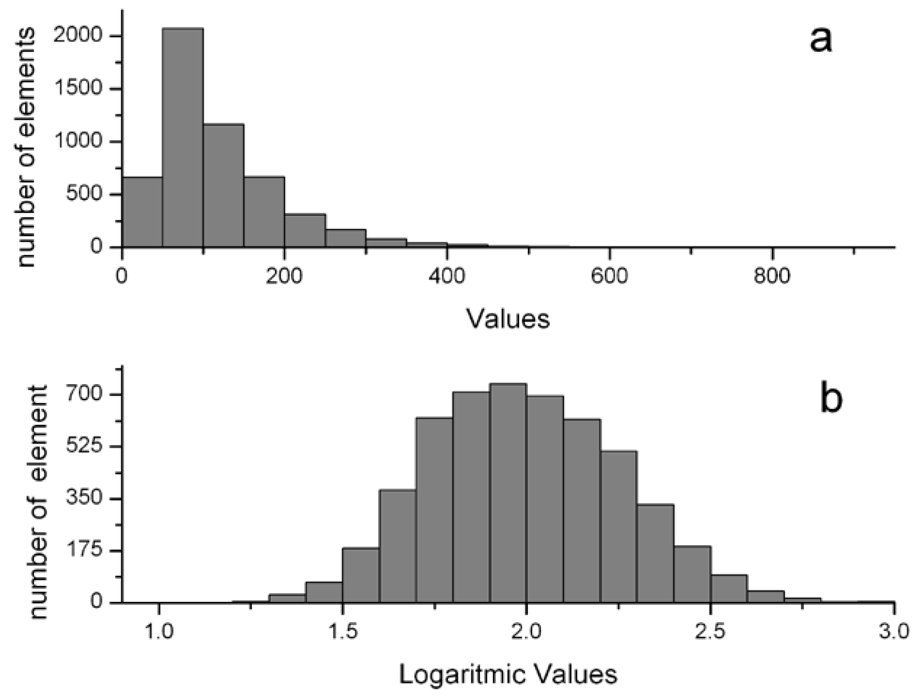
• Logarithmic transformation
  Variables box plots and histogram plots were analyzed to check non-linearities. An example of a highly asymmetrical variable is shown in Figure 2a. In such cases, a data logarithmic transformation, or a square root in the case of slight asymmetry, was applied to make the distribution more symmetrical. Figure 2b shows the same variable distribution after a logarithmic transformation.
• Autoscaling
  This preprocessing technique is required when variables expressed in different units and/or showing different variation ranges have to be compared. It gives all variables the same chance to influence the estimation of the components. Autoscaling results from performing the mean centering and the standardization transformations:

  $$x_{ij}^{autoscale}=\frac{x_{ij}^{original}-\overline{x_j}}{s_j}$$
• J-scaling
  J-scaling is the autoscaling in the variable (columns) direction in multi-way modeling [8,19]: the objects with all the other information are arranged in the rows. This pretreatment removes the differences between the variables arising from different ranges and magnitudes giving all of the variables the same chance to contribute to the model. This method retains the differences between the objects.

2.2.2. Bidimensional Modeling: Principal Component Analysis

The aim of the Principal Component Analysis (PCA) [20,21] is the extraction and synthesis of the relevant information from the data by transforming the original variables into new variables called Principal Components (PCs). They are linear combinations of the original variables; as they are orthogonal, each of them carries independent information. A value of explained variance is associated to each of the principal components. This value is complementary, quantifiable and in decreasing order: the first component explains the greater percentage of variance, the second one explains it at a lower degree, the third one to a still lower value, and so on, until the last members only contribute to the model noise. PCA calculation produces diagrams called score and loading plots. In the score plot groups of objects, trends, and outliers can be visualized; the Loading Plot shows the correlation between the variables. Variables with a high absolute value on a certain PC have a larger contribution to the construction of the given PC.

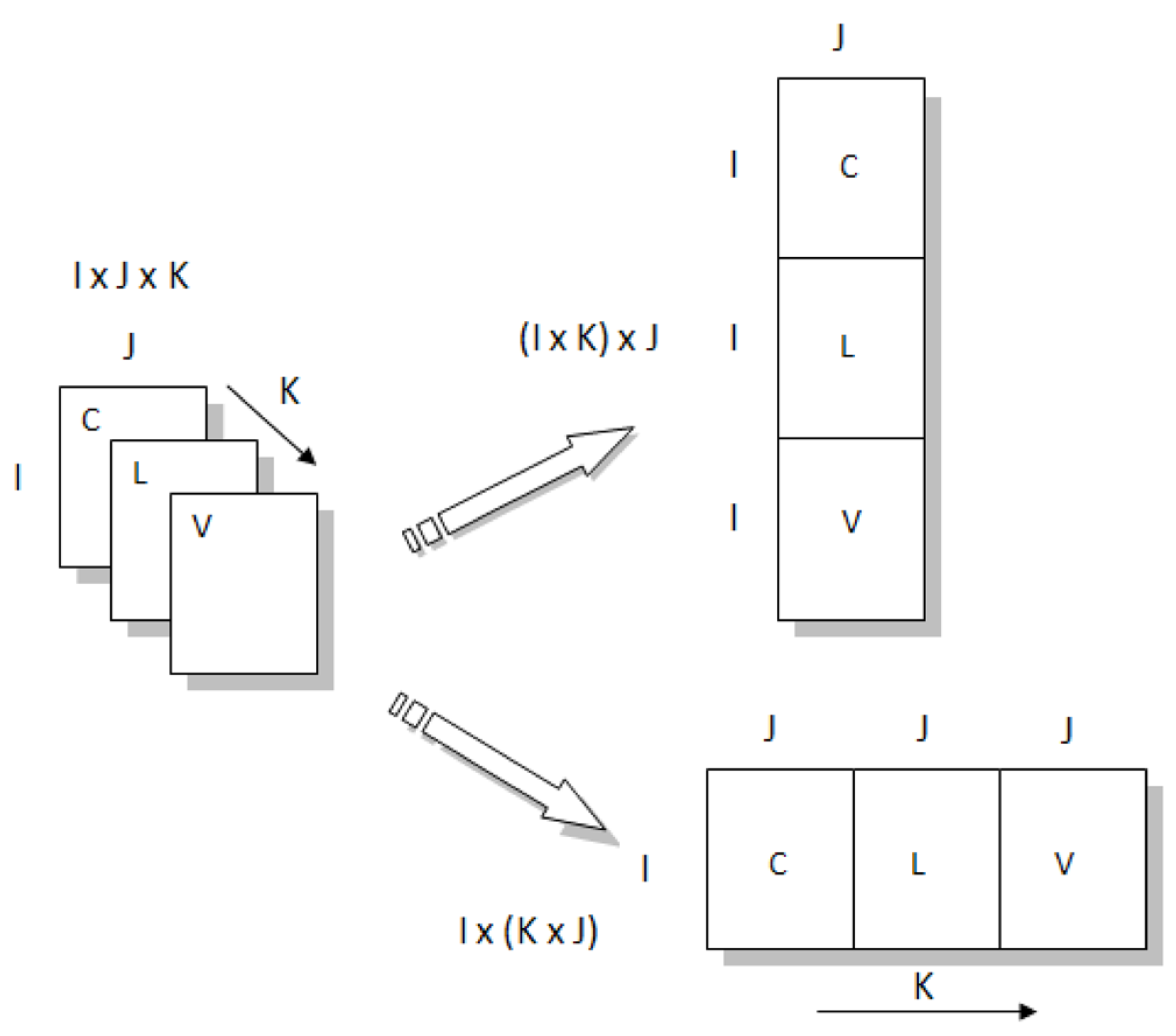
• Unfold-PCA
  As mentioned above, PCA can be also used with satisfying results when data have an intrinsically multidimensional structure, but a transformation of the array is necessary to obtain a bidimensional data matrix. This will lead to information mixing in at least one of the two dimensions of the data matrix.
  For a three-dimensional array X (I × J × K), where I represents the samples, J the variables, and K the conditions (in this article I = time, J = chemical variables, and K = sampling sites), different unfolding schemes could be applied, depending on the modeling purpose (Figure 3). Two strategies were considered in this article:

  -

  mixing the information of samples and conditions in a matrix (I × K) × J, with the goal of investigating sample variations in time;

  -

  mixing the information of samples and variables in a matrix I × (K × J), to study the relationships between the variables and the average changes of the investigated sites in time.

2.2.3. Multidimensional Modeling: Tucker3

The Tucker3 method, also called multi-way PCA, is the extension of the PCA in the case of data with three or more dimensions. Each dimension is defined as a “mode” of the calculation. The algorithm took its name from the psychometrician Ledyard R. Tucker who proposed it in 1966 [22]. Several improvements were performed since then [8,23,24]. In this article, the authors decided to arrange the data in four dimensional arrays.

For a four-way data matrix the model calculates the decomposition of the original data X (I × J × K × L) in four loadings matrices A (I × S), B (J × M), C (K × N), D (L × P), one core matrix, Z (S × M × N × P), and one error matrix, E (I × J × K × L), as expressed in:

$$x_{ijkl}={\displaystyle \sum }_{s=1}^S{\displaystyle \sum }_{m=1}^M{\displaystyle \sum }_{n=1}^N{\displaystyle \sum }_{p=1}^P{a}_{is}{b}_{jm}{c}_{kn}{d}_{lp}{z}_{smnp}+e_{ijkl}$$

The loadings matrices A, B, C, and D represent the four modes (in PCA we have only two matrices that correspond to two modes: the score matrix and the loading matrix) whereas S, M, N, and P represent the number of extracted factors from each of the four modes (note that when dealing with multiway modeling the new extracted variables are called “factors” instead of “Principal Components”). While in the PCA the number of components to be interpreted is the same in both score plot and loading plot, in Tucker3 the number of factors could be different for each mode. Any component of one mode can be linked to any component of the other modes: Tucker3 model could be considered a flexible model in this sense. The study of the sign in the core matrix (Z) is required for the correct interpretation of information. The core matrix Z (S × M × N × P) describes the relationship between the different modes: it allows the signs of the factors, and consequently the axis orientation in the plots of each mode, to be established.

The error matrix E (I × J × K × L) includes the random variation.

2.3. Experimental

Principal Component Analysis and Unfold-PCA were calculated with the software The Unscrambler 9.8 (CAMO). Multiway modeling was carried out in N-way toolbox [24] running under Matlab environment (The MathWorks Inc., Palo Alto, CA, USA).

Dealing with Missing Data

Different kinds of non-numerical values were present in the original data matrix (hourly averages × number of variables × number of sites): (1) instrument error codes (problems occurred with the analyzers); (2) values under the analytical method detection limit (LOD) which are called censored data. The censored data (around 2%) were substituted with LOD/10 values [25].

Matrices used for the unfolded-PCA method resulting in missing values for up to 7% of the data: PCA can successfully manage such a low percentage.

Matrices used for the N-Way method had missing values for up to 12% of the data. The Tucker3 algorithm [24] processes missing elements via an iterative approach called expectation maximization (EM) formulated by Dempster et al. [26]. The kind of approach applied to the Tucker3 model has also been presented by Walczak and Massart [27,28]. In the first step of this procedure the missing elements are replaced by one third of the mean row-wise and one third of the mean column-wise. During the following consecutive steps of the alternating least squares algorithm they are replaced with their predicted values, based on the currently constructed model. The calculation continues until the model residuals minimization is obtained, meaning up to the point in which there is no significant difference in the estimated missing values and the convergence of the algorithm is reached.

3. Results and Discussion

Two-way and multiway modeling interpretation is obtained basically through the evaluation of bidimensional plots. It is worthwhile to remind that in the Tucker3 model the plots axis directions depend on the sign of the correspondent core matrix element. As the bidimensional modeling is well known and widely used in atmospheric sciences, in this article the Tucker3 model interpretation will be clarified in a more detailed way.

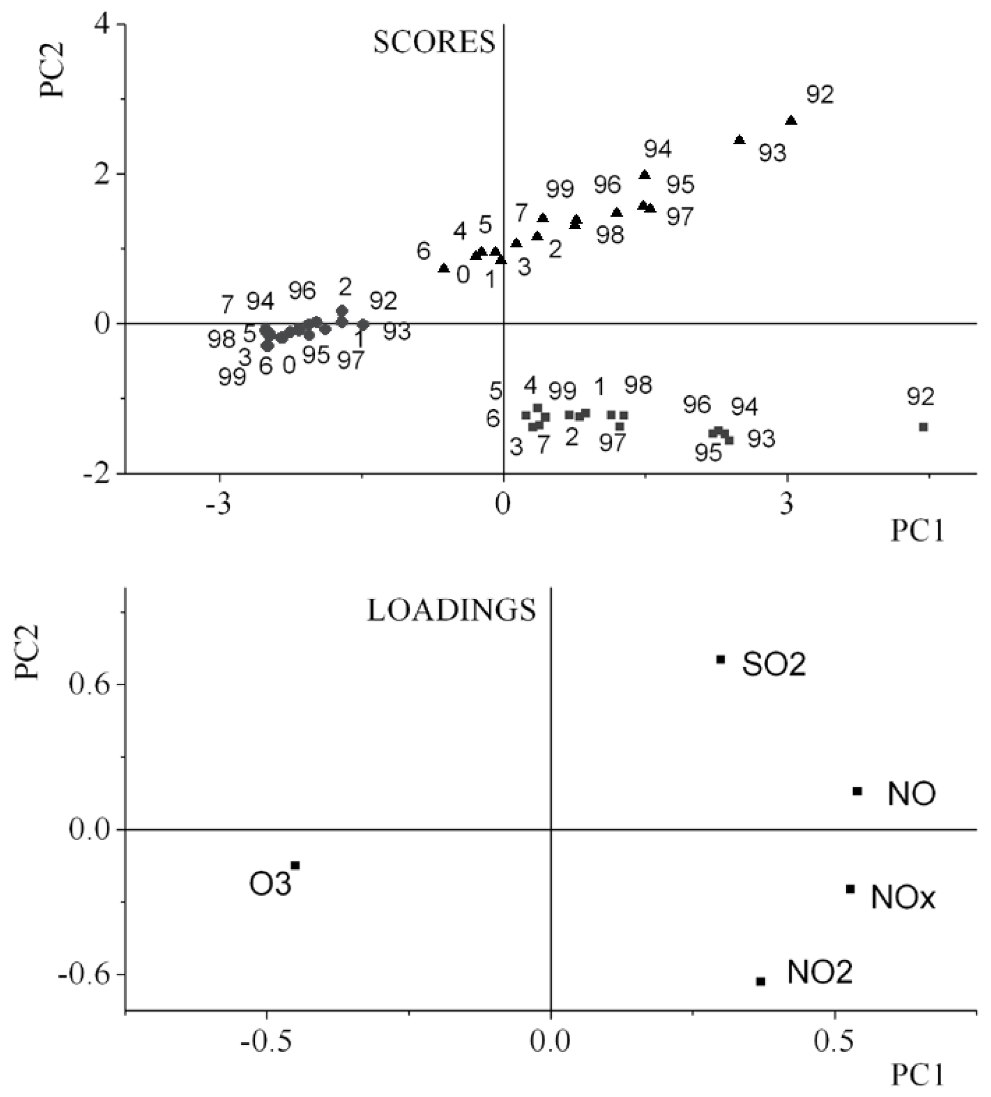
3.1. Unfold-Principal Component Analysis

The unfold-PCA calculation was performed firstly on the 2D array with the 16 yearly average values (1992–2007) for the three sites in the rows and5 variables in the columns. Autoscaling was performed on the unfolded matrix. The aim of this model was the comprehension of the differences between the sites with respect to the investigated variables and their changes in time. A score and loading plot are shown in Figure 4.

The first PC explained 62% of the total variance, the second one explained 28%. In the loading plot, PC1 showed the difference between a primary pollutant located along positive values of the axis and O₃, which had a negative value. The second component, instead, differentiated the primary pollutants.

Three sample groups emerged in the score plot. The first component differentiated the samples collected in the two urban sites (positive values) from the rural one (negative scores). PC2 differentiated Como (labelled as squares in the plot) and Lecco (labelled as triangles in the plot) samples. A pattern could be also detected: while all the Varenna samples were positioned in a small graph area, Como and Lecco samples were found from positive PC1 values (earliest sampling years) to values closer to the zero (more recent years). It is worthwhile to note that the two trends had a different direction in the PCs space.

Some interesting conclusions arose from this model. Varenna had higher O₃ values in comparison to the other two sites. On the other hand, Como was characterized by higher values of NO₂ and Lecco showed higher values of SO₂. During the chosen period, the primary pollutants reduction can be observed in the two urban sites, while the environmental condition of Varenna remained more stable (average yearly data are available in Supplementary Materials, Table S1).

A subsequent unfold-PCA was performed on the autoscaled array with 16 yearly average values in the rows and 5 variables for the 3 sites in the columns. The aim of this calculation was the study of the relationship between variables according to their environmental behavior and their variation in time. The results are shown in Figure 5.

The first two PCs retained 76% of the total variance (PC1 62%, PC2 14%—subsequent PCs did not add any valuable information).

In the loading plot the first component accounted for the information concerning primary pollutants in the three sites: these variables appeared to be highly correlated especially for the Como and Lecco sites. PC2 was mainly influenced by O₃ (the secondary pollutant) values.

In this case, the model highlighted the correlation between different variables according to their environmental source (it is worthwhile to note that their position in the plot was quite different in comparison to the loading plot obtained by the previously described PCA model).

In the score plot the samples were found along the PC1 direction: they went from 1992 (negative values) to the more recent years that showed positive score values (years starting from 2000 occupied a small area on the plot). From the model arose an average primary pollutants reduction from 1992 (the most polluted situation) to 2000 and a successive stabilization. O₃ levels (averaged on the three sites) did not show significant changes.

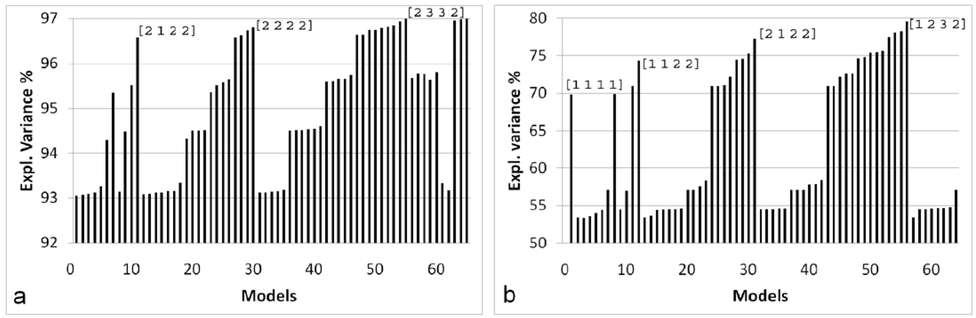
3.2. Four-Way Tucker3 Model

The first multiway model was calculated arranging the data set in a four-way array 365 days × 5 parameters × 16 years × 3 sites. Logarithmic transformation and J-scaling (scaling within variables mode) were applied prior to modeling. The aim of this model was to investigate: (1) the trends of the pollutants in the period 1992–2007; (2) the variability of the pollutants throughout the year; (3) the differences between the three considered sites.

The optimal model complexity given a proper explained variance (in other words, the optimum number of factors for each mode to be considered), was detected through the scree plot evaluation [29,30] in which models against explained variance % are reported (see Figure 6). The scree plot was realized by starting the calculation from the model with one factor in each mode [1,1,1,1] until the model [5,5,5,3]. The optimal model showed the better compromise between the smaller number of factors in each mode and the higher percentage of the data variance—several models were taken into account when selecting it.

The decomposition model [2,1,2,2] that explained 96.5% of the total data variance was chosen for further investigation (Figure 6a). All of the four modes but one were described by two factors, the second mode only needed one factor. The first mode (A) contained information concerning the days of the year, the second mode (B) contained the correlation between the parameters, and the third (C) and the fourth (D) models contained the differences between the years and the sites, respectively.

The most important core elements of Z (the core array) were [1,1,1,1], [2,1,1,2], and [1,1,2,2] that respectively explained 64.5%, 21.1%, and 6.2% of the core variance, which accounted for 91.8% of the total core variance. The loading plots for the different modes are shown in Figure 7.

The first important core element [1,1,1,1] explained 64.5% of the core variance and carried the information about the interaction between all the first factors in each mode (A1, B1, C1, D1). The sign of this core element was (−). Along the first axis of mode A (days) and mode C (years), all the loadings showed positive values, therefore the sign of the core element was determined by the signs of modes B (variables) and D (sites). B1 was mainly related to the variation of variables NO, NO₂, NO_x, and SO₂, which were highly correlated between them at negative loading values. O₃ showed a positive loading value. This axis discriminated between the primary pollutants and the secondary one. D1 differentiated the rural town, Varenna (V) from the two industrialized and populated cities, Como (C) and Lecco (L): Varenna had a negative loading value while Como and Lecco both had similar positive loading values. The negative sign of the core element could be explained through the interaction between high negative loading of B1 (variables) and high positive loading of D1 (sites) or vice-versa (mode A and C show all positive loadings). Thus, it could be pointed out that, on average, the concentration values of the primary pollutants reached higher levels in Como and Lecco sites and that, on the other hand, Varenna was characterized by higher levels of O₃. This consideration was notable for all the days in all the years.

The second important core element [2,1,1,2] explained 21.1% of the core variance and reflected the second factor in the first and fourth modes and the first factor in the second and third mode (A2, B1, C1, D2). A trend in the sample positions arose along A2 despite the overlapping due to the great number of samples (days). Samples were located from negative to positive values according to the season variability: winter and autumn days (labelled in black and dark gray in the plot) had negative values whereas spring and summer samples (labelled in gray and light gray in the plot) were placed at positive values. B1 distinguished between primary pollutants and O₃, as already mentioned, while all the years showed positive values on C1. Along D2 all the loadings showed negative values; no differences between the sites arose from this factor. O₃ levels (positive loading on B1) increased during spring and summer days while the primary pollutants highest values were recorded in the cold seasons.

The third important core element [1,1,2,2] had a positive sign and explained 6.2% of the core variance, it carried the information about the interaction between factors A1, B1, C2, and D2. C2 showed a trend from the first investigated years (positive values) to the more recent ones that showed negative values. The other factors have already been explained above. The third core element therefore showed the primary pollutants decreasing (as previously described by unfold-PCA models).

The second Tucker3 model presented in this article was built to study the differences between the weekly days (average values on a weekly base − Monday ÷ Sunday). The matrix was arranged into a four-way array as 7 days of the week × 5 parameters × 834 weeks × 3 sites. Logarithmic transformation and J-scaling were applied prior to modeling.

The decomposition model with complexity [2,1,2,2] (77.3% of the total data information) was chosen (Figure 6b). The most important core elements of Z were [1,1,1,1], [1,1,2,2], and [2,1,1,2] (66.8%, 31.4%, and 1.8%, respectively) with negative element signs for the first two factors and positive for the third. The loading plots for different modes are shown in Figure 8.

The first mode (A) described the difference between the days of the week, the second mode (B) described the correlation between the parameters, the third mode (C) described the difference between the weeks, and the fourth one (D) the difference between the sites.

The first important core element [1,1,1,1] explained the interaction between the first factor (A1, B1, C1, D1) in each mode. The sign of this core element was (−). Along the first axis of mode A (days) all loadings showed positive values; there were no differences between the days of the week. B1 showed a clear separation between O₃, with a positive loading value, and NO, NO₂, NO_x, and SO₂, with negative loading values. Along C1 all loadings showed positive values. D1 showed the difference between Varenna (V) at negative loading values and the other two sites Como (C) and Lecco (L) with similar positive loading values. The sign of the core element therefore depended on the interaction between high negative loadings of B1 (variables) and high positive loadings of D1 (sites), or vice-versa (mode A and C show all positive loadings). The core element [1,1,1,1] showed that Como and Lecco were characterized by a higher level of primary pollutants while Varenna showed a higher level of O₃ in all the weekdays for all the weeks. The second important core element, [1,1,2,2], accounted for 31.4% of the core variance and explained the interactions between the factors (A1, B1, C2, D2). The core element sign was (−). A1 and B1 have already been previously discussed. It is worthwhile to notice that along C2 positive values during winter weeks change into negative values in summer weeks. All the three sites had positive values along D2, but Como and Lecco showed higher values than Varenna. The sign of the second important core element depended on the interaction between high negative loadings of B1 (variables) and high positive loadings of C2 (weeks), or vice-versa, considering that mode A1 and D2 showed all positive loadings. Therefore, the core element [1,1,2,2] showed a higher concentration of primary pollutants (NO, NO₂, NO_x, and SO₂) in winter and autumn, whereas the secondary pollutant (O₃) was higher in summer and spring for all the weekdays and for all the sites. Again, Como and Lecco showed higher values of primary pollutants.

The third important core element [2,1,1,2] accounted for 1.8% of the core variance and explained the interaction between the factors (A2, B1, C1, D2). The core element sign was (+). A2 showed the difference between weekends (Saturday and Sunday) with positive axis values and working-days (Monday to Friday) with negative values. B1 showed positive values of O₃ and negative values for the primary pollutants, while C1 and D2 showed positive values respectively for the weeks and the sites. Therefore, the core element [2,1,1,2] showed higher concentrations of primary pollutants (NO, NO₂, NO_x and SO₂) on working-days and a higher concentration of the secondary pollutant (O₃) during weekends for all the weeks and all the sites.

From this model a difference between weekends and working-days arose. This model showed the difference between Varenna and the other two cities and confirmed ARPA site classifications as expected like the previous computed model. Moreover, cold seasons (winter and autumn) showed higher primary pollutant concentrations and O₃ reached the maximum values in the warm seasons (summer and spring), as already shown in the previous model.

4. Conclusions

Several conclusions can be drawn both from the modeling and the environmental points of view.

Both PCA and Tucker3 models could be classified as projection methods: they allow researchers to summarize the information hidden in multidimensional data onto lower dimensional subspaces with minimal loss of variance. They capture the structure in the data and return it through bidimensional graphs that give qualitative information.

The information concerning the average change in the sites during a certain time period (with respect to the considered variables) and the variables correlations, according to their environmental behavior, was obtained by the unfold-PCA strategy: two models were calculated (some sources of variability were mixed in one of the two dimensions of the data matrix) and a few numbers of bidimensional graphs were commented.

The multiway models gave all these forms of information from a single calculation taking into account the distinction between polluted and unpolluted sites, the correlation between variables according to the environmental behavior, the average change during the considered time period, and the information concerning temporal cycles, (such as the seasonal and the weekly cycles). On the other hand, both the calculation and the results interpretation could be considered a little more difficult or unusual when using the Tucker3 model, considering that it is not as common as PCA and scientists are not as used to using it. It is worthwhile to note that depending on the desired goals the data could have been arranged in a variety of different manners. Multiway modeling is a really powerful tool from this point of view because it allows researchers to distinguish and separately analyze all the sources of variation assigning one mode of the array to each of the others. Another important point arose from this project: results obtained by both strategies (two-way and multiway) were in agreement, in that correct data entry and data preparation (preprocessing and pretreatment) followed by a proper interpretation of the calculation results led to correct conclusions both from the modeling and, in this case, from the environmental points of view as well.

Concerning the case study, the investigated tropospheric data were fully explored. A characterization over time of Lake Como Area troposphere, with respect to the considered pollutants, was obtained for the first time in our knowledge through this modeling. The models highlighted a distinction between the two “hot spot” (US EPA, 2006) stations of Como and Lecco and the Varenna rural town, and it confirmed the ARPA classification that assigned Varenna into a rural site category. A pollution reduction trend and an observed change in the type of contaminants during the investigated years emerged from the modeling, as mentioned also by other authors [31] who have registered a variation in the pollutants typology in Lake Como Area. Reduction of the primary pollutants could be related to the introduction of new vehicle technologies that had to comply with increasingly stringent EU emission standards, and, as far as SO₂ is concerned, to the reduction of sulphur content in the fuel, imposed by the European directive [31]. The seasonal cycle with the O₃ peak in the summer was shown as expected. This could be explained considering the well-known direct correlation between O₃ concentration values, solar radiation, and temperature [32,33,34,35]. Moreover, a weekly cycle with the reduction of pollutants during the weekends was described, perhaps related to the smaller number of vehicles circulating during the non-working days. To obtain a complete description of the environment under study other variables could be studied (e.g., meteorological parameters, wind analysis, etc.) and this will be the object of a future investigation that will be focused on considering environmental aspects.

Beyond considerations surrounding the chosen case study, the chemometric methods and especially the multiway modeling that were successfully employed in this project could be applied to more complex data matrices (e.g., more sampling points, analytes, conditions, etc.), without any further complication in the interpretation of the results.

This article would like to offer a powerful alternative to handle the huge data set coming from atmospheric studies. It is worthwhile to note that the proposed methods could add value to historical databases as well, with the aim of detecting and/or preventing environmental problems in an easy and swift manner.

References

- Brunekreef, B.; Holgate, S.T. Air pollution and health. Lancet 2002, 360, 1233–1242. [Google Scholar] [CrossRef]
- Henry, R.C.; Hidy, G.M. Multivariate analysis of particulate sulfate and other air quality variables by principal component analysis—Part I: Annual data from Los Angeles and New York. Atmos. Environ. 1979, 13, 1581–1596. [Google Scholar] [CrossRef]
- Henry, R.C.; Hidy, G.M. Multivariate analysis of particulate sulfate and other air quality variables by principal component analysis—Part II: Salt Lake City, Utah and St. Louis, Missuri. Atmos. Environ. 1979, 13, 1581–1596. [Google Scholar] [CrossRef]
- Han, Y.M.; Du, P.X.; Cao, J.J.; Posmentier, E.S. Multivariate analysis of heavy metal contamination in urban dusts of Xi’an, Central China. Sci. Total Environ. 2006, 355, 176–186. [Google Scholar]
- Pires, J.C.M.; Pereira, M.C.; Alvim-Ferraz, M.C.M.; Martins, F.G. Identification of redundant air quality measurements through the use of principal component analysis. Atmos. Environ. 2009, 43, 3837–3842. [Google Scholar] [CrossRef]
- Yonemura, S.; Kawashima, S.; Matsueda, H.; Sawa, Y.; Inoue, S.; Tanimoto, H. Temporal variations in ozone concentrations derived from PCA. Theor. Appl. Climatol. 2008, 92, 47–58. [Google Scholar] [CrossRef]
- Merino, A.; Wu, X.; Gascón, E.; Berthet, C.; García-Ortega, E.; Dessens, J. Hailstorms in southwestern France: Incidence and atmospheric characterization. Atmos. Res. 2014, 140–141, 61–75. [Google Scholar] [CrossRef]
- Leardi, R.; Armanino, C.; Lanteri, S.; Alberotanza, L. Three-mode principal component analysis of monitoring data from Venice lagoon. J. Chemometr. 2000, 14, 187–195. [Google Scholar] [CrossRef]
- Barbieri, P.; Adami, G.; Piselli, P.; Gemiti, F.; Reisenhofer, E. A three-way principal factor analysis for assessing the time variability of freshwaters related to a municipal water supply. Chemom. Intell. Lab. Syst. 2002, 62, 89–100. [Google Scholar] [CrossRef]
- Stanimirova, I.; Kita, A.; Malkowski, E.; John, E.; Walczak, B. Nway exploration of environmental data obtained from sequential extraction procedure. Chemom. Intell. Lab. Syst. 2009, 96, 203–209. [Google Scholar] [CrossRef]
- Engle, M.A.; Gallo, M.; Schroeder, K.T.; Geboy, N.J.; Zupancic, J.W. Three-way compositional analysis of water quality monitoring data. Environ. Ecol. Stat. 2014, 21, 565–581. [Google Scholar] [CrossRef]
- Giussani, B.; Monticelli, D.; Gambillara, R.; Pozzi, A.; Dossi, C. Three-way principal component analysis of chemical data from Lake Como watershed. Microchem. J. 2008, 88, 160–166. [Google Scholar] [CrossRef]
- Sillmann, S. The relation between ozone, NOx and hydrocarbons in urban and polluted rural environments. Atmos. Environ. 1999, 33, 1821–1845. [Google Scholar] [CrossRef]
- Jenkin, M.E.; Clemitshaw, K.C. Ozone and other secondary photochemical pollutants: Chemical processes governing their formation in the planetary boundary layer. Atmos. Environ. 2000, 34, 2499–2527. [Google Scholar] [CrossRef]
- Zeng, Y.; Hopke, P.K. Methodological study applying three-mode factor analysis to three-way chemical data sets. Chemom. Intell. Lab. Syst. 1990, 7, 237–250. [Google Scholar] [CrossRef]
- Malik, A.; De Juan, A.; Tauler, R. Multivariate curve resolution: A different way to examine chemical data. In 40 Years of Chemometrics—From Bruce Kowalski to the Future; ACS Symposium Series: Washington, DC, USA, 2015; Volume 1199, pp. 95–128. [Google Scholar]
- Bro, R. PARAFAC. Tutorial and applications. Chemom. Intell. Lab. Syst. 1997, 38, 149–171. [Google Scholar] [CrossRef]
- De Noord, O.E. The influence of data preprocessing on the robustness and parsimony of multivariate calibration models. Chemom. Intell. Lab. Syst. 1994, 23, 65–70. [Google Scholar] [CrossRef]
- Kroonenberg, P.M. Three-Mode Principal Component Analysis; DSWO Press: Leiden, The Netherlands, 1983. [Google Scholar]
- Wold, S.; Esbensen, K.; Geladi, P. Principal component analysis. Chemom. Intell. Lab. Syst. 1987, 2, 37–52. [Google Scholar] [CrossRef]
- Brereton, R. Applied Chemometrics for Scientists; Wiley: Hoboken, NJ, USA, 2007. [Google Scholar]
- Tucker, L.R. Some mathematical notes on three-mode factor analysis. Psychometrika 1966, 31, 279–311. [Google Scholar] [CrossRef] [PubMed]
- Andersson, C.A.; Bro, R. Improving the speed of multi-way algorithms: Part I. Tucker3. Chemom. Intell. Lab. Syst. 1998, 42, 93–103. [Google Scholar] [CrossRef]
- Andersson, C.A.; Bro, R. The N-way toolbox for MATLAB. Chemom. Intell. Lab. Syst. 2000, 52, 1–4. [Google Scholar] [CrossRef]
- Alier, M.; Felipe-Sotelo, M.; Hernàndez, I.; Tauler, R. Variation patterns of nitric oxide in Catalonia during the period from 2001 to 2006 using multivariate data analysis methods. Anal. Chim. Acta 2009, 642, 77–88. [Google Scholar] [CrossRef] [PubMed]
- Dempster, A.P.; Laird, N.M.; Rubin, D.B. Maximum likelihood for incomplete data via the EM algorithm. J. R. Stat. Soc. B 1977, 39, 1–38. [Google Scholar]
- Walczak, B.; Massart, D.L. Dealing with missing data: Part I. Chemom. Intell. Lab. Syst. 2001, 58, 15–27. [Google Scholar] [CrossRef]
- Walczak, B.; Massart, D.L. Dealing with missing data: Part II. Chemom. Intell. Lab. Syst. 2001, 58, 29–42. [Google Scholar] [CrossRef]
- Zhang, L.; Marron, J.S.; Shen, H.P.; Zhu, Z. Singular value decomposition and its visualization. J. Comput. Graph. Stat. 2007, 16, 833–854. [Google Scholar] [CrossRef]
- Zhu, M.; Ghodsi, A. Automatic dimensionality selection from the scree plot via the use of profile likelihood. Comput. Stat. Data Anal. 2006, 51, 918–930. [Google Scholar] [CrossRef]
- Caserini, S.; Giuliano, M.; Pastorello, C. Traffic emission scenarios in Lombardy region in 1998–2015. Sci. Total Environ. 2008, 389, 453–465. [Google Scholar] [CrossRef] [PubMed]
- Liu, C.M.; Huang, C.Y.; Shield, S.L.; Wu, C.C. Important meteorological parameters for ozone episodes experienced in the Taipei basin. Atmos. Environ. 1994, 28, 159–173. [Google Scholar] [CrossRef]
- Atkinson, R. Atmospheric chemistry of VOCs and NOx. Atmos. Environ. 2000, 34, 2063–2101. [Google Scholar] [CrossRef]
- Chang, S.C.; Lee, C.T. Evaluation of trend of air quality in Taipei, Taiwan from 1994 to 2003. Environ. Monit. Assess. 2007, 127, 87–96. [Google Scholar] [CrossRef] [PubMed]
- Chang, S.C.; Lee, C.T. Secondary aerosol formation through photochemical reactions estimated by using air quality monitoring data in Taipei City from 1994 to 2003. Atmos. Environ. 2007, 41, 4002–4017. [Google Scholar] [CrossRef]
© 2016 by the authors; licensee MDPI, Basel, Switzerland. This article is an open access article distributed under the terms and conditions of the Creative Commons Attribution (CC-BY) license (http://creativecommons.org/licenses/by/4.0/).
Share and Cite
Giussani, B.; Roncoroni, S.; Recchia, S.; Pozzi, A. Bidimensional and Multidimensional Principal Component Analysis in Long Term Atmospheric Monitoring. Atmosphere 2016, 7, 155. https://doi.org/10.3390/atmos7120155
Giussani B, Roncoroni S, Recchia S, Pozzi A. Bidimensional and Multidimensional Principal Component Analysis in Long Term Atmospheric Monitoring. Atmosphere. 2016; 7(12):155. https://doi.org/10.3390/atmos7120155
Chicago/Turabian StyleGiussani, Barbara, Simone Roncoroni, Sandro Recchia, and Andrea Pozzi. 2016. "Bidimensional and Multidimensional Principal Component Analysis in Long Term Atmospheric Monitoring" Atmosphere 7, no. 12: 155. https://doi.org/10.3390/atmos7120155
APA StyleGiussani, B., Roncoroni, S., Recchia, S., & Pozzi, A. (2016). Bidimensional and Multidimensional Principal Component Analysis in Long Term Atmospheric Monitoring. Atmosphere, 7(12), 155. https://doi.org/10.3390/atmos7120155