Article

Measurement of Ozone Concentration on the Elevation Gradient of a Low Hill by a Semiconductor-Based Portable Monitor

Faculty of Agriculture, Ehime University, 3-5-7 Tarumi, Matsuyama, Ehime 7908566, Japan
Atmosphere 2015, 6(7), 928-941; https://doi.org/10.3390/atmos6070928
Submission received: 26 May 2015 / Revised: 6 July 2015 / Accepted: 8 July 2015 / Published: 14 July 2015

Abstract

:
Ozone concentration has a complex distribution in mountain areas, but the low spatial density of high elevation monitoring stations has limited our understanding of ozone behavior. To achieve high spatial density, mobile measurement was carried out using a portable ozone monitor based on a semiconductor sensor. On the elevation gradient of a relatively low hill (273 m above seal level) in Matsuyama, Japan, 66 walking measurements were conducted in the pre-dawn hours of the winter in 2012 and 2013. The ozone concentration at the top of the hill was positively correlated with the daily maximum concentration on the plain on the previous day. The difference in ozone concentration between the top and bottom of the hill was found to increase with increasing vertical temperature difference. The measurement method established in this study provides a low-cost alternative to grasp the distribution of ozone in mountain areas.

1. Introduction

Tropospheric ozone has deteriorating effects on forest trees (e.g., [1] for a review) in addition to other negative impacts, such as worsening symptoms of human respiratory diseases [2] and acting as a green-house gas [3]. The observed decline of mountain forests and the increasing trend of tropospheric ozone in the Northern Hemisphere [4] have prompted the installation of monitoring stations of ozone and other relevant species in high-elevation mountains [5,6,7,8]. Such stations have revealed various aspects of the vertical structure of ozone concentration, and we have a fairly good understanding of the broad-scale behaviors of tropospheric ozone.
At smaller scales, it has been observed that the decline of forest trees occurs non-uniformly over mountains, often restricted to certain areas [9]. Furthermore, previous studies [6,10] noted a different dependence of ozone concentration on elevation along different transects in the same regions. Therefore, for proper understanding of the behavior in mountains, ozone concentration needs to be measured at a higher spatial density. However, the cost of the installation and maintenance of high-elevation stations is much higher than that of low-elevation stations. To overcome the cost problem, passive samplers have often been employed [11], but the inevitable low temporal resolution has made it difficult to relate the concentration variation to atmospheric processes involving ozone. At present, we do not know the spatial distribution and temporal variation of ozone at resolutions that are sufficient for identifying the cause of forest decline, which can be caused by other factors, such as feeding damage by insects or deer, or water stress.
The vertical structure of ozone concentration is also important for understanding the life cycle of ozone in urban areas. Monitoring on towers [12] and measurement using tethered balloons [13,14] are standard methods to obtain vertical profiles. Transect measurements along mountain slopes is also an efficient way to grasp the vertical structure at high temporal resolution for a long time [15]. These methods provide high-quality data at strategic locations, but the high cost of equipment and the difficulty of finding adequate sites limit the application to arbitrary places.
Recently, portable ozone monitors have been developed that operate on low electric voltages [16]. The portability enables a spatially-dense measurement and helps identify the locations where ozone concentration changes substantially. Furthermore, the vertical profiles of ozone concentration can be obtained at a much lower cost than by the conventional methods. This paper describes an application of a battery-powered portable ozone monitor to a relatively low mountain and demonstrates the feasibility of using such devices for spatially-dense monitoring in mountain areas.

2. Observation

2.1. Site

The observation site is Awajigatou (the Awaji pass by direct translation from Japanese) on the eastern edge of the Dogo plain in Matsuyama city, Japan (Figure 1). Matsuyama is the capital of the Ehime prefecture on the Shikoku island in the western part of Japan. Matsuyama has a population of about 500 thousand with major industries in agriculture, manufacturing, business services and tourism. There are many factories of the secondary industry mainly of chemical manufacturing in the coastal area in the west of Matsuyama. The Dogo plain, the core area of Matsuyama, is surrounded by the Seto inland sea on the west, the Takanawa mountains (∼1000 m above sea level (a.s.l.)) on the northeast and the Shikoku mountains (1000–2000 m a.s.l.) on the east to southeast. Except for scattered hills at most about 130 m, the Dogo plain is flat. This orography generates a clear diurnal alternation of sea breeze in the daytime and land breeze at night. Figure 2 shows the diurnal pattern of the wind field measured at the Matsuyama meteorological observatory (33°50.6' N, 132°46.6' E) located in the center of the Dogo plain.
Figure 1. Locations of Matsuyama city and Awajigatou (green area and red triangle, respectively, in the inset map) and the measurement route (A → G → A). The curves indicate elevation contours at 10-m intervals, with the thick ones representing 100 m and 200 m a.s.l.
Atmosphere 06 00928 g001
Figure 2. Mean diurnal variations of wind speed (WS, solid line) and wind direction (WD, dots) observed as 10-minute averages prior to the hour at Matsuyama meteorological observatory from 1 December 2012–3 March 2013.
Atmosphere 06 00928 g002
The route to the summit of Awajigatou (G in Figure 1; 33°49.9'N, 132°48.5'E, 273 m a.s.l.) is a walking trail for the maintenance of power transmission towers installed at a few hundred-meter intervals. From the bottom end (C in Figure 1), the walking trail runs beside a mandarin orchard for about 100 m (D in Figure 1), through a relatively dense canopy (∼15 m high; E in Figure 1) up to a ridge and along the ridge (F in Figure 1), with relatively short and sparse trees of 3–7 m high up to the summit (G in Figure 1). Along the ridge, there are occasionally wide openings either to the east or west. The summit area (approximately 150 m2) is mostly cleared of trees for a resting hut and a viewing deck. The width of the walking trail is about 0.6 m up to the ridge (from C–E in Figure 1) and about 1.5 m along the ridge up to the summit (from E–G in Figure 1). The surface of the walking trail is mostly bare soil with occasional rocks. The trees on Awajigatou are of a mixed variety, including red pine, oak and chestnut. The under-bush around the walking trail is mostly fern.
The path between the starting point (A in Figure 1) to the foot of Awajigatou (C in Figure 1) is a paved single-lane road that runs through a residential area, which is mostly flat, except for a small hill (B in Figure 1) about 15 m high. Cars seldom passed by during the measurements. It took a little more than an hour for the return trip between the starting point and the summit of Awajigatou. The up and down routes were walked at almost the same speed, so that the temporal rate of change of elevation became nearly symmetric (cf. Figure 6).
The height of Awajigatou is much smaller than the mountains studied by previous authors as “high-elevation” sites. Awajigatou is lower than a typical convective boundary layer of 1–2 km thick, but is comparable to the height of a typical nocturnal surface inversion. Therefore, observation at Awajigatou at night reveals the behaviors through the surface inversion up to the residual layer where the remnant of ozone exists from the previous-day convective boundary layer [17].
Figure 3. Mean diurnal behaviors of the concentrations of nitric oxide (NO, triangles), nitrogen dioxide (NO2, squares) and ozone (O3, circles) measured at the Tomihisacho ambient air monitoring station in Matsuyama city from 1 December 2012–3 March 2013.
Atmosphere 06 00928 g003
Diurnal variations of the air-pollutant concentrations measured at the Tomihisacho ambient air-monitoring station (33°49.2' N, 132°43.7' E) in the Dogo plain (averages from 1 December 2012–3 March 2013) are shown in Figure 3. Although the concentration levels are moderate, the diurnal behaviors are typical of urban areas; nitric oxide (NO) is maximal in the morning rush hour, and ozone (O3) is maximal in the late afternoon. The daily minimum of hourly average O3 occurs from 7:00–8:00 when the NO emission by the morning traffic is high, but the photochemical production of O3 is still low [18]. In winter, the nighttime level of O3 is relatively high (∼20 ppbv), because the nocturnal ozone maximum [19,20,21] associated with the persistent wind from the mountains on the east occurred frequently (see Figure 2).

2.2. Period

The observations were conducted before dawn in the winter of 2012 and 2013. The reasons for the choice of this time of day are listed below.
  • Because the thickness of surface inversion peaks before dawn, the difference in ozone concentration from the bottom to the top of Awajigatou was expected to be large.
  • Because the stomata of plants are nearly closed before dawn, the consumption of ozone inside plant bodies could be assumed negligible.
  • Because the rate of change of ozone concentration is small in the pre-dawn hours, the change of concentration level during the measurement walks could be assumed negligible.
  • Because the effect of solar radiation can be neglected, the measurement of temperature and humidity could be conducted with unshielded, bare sensors.
  • Because the wind speed is usually small, transport from distant regions could be assumed negligible.
Ozone destruction during the observation period is due to decomposition on solid surfaces, such as ground and plant bodies, and chemical reaction with NO that begins to increase around 6:00 (Figure 3). Therefore, we can concentrate on meteorological effects in interpreting the observation results.

2.3. Equipment

The moving track was recorded by a GPS logger, iBlue 747 Pro (TranSystem Inc., Hsinchu, Taiwan). Temperature was measured by a thermistor sensor with a response time of 75 s (TR-73U; Ondotori, T&D Co., Matsumoto, Japan). Relative humidity was measured by a capacitive sensor with a response time of 20 s (TR-77Ui; Ondotori, T&D Co., Matsumoto, Japan). The temperature and humidity sensors were hung at the waist level without any shelters, because the effect of solar radiation could be neglected in the pre-dawn hours. Atmospheric pressure was measured by TR-73U using a piezoresistive pressure sensor.
For the measurement of ozone concentration, the Aeroqual S500 ozone monitor (Aeroqual Ltd., Auckland, New Zealand) was used. The Aeroqual S500 draws ambient air into an enclosure in which ozone molecules, by their oxidizing tendency, modify the electrical state of the sensing material, a heated thin film of tungsten oxide. The thin film is deposited on metal electrodes, and the change in the electrical resistance is measured as a proxy to the change in ozone concentration. The measurement cycle was about 68 s, whereas the data were recorded every minute as the most recently updated values. The response time was about three sampling intervals (about 3 min) for a step increase and about a single sampling interval (about 1 min) for a step decrease. More details about the measurement principle can be found in [16].

3. Results

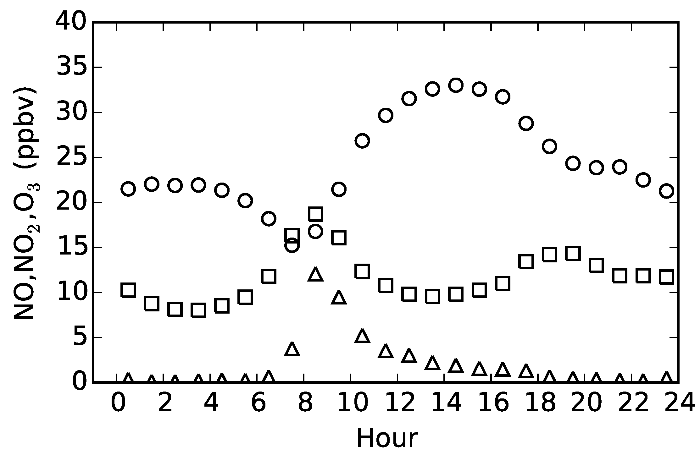
3.1. Properties of the Aeroqual S500

An important property of the Aeroqual S500 is the dependence on ambient conditions, such as temperature (T), relative humidity (ϕ) and atmospheric pressure (P). Gundel et al. [22] compared the performance of various ozone analyzers based on different principles, such as UV absorption, electrochemical concentration cell and heated metal oxide (Aeroqual S500). They used a stainless chamber to which output of an ozone generator was connected and in which the air condition was controlled arbitrarily. Assuming that an ozone analyzer based on UV absorption (API Model 400, Teledyne Technologies Inc., Thousand Oaks, CA, USA) gave the true concentration, the readings of the other devices were normalized by that of API Model 400. The dependence on P varied among different test runs, but approximately, the reading of the Aeroqual S500 became 10% smaller per pressure drop of 25 hPa. The dependence on ϕ was relatively repeatable, and the reading of the Aeroqual S500 increased by 50% per a drop of relative humidity of 40%. The dependence on T varied considerably among test runs, and there were signs of a hysteresis behavior; however, overall, the reading of the Aeroqual S500 decreased by 25% per temperature increase of 5 °C. The above-mentioned changes of P, ϕ and T are typical magnitudes experienced while climbing Awajigatou on a day with strong surface inversion. Therefore, the change in the atmospheric condition over the height of Awajigatou was expected to have competing effects of similar magnitudes on the Aeroqual S500.
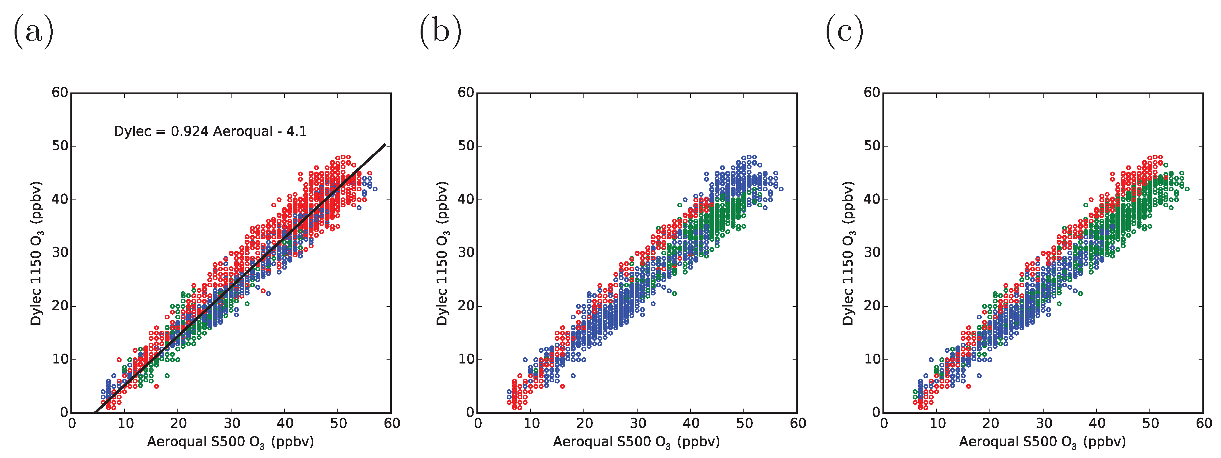
In practice, it is necessary to compare the Aeroqual S500 that was actually used for observation with a UV-based ozone analyzer in the real atmosphere. Figure 4 shows the result of such a comparison conducted on an open-air walking bridge between school buildings of the department of agriculture of Ehime University. The reference ozone analyzer was the Dylec 1150 (Dylec Co., Ltd., Ami, Japan), which had been confirmed to agree with a similar UV-based ozone analyzer used for continuous measurement at permanent air-monitoring stations in Ehime prefecture, Japan. Comparison measurements were conducted on 31 days between 7 January and 23 February 2013, each lasting for about an hour around 9:00, 12:00, 14:00 or 16:00, except for a case that continued for 24 h. The ambient T, ϕ and vapor density ( ρ v ) ranged from −1.3 to 19.8 °C, from 20% to 90% and from 2.6 to 10.5 g·m−3, respectively. Each point in Figure 4 represents a datum of the Aeroqual S500 at its sampling time (every 60 s) and that of the Dylec 1150 at its sampling time (every 12 s) closest to that of the Aeroqual S500. The marker color in Figure 4 indicates the levels of T, ϕ or ρ v . Table 1 lists the least-squares regressions for each level of T, ϕ or ρ v . Although there was a weak tendency that the reading of the Aeroqual S500 became lower as T increased or ϕ increased, linear regression resulted in rather irregular variations in the slope and y-intercept for different ranges of T or ϕ. Furthermore, the change of the reading due to changes in T or ϕ was comparable to the variation in the reading of the Aeroqual S500 for repeated measurement at a fixed point for several minutes. The cause of variability has not yet been clarified, but probable causes are fluctuations in sensor temperature and ambient wind condition. It was therefore decided that the difference in the linear regression for different T or ϕ ranges was not significant, and a calibration relation was determined using the whole measurement data.
Figure 4. Correlations between the Aeroqual S500 and the Dylec 1150 for the measurement of ambient ozone concentration. Panels (ac) show the same data with different colors depending on T (°C), ϕ (%) and ρ v (g m−3), respectively. The color definitions are: (a) T < 3 (green), 3 T < 6 (blue), 6 T (red); (b) ϕ < 50 (green), 50 ϕ < 75 (blue), 75 ϕ (red); and (c) ρ v < 3.5 (green), 3.5 ρ v < 7.0 (blue), 7.0 ρ v (red).
Atmosphere 06 00928 g004
Table 1. Least-squares regression between the Aeroqual S500 and the Dylec 1150 for different levels of T, ϕ or ρ v . R indicates Pearson’s correlation coefficient.
ItemRangeLeast-Squares RegressionR
T (°C) T < 3 ( Dylec 1150 ) = 0.788 ( AeroqualS 500 ) 1.8 0.93
3 T < 6 ( Dylec 1150 ) = 0.880 ( AeroqualS 500 ) 2.8 0.99
6 T ( Dylec 1150 ) = 0.907 ( AeroqualS 500 ) - 2.4 0.98
ϕ (%) ϕ < 50 ( Dylec 1150 ) = 0.771 ( AeroqualS 500 ) + 1.4 0.92
50 ϕ < 75 ( Dylec 1150 ) = 0.947 ( AeroqualS 500 ) - 4.9 0.98
75 ϕ ( Dylec 1150 ) = 1.059 ( AeroqualS 500 ) - 5.0 0.99
ρ v (g m−3) ρ v < 3.5 ( Dylec 1150 ) = 0.865 ( AeroqualS 500 ) 1.6 0.98
3.5 ρ v < 7.0 ( Dylec 1150 ) = 0.836 ( AeroqualS 500 ) 2.7 0.97
7.0 ρ v ( Dylec 1150 ) = 1.039 ( AeroqualS 500 ) 4.6 0.99
With Pearson’s correlation coefficient of 0.98, the linear-regression relation between the Dylec 1150 and the Aeroqual S500 became:
( Dylec 1150 ) = 0.924 ( AeroqualS 500 ) 4.1
It should be noted that similar comparison runs conducted in summer 2013 ( T = 28.7 –35.2 °C, ϕ = 45 %–74%, ρ v = 17.3 –22.4 g·m−3) resulted in a much lower reading of the Aeroqual S500 ((Dylec 1150) ≈ 1.35 × (Aeroqual S500)). Therefore, the Equation (1) is valid only during the winter observation period.
To further confirm that the measurement by Aeroqual S500 was not strongly affected by variations in T, P or ϕ along the mountain, an on-site comparison was conducted using a lightweight battery-operated UV-based ozone analyzer (Model 202, 2B Technologies, Boulder, CO, USA) that was acquired much later than the main measurement campaign. The nominal precision and response time of the 2B Model 202 are 1.5 ppbv (or 2% of reading) and 20 s, respectively. Both the Aeroqual S500 and the 2B Model 202 were carried up Awajigatou on 22, 23, 24 and 25 February 2014 (note the different year from the observations reported in much of this article). 
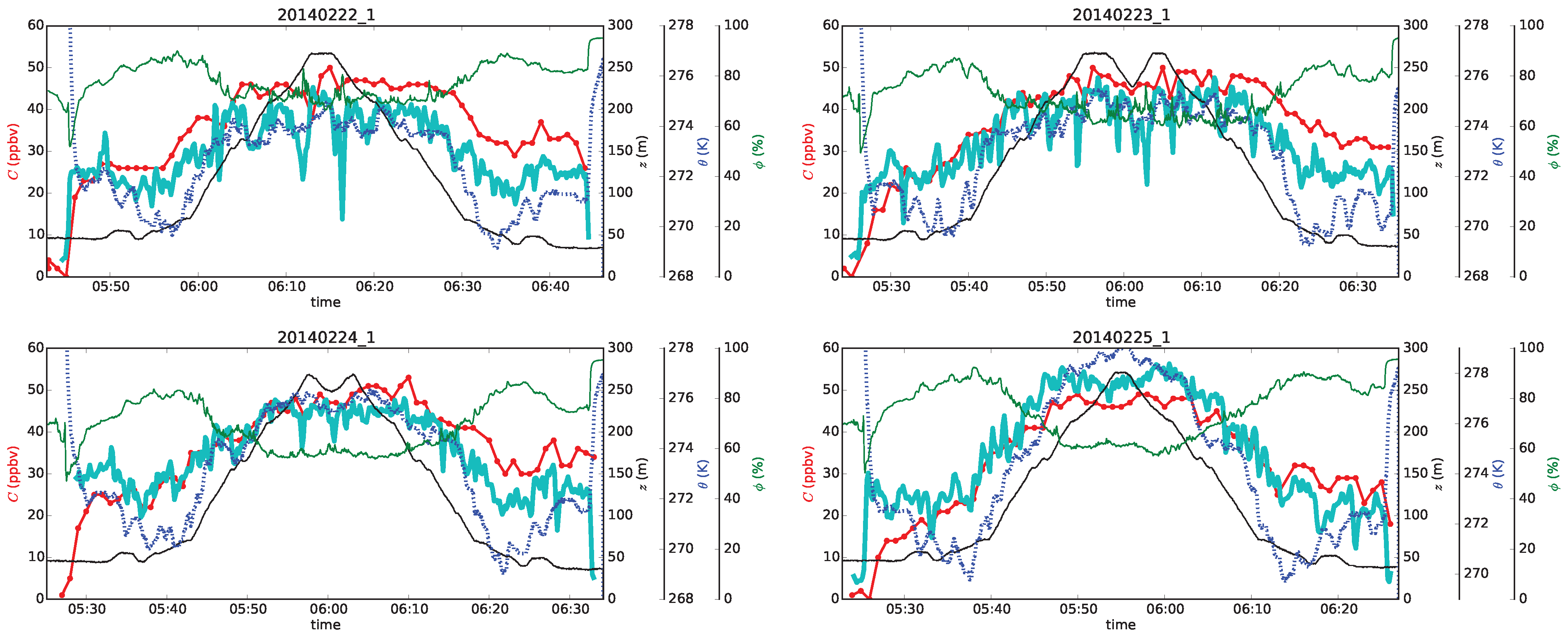
Figure 5 shows the result. In Figure 5, the data of the Aeroqual S500 were converted by Equation (1) to be equivalent to the Dylec 1150. The 2B Model 202 was confirmed to agree with the Dylec 1150. The difference between the Aeroqual S500 and the 2B Model 202 varied from day to day, but no consistent dependence on T, P or ϕ was found. The difference between the Aeroqual S500 and the 2B Model 202 was comparable to the uncertainty found for the comparison between the Aeroqual S500 and the Dylec 1150. The four measurements in Figure 5 are not used in the following analysis.
Figure 5. Comparison between the Aeroqual S500 (red) and the 2B Model 202 (thick cyan) for four Awajigatou measurements. Explanations of other quantities are given in Figure 6.
Atmosphere 06 00928 g005

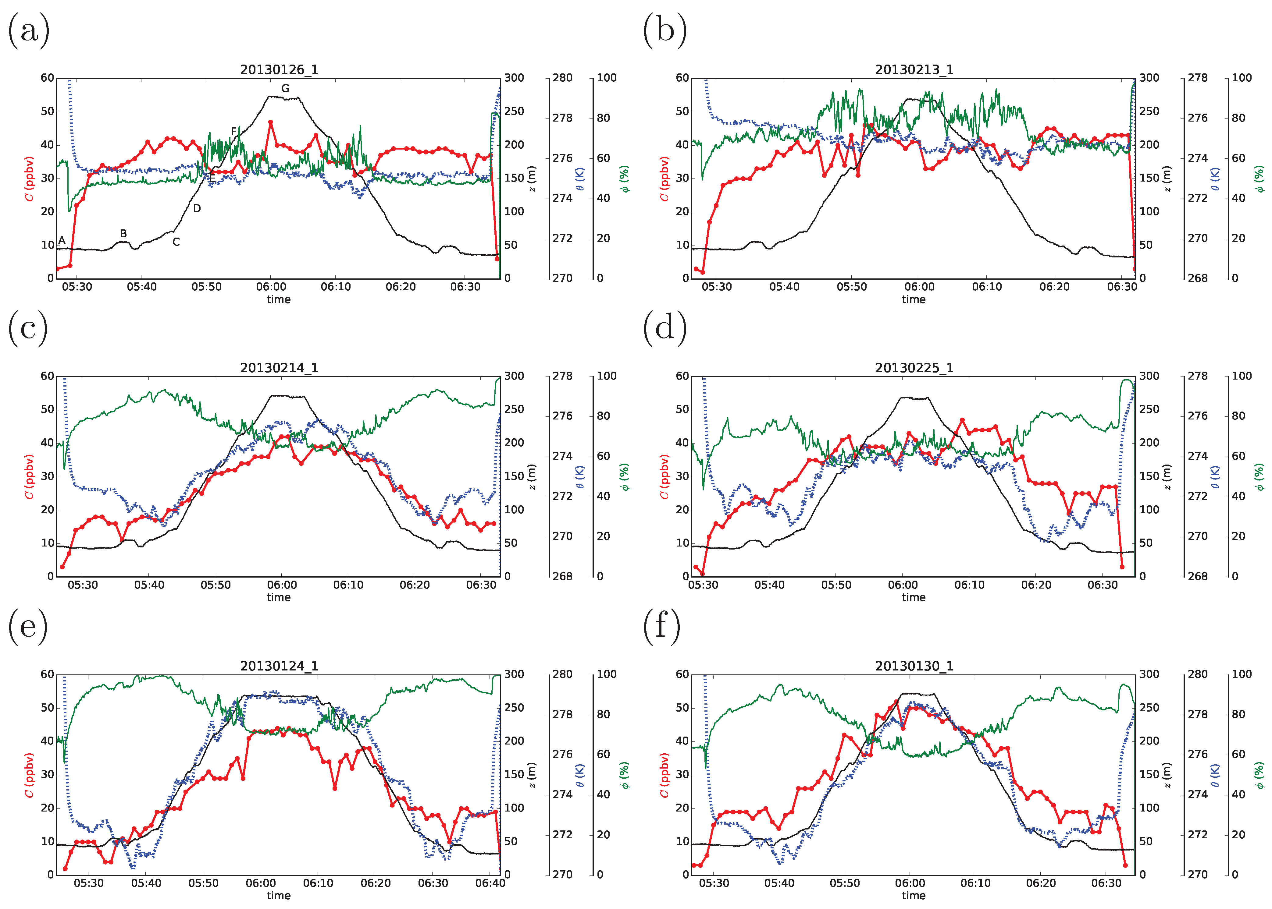
3.2. Hill Measurement Results

Representative behaviors of the potential temperature (θ), relative humidity (ϕ), elevation (z) and ozone concentration (C) are shown in Figure 6. The ozone concentration data C of the Aeroqual S500 are the result of conversion using Equation (1). The elevation z was calculated from the atmospheric pressure assuming a hydrostatic state of a column of air with a mean density between the foot and the top of Awajigatou. Along the measurement route, θ, ϕ and C changed gradually with z, but abrupt changes often occurred at canopy edges or changes of the elevation gradient. However, because such changes were not always reproducible in a few immediately-conducted repeated climbs and because the short timescale of such changes was not suited to the low time resolution of the Aeroqual S500, we focus on the difference between the bottom and top of Awajigatou in the following analysis. The short-scale variations as shown in 
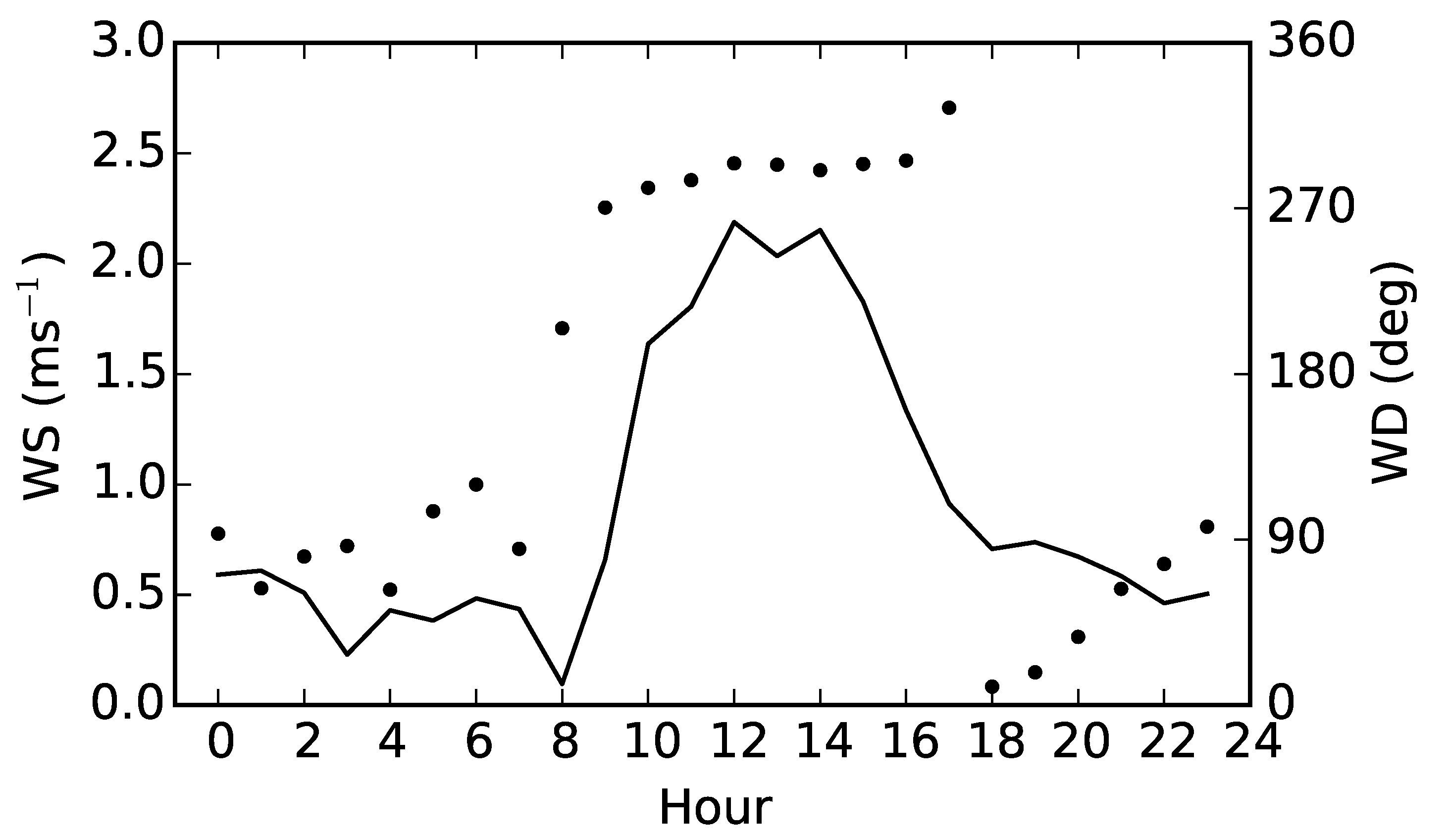
Figure 5 for the measurement results by the 2B Model 202 were considered to be caused by uphill flows along valleys. A detailed analysis with wind-field measurements will be reported in a forthcoming paper.
In the case of Figure 6a,b, the weather was cloudy and windy, and the profile of θ was flat, representing a neutral atmospheric condition. In this case, C was also generally uniform, because of the well-mixed state of a neutral boundary layer. In the case of Figure 6c–f, the weather was fine with weak wind, and θ increased with z, typical of stable atmospheric condition. The surface layer was more stable (the temperature difference between the top and the bottom was larger) in Figure 6e,f than in Figure 6c,d. In these cases, C also increased with z. As described later, the top-bottom difference of C was larger for a larger top-bottom temperature difference.
Figure 6. Representative results of Awajigatou measurements: ozone concentration C (red), elevation a.s.l. (black), potential temperature θ (blue) and relative humidity ϕ (green). Thermal stratification were neutral in (a,b), moderately stable in (c,d) and strongly stable in (e,f).
Atmosphere 06 00928 g006
A neutral condition as in Figure 6a,b was rather rare; in only 16 out of 66 observations was | Δ θ | found to be less than 2 K (corresponding to an overall Richardson number of 1.0 for a relatively large wind speed difference of 4 m s - 1 between the top and bottom of Awajigatou), where:
Δ θ = θ top - θ bottom
and θ top and θ bottom are the values of θ at the top and bottom of Awajigatou, respectively.
It should be noted that the count of Class D (neutral) in terms of the Pasquill–Gifford (PG) stability classification (see [23] for the definition adopted here) based on the measurement data of wind and cloud coverage at 6:00 at the Matsuyama meteorological observatory located in the center of the Dogo plain (Figure 1) was 36, more than twice as large as the count of cases with | Δ θ | < 2 K . 
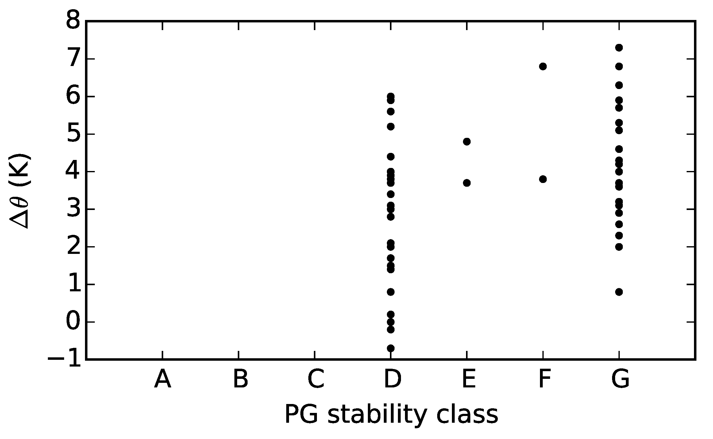
Figure 7 shows the relation between Δ θ observed at Awajigatou and the PG classes. We observe a tendency that Δ θ increases for more stable PG classes (D→E→F→G), but the variation of Δ θ in each class is so large that it is impractical to predict Δ θ from the measurement at the Matsuyama observatory, or vice versa.
Figure 7. Correlation between the potential temperature difference Δ θ between the bottom and top of Awajigatou and the Pasquill-Gifford stability class determined by the wind and cloud coverage observed at Matsuyama meteorological observatory at 6:00 on the same day as the corresponding Awajigatou measurement.
Atmosphere 06 00928 g007
The relationship between the vertical differences in θ and C is analyzed. Similarly to Δ θ , Δ C is defined as:
Δ C = C top - C bottom
where C bottom is the value of C at the foot of Awajigatou (around C in Figure 1). Because the response of the Aeroqual S500 is faster when C decreases than when C increases, Δ C was evaluated on the return route from the summit. The values of C top and C bottom were determined rather subjectively by eye based on plots like Figure 6, excluding irregularities due to air-inlet obstruction or occasional measurement failures. 
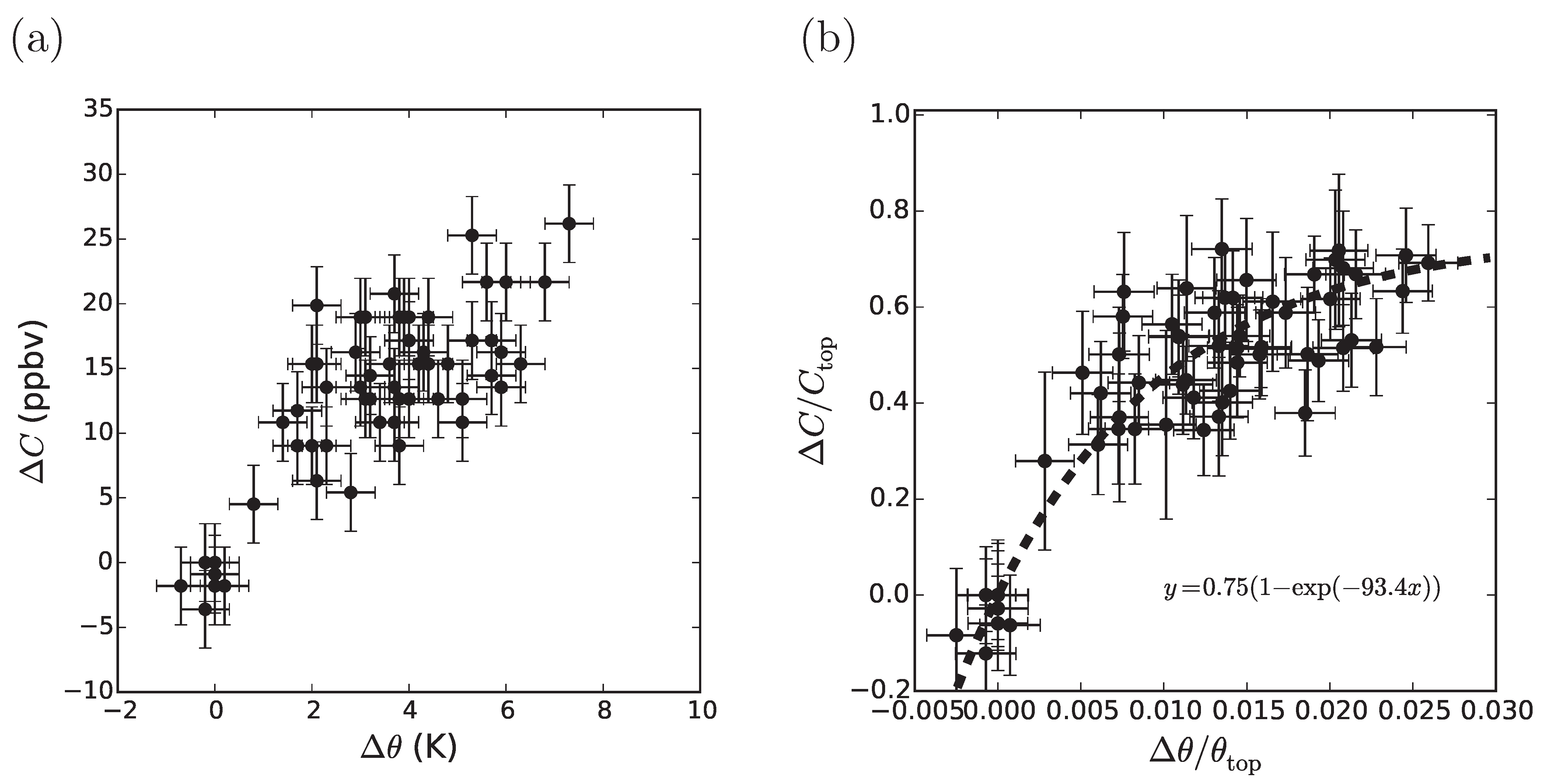
Figure 8a shows the relation between Δ θ and Δ C . Pearson’s correlation coefficient between Δ θ and Δ C was 0.83, which was found significant by Student’s t-test at the 1% significance level. This behavior agrees qualitatively with those obtained by previous authors [12,15].
In Figure 8b, the differences are normalized by the respective values at the top of Awajigatou. Assuming that Δ C = 0 when Δ θ = 0 and that Δ C / C top tends to a finite value of 0.75 (determined rather subjectively by visual inspection of Figure 8b), the following relation was obtained by the least-squares method,
Δ C C top = 0.75 1 exp - 93.4 Δ θ θ top
Pearson’s correlation coefficient between Δ θ / θ top and log 1 ( 1 / 0.75 ) Δ C / C top was 0.77, which was found significant by Student’s t-test at the 1% significance level.
Figure 8. Correlations between the temperature difference Δ θ and the ozone concentration difference Δ C at the bottom and top of Awajigatou in dimensional (a) and non-dimensional (b) forms. The dashed curve in panel (b) indicates Equation (4).
Atmosphere 06 00928 g008
This relation can be used to predict Δ C from Δ θ , which can be obtained at a much lower cost and effort than Δ C . The Equation (4) is specific to Awajigatou in winter, but similar relations at different sites in different seasons can be obtained by conducting similar measurements. Although not reported here in detail because of the small number of observation data, summer-time experiments resulted in considerably different coefficients in Equations (1) and (4).
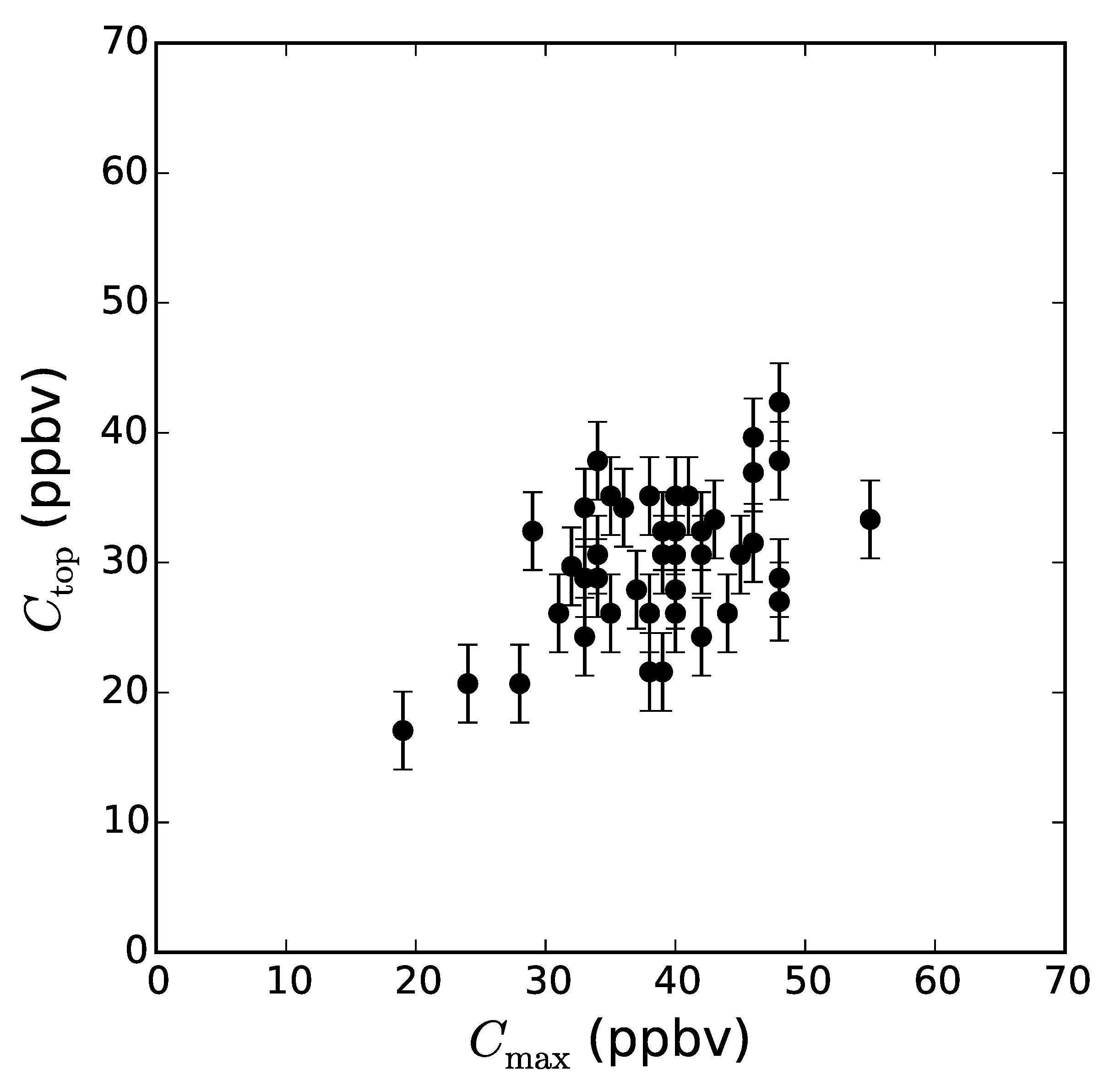
Under stable atmospheric conditions, C top , the value of C at the top of Awajigatou, represents the ozone concentration in the residual layer. As mentioned in Section 2.1, the pre-dawn residual layer contains ozone produced near the ground and brought up by convection during the previous day. The air mass in the residual layer may have been transported from outside the Dogo plain, but the surface-level ozone concentrations were generally well correlated in the surrounding regions. Therefore, C top is expected to be correlated with the daily maximum concentration C max of ozone on the previous day in the Dogo plain. Because the top of Awajigatou was not a location of occasional sudden signal drops, as shown in Figure 5, C top is a robust measure of ozone concentration at the summit elevation. It should be noted that this kind of data qualification was only possible by our spatially-continuous measurement. Figure 9 shows the scatter plot of C top and the daily maximum ozone concentration C max on the previous day at the Tomihisacho ambient air-monitoring station. Pearson’s correlation coefficient between C top and C max was 0.52, which was found significant by Student’s t-test at the 1% significance level. Generally, C max was larger than C top , consistent with no photochemical production, but continued mechanical and chemical destruction at night.
Figure 9. Correlation between the ozone concentration C top measured at the top of Awajigatou and the daily maximum ozone concentration C max observed at the Tomihisacho ambient air monitoring station on the previous day of the corresponding Awajigatou measurement.
Atmosphere 06 00928 g009

4. Conclusions

Vertical profiles of ozone concentration in the pre-dawn surface boundary layer were investigated by carrying a hand-held semiconductor-based ozone monitor while climbing up and down a relatively low mountain, Awajigatou, in Matsuyama, Japan. Under neutral atmospheric conditions, ozone concentration was approximately uniform from the foot to the top of Awajigatou, whereas under stable atmospheric conditions, ozone concentration became higher with elevation. The spatially-continuous data enabled robust determination of the concentrations at the bottom and top of Awajigatou. The vertical difference in the ozone concentration could be expressed as a function of the vertical difference in the potential temperature.
Although our current study was limited to a single path, mobile measurement by portable monitors can be extended to wider surveys in mountain areas. Such surveys will be useful not only in understanding the behavior of ozone in complex terrain, but also in determining optimal locations of long-term continuous monitoring stations at high elevation.

Acknowledgments

This work was supported by the “Joint Research Project on Formation Mechanism of Ozone, VOCs and PM2.5 and the Proposal of Countermeasure Scenarios” funded by the Japanese agencies JST (Japan Science and Technology Agency) and JICA (Japan International Cooperation Agency) under the SATREPS (Science and Technology Research Partnership for Sustainable Development) scheme.

Conflicts of Interest

The author declares no conflict of interest.

References

  1. Karnosky, D.F.; Skelly, J.M.; Percy, K.E.; Chappelka, A.H. Perspectives regarding 50 years of research on effects of tropospheric ozone air pollution on US forests. Environ. Pollut. 2007, 147, 489–506. [Google Scholar] [CrossRef] [PubMed]
  2. American Lung Association Fighting for Air. Available online: http://www.lung.org/healthy-air/outdoor/resources/ozone.html (accessed on 27 April 2015).
  3. Stocker, T.F.; Qin, D.; Plattner, G.-K.; Tignor, M.M.B.; Allen, S.K.; Boschung, J.; Nauels, A.; Xia, Y.; Bex, V.; Midgley, P.M. Intergovernmental Panel on Climate Change. Climate Change 2013 The Physical Science Basis; Cambridge University Press: Cambridge, UK, 2013; p. 1535. [Google Scholar]
  4. Vingarzan, R. A review of surface ozone background levels and trends. Atmos. Environ. 2004, 38, 3431–3442. [Google Scholar] [CrossRef]
  5. Aneja, V.P.; Claiborn, C.S.; Li, Z.; Murthy, A. Trends, seasonal variations, and analysis of high-elevation surface nitric acid, ozone, and hydrogen peroxide. Atmos. Environ. 1994, 28, 1781–1790. [Google Scholar] [CrossRef]
  6. Bytnerowicz, A.; Godzik, B.; Frączek, W.; Grodzińska, K.; Krywult, M.; Badea, O.; Barančok, P.; Blum, O.; Černy, M.; Godzik, S.; et al. Distribution of ozone and other air pollutants in forests of the Carpathian Mountains in central Europe. Environ. Pollut. 2002, 116, 3–25. [Google Scholar] [CrossRef]
  7. Gilge, S.; Plass-Duelmer, C.; Fricke, W.; Kaiser, A.; Ries, L.; Buchmann, B.; Steinbacher, M. Ozone, carbon monoxide and nitrogen oxides time series at four alpine GAW mountain stations in central Europe. Atmos. Chem. Phys. 2010, 10, 12295–12316. [Google Scholar] [CrossRef]
  8. Ou Yang, C.-F.; Lin, N.-H.; Sheu, G.-R.; Lee, C.-T.; Wang, J.-L. Seasonal and diurnal variations of ozone at a high-altitude mountain baseline station in East Asia. Atmos. Environ. 2012, 46, 279–288. [Google Scholar] [CrossRef]
  9. Sakata, M.; Suzuki, K.; Koshiji, T. Variations of wood delta C-13 for the past 50 years in declining Siebold’s beech (Fagus crenata) forests. Environ. Exp. Bot. 2001, 45, 33–41. [Google Scholar] [CrossRef]
  10. Brodin, M.; Helmig, D.; Oltmans, S. Seasonal ozone behavior along an elevation gradient in the Colorado Front Range Mountains. Atmos. Environ. 2010, 44, 5305–5315. [Google Scholar] [CrossRef]
  11. Cox, R.M. The use of passive sampling to monitor forest exposure to O3, NO2 and SO2: A review and some case studies. Environ. Pollut. 2003, 126, 301–311. [Google Scholar] [CrossRef]
  12. Aneja, V.P.; Arya, S.P.; Yongxian, L.; Murray, G.C.; Manuszak, T.L. Climatology of diurnal trends and vertical distribution of ozone in the atmospheric boundary layer in urban north Carolina. J. Air Waste Manag. Assoc. 2000, 50, 54–64. [Google Scholar] [CrossRef] [PubMed]
  13. Glaser, K.; Vogt, U.; Baumbach, G.; Volz-Thomas, A.; Geiss, H. Vertical profiles of O3, NO2, NOx, VOC, and meteorological parameters during the Berlin Ozone Experiment (BERLIOZ) campaign. J. Geophys. Res. 2003, 108, 8253. [Google Scholar] [CrossRef]
  14. Velasco, E.; Márquez, C.; Bueno, E.; Bernabé, R.M.; Sánchez, A.; Fentanes, O.; Wöhrnschimmel, H.; Cárdenas, B.; Kamilla, A.; Wakamatsu, S.; Molina, L.T. Vertical distribution of ozone and VOCs in the low boundary layer of Mexico City. Atmos. Chem. Phys. 2008, 8, 3061–3079. [Google Scholar] [CrossRef]
  15. Brodin, M.; Helmig, D.; Johnson, B.; Oltmans, S. Comparison of ozone concentrations on a surface elevation gradient with balloon-borne ozonesonde measurements. Atmos. Environ. 2011, 45, 5431–5439. [Google Scholar] [CrossRef]
  16. Williams, D.E.; Salmond, J.; Yung, Y.F.; Akaji, J.; Wright, B.; Wilson, J. Development of low-cost ozone and nitrogen dioxide measurement instruments suitable for use in an air quality monitoring network. In Proceedings of IEEE Sensors 2009 Conference, Christchurch, New Zealand, 25–28 October 2009; pp. 1099–1104.
  17. McKendry, I.G.; Lundgren, J. Tropospheric layering of ozone in regions of urbanized complex and/or coastal terrain: A review. Prog. Phys. Geogr. 2000, 24, 329–354. [Google Scholar] [CrossRef]
  18. Sillman, S. The relation between ozone, NOx and hydrocarbons in urban and polluted rural environments. Atmos. Environ. 1999, 33, 1821–1845. [Google Scholar] [CrossRef]
  19. McKendry, I.G.; Steyn, D.G.; Lundgren, J.; Hoff, R.M.; Strapp, W.; Anlauf, K.; Froude, F.; Martin, J.B.; Banta, R.M.; Olivier, L.D. Elevated ozone layers and vertical down-mixing over the Lower Fraser Valley, BC. Atmos. Environ. 1997, 31, 2135–2146. [Google Scholar] [CrossRef]
  20. Salmond, J.A.; McKendry, I.G. Secondary ozone maxima in a very stable nocturnal boundary layer: observations from the Lower Fraser Valley, BC. Atmos. Environ. 2002, 36, 5771–5782. [Google Scholar] [CrossRef]
  21. Lee, S.-M.; Fernando, H.J.S.; Princevac, M.; Zajic, D.; Sinesi, M.; McCulley, J.L.; Anderson, J. Transport and diffusion of ozone in the nocturnal and morning planetary boundary layer of the Phoenix valley. Environ. Fluid Mech. 2003, 3, 331–362. [Google Scholar] [CrossRef]
  22. Gundel, L.A.; Kirchstetter, T.W.; Spears, M.; Sullivan, D.P. Aircraft Cabin Environmental Quality Sensors; Lawrence Berkeley National Laboratory: Berkeley, CA, USA, 2010; p. LBNL–3382E. [Google Scholar]
  23. Naser, T.M.; Kanda, I.; Ohara, T.; Sakamoto, K.; Kobayashi, S.; Nitta, H.; Nataami, T. Analysis of traffic-related NOx and EC concentrations at various distances from major roads in Japan. Atmos. Environ. 2009, 43, 2379–2390. [Google Scholar] [CrossRef]

