1. Introduction
Clouds play a central role in the Arctic climate system. On the one hand, they reflect solar radiation cooling the Earth’s surface (cloud albedo effect), on the other hand, they absorb and (re-)emit terrestrial radiation warming the Earth’s surface (cloud greenhouse effect). Following Schneider [
1], cloud radiative forcing
![Atmosphere 03 00419 i005]()
is defined as difference between the net radiative fluxes under all-sky (
![Atmosphere 03 00419 i006]()
) and clear-sky (
![Atmosphere 03 00419 i007]()
) conditions.
![Atmosphere 03 00419 i006]()
is the sum of the net longwave (LW) and shortwave (SW) radiative fluxes, while
![Atmosphere 03 00419 i007]()
denotes those fluxes in a cloud-free but otherwise identical atmosphere.
While SW CRF depends on cloud transmittance, surface albedo, and the solar zenith angle, LW CRF is a function of cloud temperature, height, and emissivity as well as the background moisture (e.g., [
2,
3]). Furthermore, CRF varies depending on cloud phase, aerosol loading and whether convective or stratiform clouds are treated [
4,
5,
6]. The radiative effects of clouds and their impact on climate have been addressed in many observational and/or modeling studies. Although Ramanathan
et al. [
7] and Schneider [
1] have shown that clouds have a net cooling effect on the global climate, the studies of Walsh and Chapman [
8] and Intrieri
et al. [
9] have identified the net warming effect of clouds on the Arctic surface, except for a short period during summer when the cloud albedo effect outweighs the greenhouse effect.
Due to low surface temperatures, especially during polar night when there is no solar insolation, and advection of warmer air, ground-based or elevated temperature inversions occur frequently in the Arctic boundary layer (ABL) as demonstrated by Kahl
et al. [
10] and Zhang
et al. [
11]. Low Arctic temperatures are accompanied by comparably low absolute humidities. Apart from the presence of sufficient water vapor, airborne aerosol particles are prerequisites for cloud formation at normal supersaturations, acting either as cloud condensation nuclei or ice nuclei. Although Arctic air masses are normally cold, comparably dry and unpolluted [
12], high-latitudes are mainly characterized by the occurrence of so-called boundary layer clouds (BLCs, [
13,
14,
15]). These BLCs show large seasonal and interannual variability, which is reversely related to Arctic sea-ice variability [
16,
17].
A major problem in climate modeling is the subgrid-scale treatment of cloud processes, requiring sophisticated parameterizations that ideally include the whole complexity of cloud microphysics like water phase changes and precipitation processes. One of the most relevant obstacles is the sparse availability of cloud observations, especially in the inner Arctic (e.g., [
18]), impeding the formulation of sufficient cloud parameterizations and validation of model results. The deficient representation of model cloudiness [
19,
20,
21,
22] plays a relevant role in why the net CRF, or more specifically the cloud-radiation feedback [
3,
23,
24], is not definitely understood to date. Solomon
et al. [
25] have concluded that cloud feedbacks represent the largest source of uncertainty in climate sensitivity estimates. A particular shortcoming in modeling the Arctic climate is the limited representation of prevailing mixed-phase BLCs (e.g., [
26,
27,
28]). Climate models have also difficulties in accurately modeling the vertical structure of Arctic clouds associated with the presence of multiple cloud layers, a strong temperature inversion accompanied by rapid moisture decrease above cloud top, and vertical fluxes within the cloud that are decoupled from the surface fluxes [
26,
29]. All that complicates the determination of surface radiation fluxes, which are very sensitive to the modeled cloud microphysical characteristics. An intercomparison of Arctic regional climate models (RCMs) has confirmed the large uncertainty in simulated cloud cover [
30].
However, various Arctic-specific studies (e.g., [
31,
32]) have identified sources of error, e.g., that layered cloud formation requires a higher-order ABL parameterization. The cloud droplet radius has been found to impact surface LW CRF significantly by changing the emissivity of Arctic clouds [
33,
34], where the liquid component of mixed-phase clouds dominates radiative properties in general. For the liquid phase Morrison
et al. [
35] have found in part reasonable agreement between modeled and observed microphysical properties of Arctic mixed-phase clouds, while the ice microphysical properties have been identified as significantly biased. Morrison and Pinto [
27] have demonstrated that only two-moment bulk microphysical schemes enable the adequate simulation of ice nucleation and snow formation. On the one hand, Morrison
et al. [
36] have shown that these more sophisticated schemes can better reproduce the observed ratio of liquid and solid water in Arctic clouds; on the other hand, these schemes contain plenty of “tuning” parameters derived from lower-latitude measurements which might be inapplicable to Arctic climate conditions.
Convective and stratiform clouds differ considerably in their formation, characteristics (e.g., vertical wind speed, lifetime, horizontal/vertical extent), and generation of precipitation, arguing for individual parameterizations in climate models. Cumulus convection and associated dynamic cloud processes like organized or turbulent en-/detrainment are often modeled by so-called “mass flux schemes”. While several studies (e.g., [
37,
38]) have stated the minor importance of convective clouds in the Arctic, Pinto and Curry [
39], Curry
et al. [
40] and Rozwadowska and Cahalan [
41] have shown that even over Arctic sea ice shallow convective clouds emanate from open water in leads or polynyas. Further, Sato
et al. [
42] have recently identified that these cumuliform clouds rather become more important in the Arctic due to the shift from ice-covered to ice-free Arctic ocean during autumn which can be associated with more well-mixed than stable ABL structures. Convective cloud processes are even important for stratiform cloud formation, such that, e.g., convective detrainment at the cloud top can be a direct source for stratiform cloud cover. To simulate stratiform clouds, current climate models commonly use complex bulk microphysics (e.g., [
43,
44]) and apply either relative humidity cloud schemes (RH-Schemes) or statistical cloud schemes as pointed out by Tompkins [
45] or Zhu and Zuidema [
46].
The motivation to this study was to evaluate and possibly adapt the subgrid-scale parameterization of Arctic clouds in the single-column climate model (SCM) HIRHAM5-SCM. SCMs are considered as a useful tool for developing and evaluating physical parameterizations of climate models, and thus have been exploited in various Arctic studies [
47,
48,
49,
50]. Here, the newly designed SCM version of the most recent RCM version HIRHAM5 [
51] was exploited to analyze the two selectable cloud schemes for inner-Arctic climate conditions. The HIRHAM5-SCM setup and the applied cloud parameterizations are described in
Section 2. Results of the model evaluation are presented and discussed in
Section 3. In the first subsection, modeled height profiles of temperature and relative humidity as well as total cloud cover are validated against observations from NP-35 followed by some statistics. In the second subsection, some cloud-related model variables are discussed with respect to their credibility. An evaluation of simulated cloudiness, using either the RH-Scheme by Sundquist
et al. [
52] or the prognostic statistical cloud scheme (PS-Scheme) by Tompkins [
45], with two satellite-derived cloud data sets is shown afterwards. In
Section 4 several model parameters are analyzed by means of sensitivity experiments for their potential to adapt the cloud parameterization to Arctic climate conditions. Finally,
Section 5 contains conclusions and gives an outlook.
4. Parameter Sensitivity Studies
Sensitivity studies were conducted to assess the effect of modified model adjustment parameters (listed in
Table 1) on cloud-related variables relative to the reference run (see
Figure 3). One of the main goals was to identify suitable tuning parameters, which are potentially able to reduce the systematic overestimation of Arctic clouds in HIRHAM5-SCM. While the values of PS-Scheme tuning parameters are originally based on cloud resolving model simulations, tunable parameters of the cloud microphysics have been estimated by detailed microphysical models. These “tuning” parameters obviously need to be adapted for the usage in large-scale models as stated by Tompkins [
45] and Roeckner
et al. [
54]. Further adjustment of these parameters is likely required again when changing from the global to the regional scale, thus necessitating our sensitivity experiments.
Each sensitivity experiment comprised a simulation over 13 months by analogy to the reference run but using a modified value of a single model parameter. Although every tuning parameter was varied within a certain parameter range (see
Table 1), the following discussions will basically be restricted to one lower and higher value, respectively, since the main conclusions remain unchanged. Based on the simulations, differences between respective sensitivity run (hereinafter “SENS”) and reference run (hereinafter “CTRL”) were computed, and zero-cases were neglected. To quantify the impact of a certain parameter change, relative frequencies of “positive differences” (
![Atmosphere 03 00419 i093]()
) were calculated for several cloud-related model variables both with respect to all 13 simulated months and the periods with moderate (WP) and high (SP)
![Atmosphere 03 00419 i027]()
in the reference run. Let
![Atmosphere 03 00419 i094]()
be the relative frequency of positive differences, then the percental decrease (
![Atmosphere 03 00419 i095]()
) or increase (
![Atmosphere 03 00419 i096]()
) of a certain model variable relative to the reference run can be computed using the formula
![Atmosphere 03 00419 i097]()
. The results are listed in
Table 4 and
Table 5 either with respect to
lower or
higher tuning parameters.
Table 4.
Percental decrease/increase of several model variables due to
lower parameter values (
![Atmosphere 03 00419 i098]()
,
![Atmosphere 03 00419 i099]()
,
![Atmosphere 03 00419 i100]()
,
![Atmosphere 03 00419 i157]()
,
![Atmosphere 03 00419 i158]()
,
![Atmosphere 03 00419 i101]()
,
![Atmosphere 03 00419 i102]()
,
![Atmosphere 03 00419 i103]()
) relative to the default (
Table 1) for the entire 13-month-long simulations (“all”) as well as the winter (WP) and summer (SP) periods as introduced in
Section 3.2.1.
Table 5.
Same as
Table 4 but for
higher parameter values (
![Atmosphere 03 00419 i112]()
,
![Atmosphere 03 00419 i113]()
,
![Atmosphere 03 00419 i114]()
,
![Atmosphere 03 00419 i115]()
,
![Atmosphere 03 00419 i159]()
,
![Atmosphere 03 00419 i160]()
,
![Atmosphere 03 00419 i161]()
,
![Atmosphere 03 00419 i116]()
).
4.1. Modified Adjustment Parameters of PS-Scheme
As introduced by
Section 2.2 the PS-Scheme includes the two adjustment parameters
![Atmosphere 03 00419 i028]()
and
K. The former was varied in the co-domain
![Atmosphere 03 00419 i117]()
, following the restrictions
![Atmosphere 03 00419 i118]()
and
![Atmosphere 03 00419 i119]()
for the beta distribution shape parameters to obtain only unimodal distributions. Also according to Tompkins [
45], the conditions
![Atmosphere 03 00419 i120]()
and
![Atmosphere 03 00419 i121]()
were retained to exclude distributions with negative skewness.
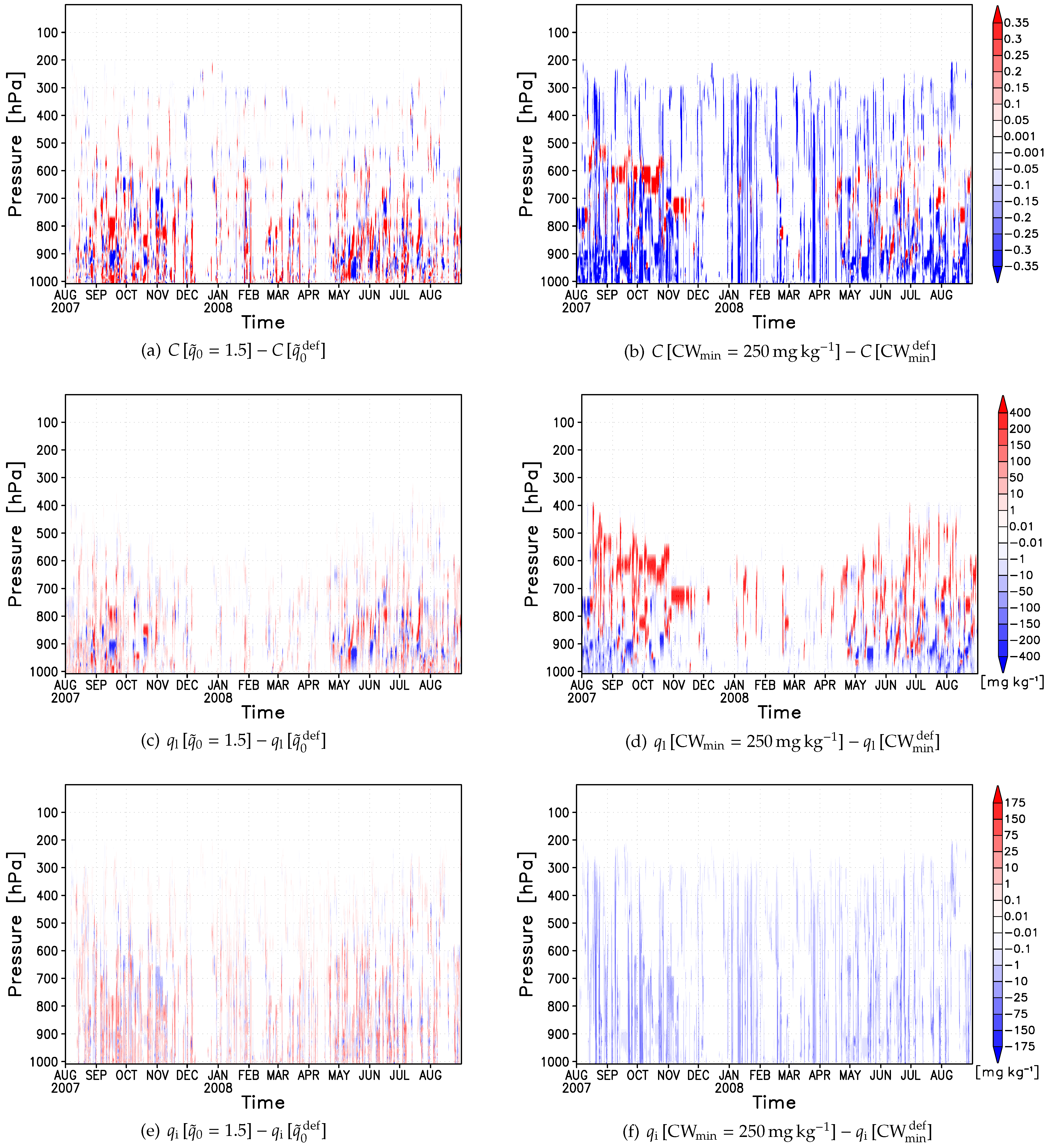
Figure 5.
Difference plots (SENS minus CTRL) of simulated fractional cloud cover (
top), cloud water content (
middle), and cloud ice content (
bottom) for one lower value of the PS-Scheme adjustment parameter
![Atmosphere 03 00419 i001]()
(
left column) and one higher value of the tunable parameter
![Atmosphere 03 00419 i002]()
(
right column), with
![Atmosphere 03 00419 i123]()
and
![Atmosphere 03 00419 i124]()
. These sensitivity experiments were conducted at the NP-35 start position simulating from 1 August 2007 to 31 August 2008 by analogy to the reference run (
Figure 3).
The third column of
Table 4 and
Table 5 reveal that overall a lower (higher) value of
![Atmosphere 03 00419 i028]()
leads to a reduction of (rise in)
![Atmosphere 03 00419 i027]()
. Indeed mid- and high-level clouds decrease significantly due to lower parameter values while low-level clouds tend to slightly increase (see
Figure 5(a)). One possible reason for the increase at lower levels might be very low saturation water contents due to cold temperatures in the relatively wet boundary layer over the Arctic Ocean favoring cloud formation. Although lower values of
![Atmosphere 03 00419 i028]()
are able to reduce
![Atmosphere 03 00419 i027]()
and rise
![Atmosphere 03 00419 i080]()
(overall increase in
![Atmosphere 03 00419 i009]()
suggested by
Figure 5(c)) as well as
![Atmosphere 03 00419 i084]()
, the overestimation of
![Atmosphere 03 00419 i086]()
is strengthened (overall increase in
![Atmosphere 03 00419 i008]()
suggested by
Figure 5(e)). Both
![Atmosphere 03 00419 i082]()
and
![Atmosphere 03 00419 i083]()
rise amplifying the overestimation of
![Atmosphere 03 00419 i087]()
as well.
The second adjustment parameter
K, which relates the increase in the skewness parameter
![Atmosphere 03 00419 i024]()
to the detrainment of cloud condensate, was varied in the co-domain
![Atmosphere 03 00419 i125]()
. However, modifying this parameter only leads to temporary local changes of
C (not shown), and overall
![Atmosphere 03 00419 i027]()
remains almost unaffected. This can be attributed to the minor role of convection in cloud formation over the ice-covered Arctic Ocean, unless open water areas in terms of polynyas or leads coexist. Other cloud-related model variables either remain almost unchanged or increase in part significantly by changes in
K. Both the overestimation of
![Atmosphere 03 00419 i008]()
(
![Atmosphere 03 00419 i086]()
) and
![Atmosphere 03 00419 i087]()
is strengthened. Furthermore, only higher parameter values of
K enable convective precipitation during wintertime (WP) explaining the increase of 100% in the fourth column of
Table 5.
4.2. Modified Tuning Parameters of Cloud Microphysics
The following discussions will basically concentrate on tuning parameters of the cloud microphysics, which can reduce
![Atmosphere 03 00419 i027]()
based on
Table 4 and
Table 5, and conclusions are summarized in
Table 6.
Table 6.
Overall effect on cloud-related model variables due to modification of a single model tuning parameter enabling the reduction of
![Atmosphere 03 00419 i065]()
relative to the default parameter value (see
Table 1 and
Figure 4). Effects that potentially improve model results are marked by a ‘+’, negative influences are indicated by a ‘−’.
Table 6.
Overall effect on cloud-related model variables due to modification of a single model tuning parameter enabling the reduction of ![Atmosphere 03 00419 i065]() relative to the default parameter value (see Table 1 and Figure 4). Effects that potentially improve model results are marked by a ‘+’, negative influences are indicated by a ‘−’.
relative to the default parameter value (see Table 1 and Figure 4). Effects that potentially improve model results are marked by a ‘+’, negative influences are indicated by a ‘−’.
| Parameter | Changes due to lower parameter value | Changes due to higher parameter value |
|---|
![Atmosphere 03 00419 i047]() | 1.5 | 20 |
| | ![Atmosphere 03 00419 i127]() reduction of reduction of ![Atmosphere 03 00419 i128]() and and ![Atmosphere 03 00419 i111]() | ![Atmosphere 03 00419 i127]() rise in rise in ![Atmosphere 03 00419 i129]() ( ( ![Atmosphere 03 00419 i130]() ) but reduction of ) but reduction of ![Atmosphere 03 00419 i131]() ( ( ![Atmosphere 03 00419 i132]() ); ); |
| | ![Atmosphere 03 00419 i127]() rise in rise in ![Atmosphere 03 00419 i129]() ( ( ![Atmosphere 03 00419 i130]() ) ) | effect is small (large) for ![Atmosphere 03 00419 i131]() ( ( ![Atmosphere 03 00419 i129]() ) ) |
| | ![Atmosphere 03 00419 i133]() rise in rise in ![Atmosphere 03 00419 i131]() ( ( ![Atmosphere 03 00419 i132]() ) ) | ![Atmosphere 03 00419 i133]() rise in rise in ![Atmosphere 03 00419 i128]() , , ![Atmosphere 03 00419 i111]() , , ![Atmosphere 03 00419 i134]() , and , and ![Atmosphere 03 00419 i135]() |
| | ![Atmosphere 03 00419 i133]() rise in rise in ![Atmosphere 03 00419 i134]() and and ![Atmosphere 03 00419 i135]() | |
![Atmosphere 03 00419 i050]() | ![Atmosphere 03 00419 i136]() | ![Atmosphere 03 00419 i137]() |
| | ![Atmosphere 03 00419 i127]() rise in rise in ![Atmosphere 03 00419 i129]() ( ( ![Atmosphere 03 00419 i130]() ) but reduction of ) but reduction of ![Atmosphere 03 00419 i131]() ( ( ![Atmosphere 03 00419 i132]() ); ); | ![Atmosphere 03 00419 i127]() significant reduction of significant reduction of ![Atmosphere 03 00419 i128]() , , ![Atmosphere 03 00419 i111]() |
| | effect is more pronounced than for higher | ![Atmosphere 03 00419 i127]() reduction of reduction of ![Atmosphere 03 00419 i135]() |
| | ![Atmosphere 03 00419 i047]() and more significant for and more significant for ![Atmosphere 03 00419 i129]() | ![Atmosphere 03 00419 i133]() reduction of reduction of ![Atmosphere 03 00419 i129]() ( ( ![Atmosphere 03 00419 i130]() ) but rise in ) but rise in ![Atmosphere 03 00419 i131]() ( ( ![Atmosphere 03 00419 i132]() ) ) |
| | ![Atmosphere 03 00419 i133]() rise in rise in ![Atmosphere 03 00419 i128]() , , ![Atmosphere 03 00419 i111]() , , ![Atmosphere 03 00419 i134]() , and , and ![Atmosphere 03 00419 i135]() | and ![Atmosphere 03 00419 i134]() |
![Atmosphere 03 00419 i053]() | 5 | 100 |
| | ![Atmosphere 03 00419 i127]() ![Atmosphere 03 00419 i129]() ( ( ![Atmosphere 03 00419 i130]() ) rises but reduction of ) rises but reduction of ![Atmosphere 03 00419 i135]() | ![Atmosphere 03 00419 i127]() rise in rise in ![Atmosphere 03 00419 i129]() ( ( ![Atmosphere 03 00419 i130]() ) but reduction of ) but reduction of ![Atmosphere 03 00419 i131]() ( ( ![Atmosphere 03 00419 i132]() ); ); |
| | ![Atmosphere 03 00419 i133]() rise in all other regarded model variables rise in all other regarded model variables | effect is large (small) for ![Atmosphere 03 00419 i131]() ( ( ![Atmosphere 03 00419 i129]() ) ) |
| | | ![Atmosphere 03 00419 i127]() significant decrease in significant decrease in ![Atmosphere 03 00419 i128]() , , ![Atmosphere 03 00419 i111]() |
| | | ![Atmosphere 03 00419 i133]() rise in rise in ![Atmosphere 03 00419 i134]() and and ![Atmosphere 03 00419 i135]() |
![Atmosphere 03 00419 i061]() | ![Atmosphere 03 00419 i138]() | ![Atmosphere 03 00419 i139]() |
| | ![Atmosphere 03 00419 i127]() rise in rise in ![Atmosphere 03 00419 i129]() ( ( ![Atmosphere 03 00419 i130]() ) but reduction of ) but reduction of ![Atmosphere 03 00419 i131]() ( ( ![Atmosphere 03 00419 i132]() ), ), | ![Atmosphere 03 00419 i127]() ![Atmosphere 03 00419 i129]() ( ( ![Atmosphere 03 00419 i130]() ) rises ) rises |
| | where effect is significant for ![Atmosphere 03 00419 i131]() and and ![Atmosphere 03 00419 i129]() | ![Atmosphere 03 00419 i133]() rise in all remaining model variables rise in all remaining model variables |
| | ![Atmosphere 03 00419 i127]() reduction of reduction of ![Atmosphere 03 00419 i128]() , , ![Atmosphere 03 00419 i111]() | |
| | ![Atmosphere 03 00419 i133]() increase in increase in ![Atmosphere 03 00419 i134]() and and ![Atmosphere 03 00419 i135]() | |
To assess the impact of modified
![Atmosphere 03 00419 i042]()
, sensitivity experiments were conducted in the wide range between zero and
![Atmosphere 03 00419 i140]()
. Note that
![Atmosphere 03 00419 i042]()
impacts model results by ensuring nonzero
![Atmosphere 03 00419 i008]()
and
![Atmosphere 03 00419 i009]()
regardless of the applied cloud scheme (see
Table 1). As a working hypothesis, lower (higher)
![Atmosphere 03 00419 i042]()
should result in rising (declining) cloud cover. This is generally confirmed by the fifth column of
Table 4 and
Table 5. Higher
![Atmosphere 03 00419 i042]()
lead to significant decrease in
![Atmosphere 03 00419 i027]()
, and very high parameter values are even able to prevent the formation of clouds. While low- and high-level clouds tend to decline monotonically, mid-level clouds first seem to increase but finally decrease as well (suggested by
Figure 5(b)). Despite the ability to reduce the overestimation of
![Atmosphere 03 00419 i027]()
, higher
![Atmosphere 03 00419 i042]()
amplify the over- and underestimation of
![Atmosphere 03 00419 i086]()
and
![Atmosphere 03 00419 i080]()
, respectively. During the entire simulation period
![Atmosphere 03 00419 i008]()
decreases below 900h but significantly increases above 900h, while
![Atmosphere 03 00419 i009]()
decreases monotonically (see
Figure 5(d,f)). Furthermore, higher
![Atmosphere 03 00419 i042]()
amplify the overestimation of
![Atmosphere 03 00419 i082]()
while
![Atmosphere 03 00419 i083]()
and
![Atmosphere 03 00419 i084]()
drop.
The autoconversion rate
![Atmosphere 03 00419 i141]()
, which controls the conversion from (supercooled) cloud droplets to rain drops and thus the cloud lifetime effect, was found to be the next promising tuning parameter. This parameter was varied in the co-domain
![Atmosphere 03 00419 i142]()
.
Figure 6(a) and the sixth column of
Table 4 and
Table 5 confirm that only higher parameter values might be able to improve simulated cloudiness. Here, the increase in
![Atmosphere 03 00419 i027]()
during wintertime (WP) is outweighed by the decrease during summertime (SP). Furthermore, higher
![Atmosphere 03 00419 i141]()
are able to reduce the over- and underestimation of
![Atmosphere 03 00419 i086]()
and
![Atmosphere 03 00419 i080]()
, respectively. For
![Atmosphere 03 00419 i008]()
and
![Atmosphere 03 00419 i009]()
this effect is more difficult to identify from
Figure 6(c,e) due to temporary local changes. As expected,
![Atmosphere 03 00419 i082]()
and
![Atmosphere 03 00419 i083]()
rise in case of higher
![Atmosphere 03 00419 i141]()
amplifying the overestimation of
![Atmosphere 03 00419 i087]()
, while
![Atmosphere 03 00419 i084]()
is more or less unaffected.
Finally, the cloud ice threshold
![Atmosphere 03 00419 i143]()
was identified as promising tuning parameter. This parameter controls the Bergeron–Findeisen process, which explains the growth of ice crystals at the expense of cloud droplets in mixed-phase clouds due to lower vapor pressures over ice than over water at subfreezing temperatures. Lohman
et al. [
66] have pointed out that as soon as the threshold of cloud ice content is exceeded a supercooled water cloud will glaciate immediately in the model. In the standard ECHAM5 code the remaining cloud water is not evaporated to deposit onto existing ice crystals but remaining cloud droplets have to either freeze or grow to precipitable sizes in subsequent time steps. For the sake of completeness
![Atmosphere 03 00419 i143]()
was varied from zero to
![Atmosphere 03 00419 i144]()
. As shown by
Figure 6(b) and the last column of
Table 4 and
Table 5, lower
![Atmosphere 03 00419 i143]()
are also able to reduce the overestimation of simulated Arctic clouds. Furthermore, a lower parameter value is most suitable to improve the modeled ratio of
![Atmosphere 03 00419 i008]()
to
![Atmosphere 03 00419 i009]()
(overall reduction of
![Atmosphere 03 00419 i008]()
but rise in
![Atmosphere 03 00419 i009]()
, see
Figure 6(d,f)), which can be associated with the most significant reduction of
![Atmosphere 03 00419 i086]()
but rise in
![Atmosphere 03 00419 i080]()
. While
![Atmosphere 03 00419 i027]()
decreases and
![Atmosphere 03 00419 i087]()
remains almost unchanged,
![Atmosphere 03 00419 i084]()
increases overall.
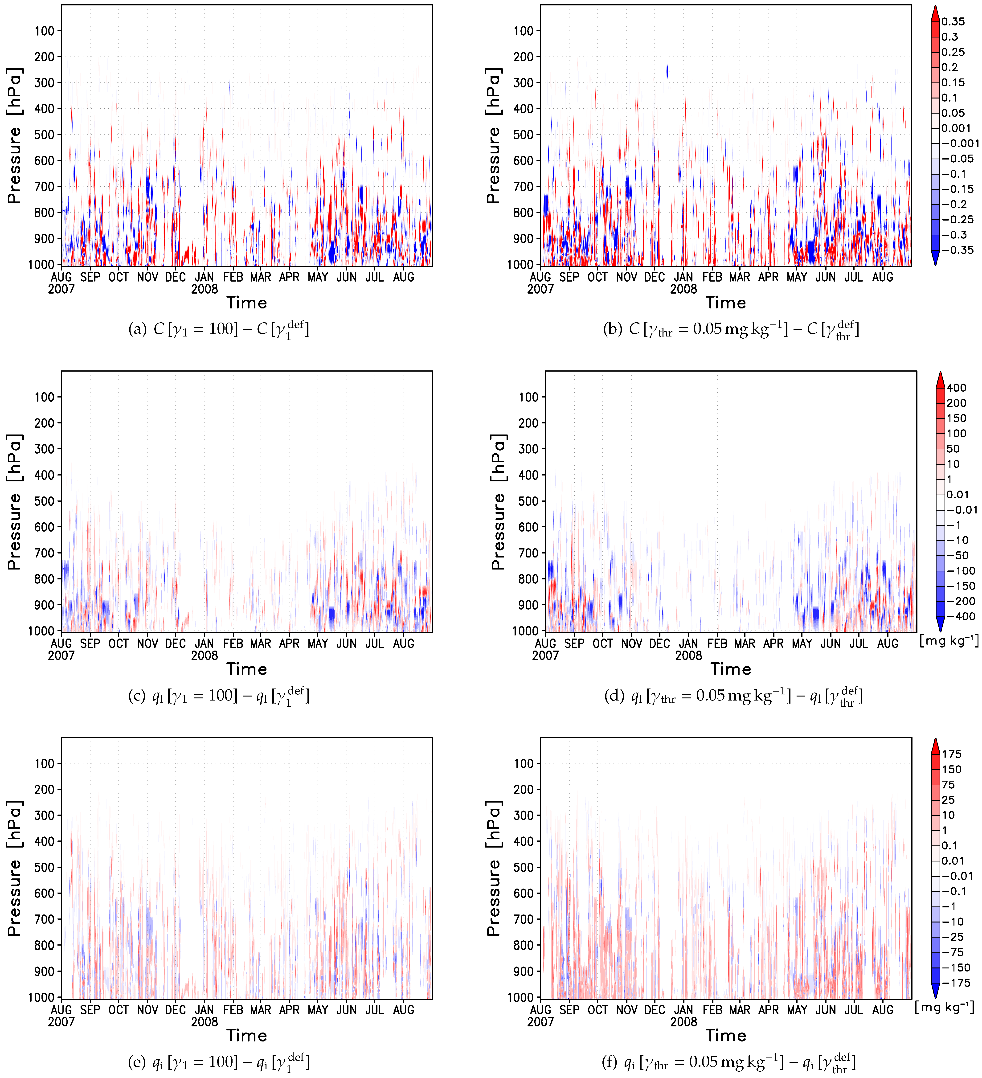
Figure 6.
Difference plots (SENS minus CTRL) of simulated fractional cloud cover (
top), cloud water content (
middle), and cloud ice content (
bottom) for one higher value of the tunable parameter
![Atmosphere 03 00419 i003]()
(
left column) and one lower value of the tunable parameter
![Atmosphere 03 00419 i110]()
(
right column), with
![Atmosphere 03 00419 i146]()
and
![Atmosphere 03 00419 i147]()
. These sensitivity experiments were conducted at the NP-35 start position simulating from 1 August 2007 to 31 August 2008 by analogy to the reference run (
Figure 3).
Figure 7 shows the comparison of monthly averaged
![Atmosphere 03 00419 i027]()
by analogy to
Section 3.2.2. Here, only the annual cycles of the best-fit parameters (
green curves), based on the best combination of lowest 13-month-mean of
![Atmosphere 03 00419 i027]()
and overall RMSE, are shown in addition to the annual cycle produced by MODIS (
black curve) and using the default values (
blue curve), respectively. Note that MODIS and the HIRHAM5-SCM reference run (using the PS-Scheme) produced averaged
![Atmosphere 03 00419 i027]()
of 64.8% and 78.2%, respectively with an overall RMSE of 18.4% (see
Table 3). Thus,
Figure 7 confirms that higher
![Atmosphere 03 00419 i042]()
(averaged
![Atmosphere 03 00419 i027]()
of 77.3% and overall RMSE of 17.2% for
![Atmosphere 03 00419 i149]()
) and
![Atmosphere 03 00419 i141]()
(averaged
![Atmosphere 03 00419 i027]()
of 77.8% and overall RMSE of 17.3% for
![Atmosphere 03 00419 i150]()
) as well as lower
![Atmosphere 03 00419 i028]()
(averaged
![Atmosphere 03 00419 i027]()
of 76.5% and overall RMSE of 17.9% for
![Atmosphere 03 00419 i151]()
) and
![Atmosphere 03 00419 i143]()
(averaged
![Atmosphere 03 00419 i027]()
of 74.9% and overall RMSE of 14.1% for
![Atmosphere 03 00419 i152]()
) reduce simulated Arctic cloud cover, where the latter might be the most promising tuning parameter to improve cloud-related variables in the model.
Figure 7.
Monthly means of
![Atmosphere 03 00419 i065]()
(in %) from August 2007 to August 2008 referring to the NP-35 start position. The results originate from MODIS (
black line) satellite observations, and HIRHAM5-SCM simulations using either the PS-Scheme and default model parameters (
blue line) or the PS-Scheme with a single modified tuning parameter (
green lines).
Figure 7 also reveals that all four tuning parameters are able to reduce
![Atmosphere 03 00419 i027]()
during May 2008 while only modified
![Atmosphere 03 00419 i028]()
and
![Atmosphere 03 00419 i143]()
improve the simulation of Arctic clouds during October 2007. In the former case, the enhanced cloud formation due to unrealistic turbulent moisture fluxes could be either partially compensated due to more efficient precipitation processes (for
![Atmosphere 03 00419 i141]()
and
![Atmosphere 03 00419 i143]()
) or through the partial suppression of cloud formation (for
![Atmosphere 03 00419 i028]()
and
![Atmosphere 03 00419 i042]()
). In the latter case, both the more deficient simulation of the ABL structure and the overestimated cloud top radiative cooling could not be significantly improved by changing tuning parameters of the cloud microphysics, except for
![Atmosphere 03 00419 i143]()
. The most significant impact through reduced
![Atmosphere 03 00419 i143]()
in both cases can be explained with the more efficient Bergeron–Findeisen process which results in faster growing cloud ice particles and finally enhanced snow fall.
5. Conclusions
A SCM version of the atmospheric RCM HIRHAM5 was developed to analyze the representation of Arctic clouds. HIRHAM5-SCM was exploited as test bed for evaluating the cloud cover schemes of the ECHAM5 parameterization package, the RH-Scheme by Sundquist
et al. [
52] and the more sophisticated PS-Scheme by Tompkins [
45].
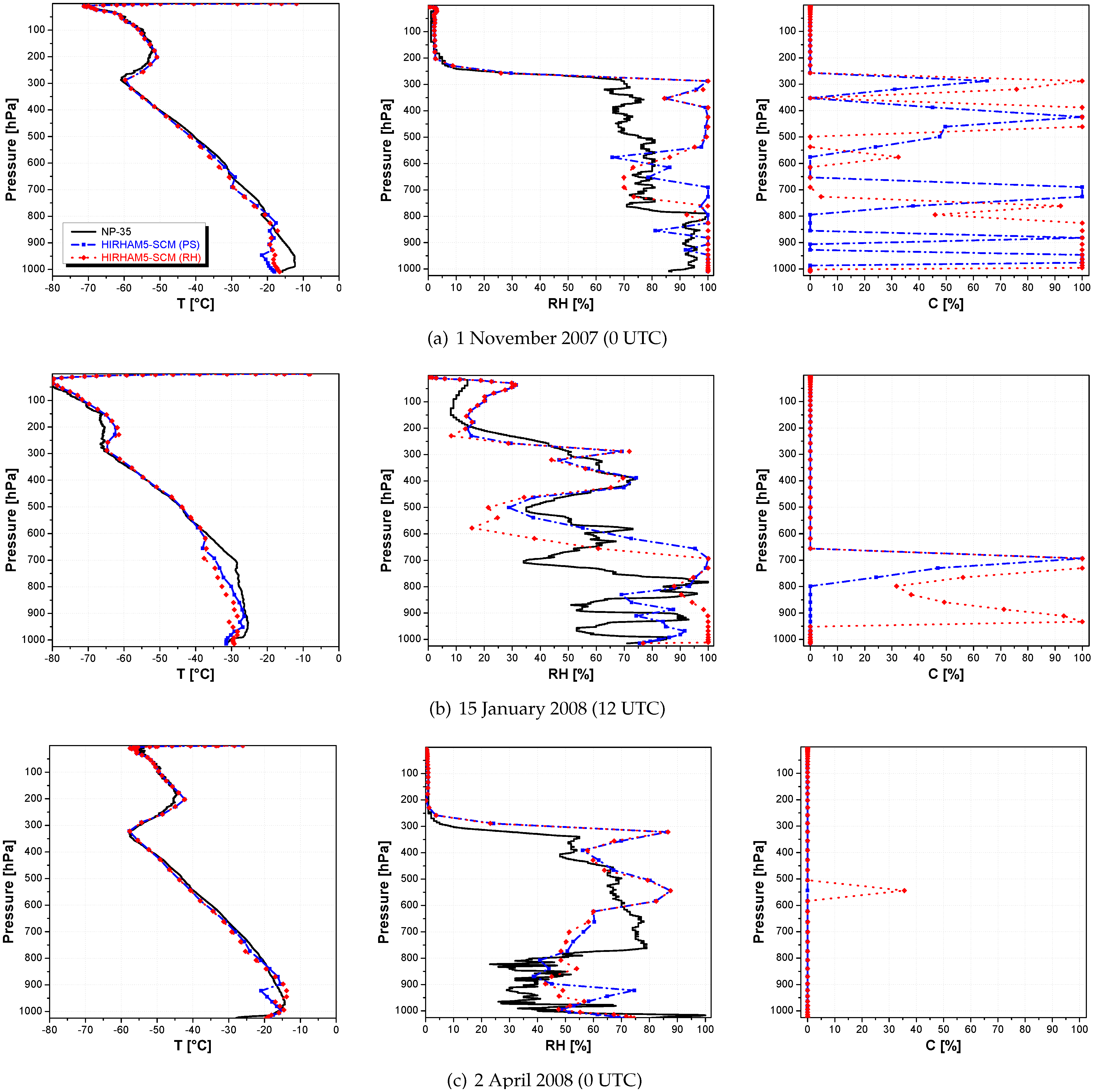
Observations from the 35th Russian North Pole drifting station (NP-35) were used to validate the model. Above the Arctic boundary layer (ABL), simulated and observed temperature profiles agree fairly well. In contrast, the more pronounced vertical variability of relative humidity is inadequately reproduced. Primarily the RH-Scheme produces clouds at incorrect altitudes. The PS-Scheme enables to better simulate the observed correlation between the occurrence of boundary layer clouds (BLCs) and capping strong temperature inversion as well as rapid moisture decrease. Further, the PS-Scheme results in higher correlations between the simulated and the measured temperature and humidity profiles. Nevertheless, the model has difficulties in simulating the ABL, most likely due to unrealistic turbulent exchange under extremely stable conditions.
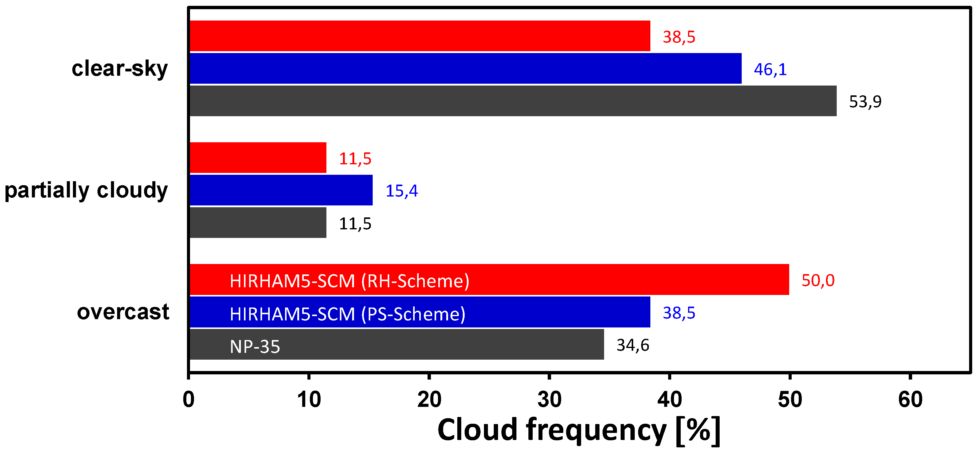
The evaluation of relative frequencies of simulated clear-sky, partially cloudy, and (totally) overcast cases revealed underestimation of clear-sky and overestimation of overcast conditions as compared to ground-based observations at NP-35. Both biases are significantly larger when using the RH-Scheme, even though the frequency of partially cloudy conditions agrees well. Overall, the overestimation of cloudy cases (sum of partially cloudy and overcast cases) is reduced by the PS-Scheme.
Independent from the used cloud scheme, the higher frequency of occurrence of modeled low-level clouds during summer (JJA) and autumn (SON) is in accordance with the frequently observed presence of summertime BLCs [
13,
14]. However, the PS-Scheme simulates cloud formation and dissipation more realistically, since the cloud cover is directly linked to sources and sinks (like turbulence, convection, and microphysics), enabling the simulation of frequently observed abrupt changes between overcast and clear-sky conditions.
The validation of the simulated annual cycle of total cloud cover against ISCCP-D2 and MODIS satellite observations showed qualitative agreement with MODIS in terms of higher cloud cover in summer and lower cloud cover in winter. The annual cycle of ISCCP-D2 is reversed and might be unrealistic as has already been pointed out by Schweiger
et al. [
71] and as is suggested by comparison with the ground-based observations at NP-35.
The qualitative agreement with MODIS is independent from the cloud cover scheme, but the RH-Scheme systematically overestimates the cloud cover, while the PS-Scheme shows reduced biases and pretty good agreement from November to January. However, the transition from high cloud cover in summer to lower cloud cover in winter and vice versa is shifted to the cold season in either case, accompanied by large biases in October and May.
All in all, the PS-Scheme enables an improved simulation of Arctic clouds as compared to the RH-Scheme, but it still shows a systematic overestimation of Arctic cloud cover. Several tunable parameters were analyzed by means of sensitivity studies to identify parameters which potentially enable the adaptation of the cloud parameterization to Arctic climate conditions. The resulting recommendations are summarized below:
• Lower values of
![Atmosphere 03 00419 i047]()
, the parameter that determines the shape of the symmetric beta distribution in the PS-Scheme, result in a reduction of total cloud cover (
![Atmosphere 03 00419 i153]()
best fit to MODIS), decreased underestimation of cloud ice, but increased overestimation of cloud water and precipitation.
• Higher values of the minimum cloud water content
![Atmosphere 03 00419 i050]()
result in a reduction of clouds (even up to their total disappearance) and consequently decreased overestimation of total cloud cover (
![Atmosphere 03 00419 i154]()
best fit to MODIS), but also in increased overestimation/underestimation of cloud water/cloud ice and increased overestimation of precipitation. Instead of applying the same value of
![Atmosphere 03 00419 i050]()
to cloud water and cloud ice, it is suggested using different thresholds, since cloud water contents are typically about one magnitude higher than cloud ice contents in Arctic clouds (e.g., [
28,
47]).
• Higher values of the autoconversion rate
![Atmosphere 03 00419 i053]()
, which controls the local rain production and thus the cloud lifetime, result in decreased overestimation of total cloud cover (
![Atmosphere 03 00419 i155]()
best fit to MODIS), decreased overestimation/underestimation of cloud water/cloud ice, but increased overestimation of precipitation as was expected.
• Lower values of the cloud ice threshold
![Atmosphere 03 00419 i061]()
, which controls the efficiency of the Bergeron–Findeisen process, turned out to be most suitable for reducing the overestimation of total cloud cover (
![Atmosphere 03 00419 i156]()
best fit to MODIS) and result additionally in decreased overestimation/underestimation of cloud water/cloud ice, but also increased overestimation of precipitation.
The best-fit parameters suggested by this study need to be examined for their performance in the three-dimensional model version HIRHAM5. Liu
et al. [
77] have identified the possible underestimation of MODIS relative to CloudSat-CALIPSO cloud amount especially over the ice-covered Arctic ocean. It is therefore planned to validate cloud-related variables simulated by HIRHAM5 against observations from the Multiangle Imaging SpectroRadiometer (MISR) and Cloud Aerosol Lidar with Orthogonal Polarization (CALIOP). Since changes in modeled cloud fraction and total precipitation are anti-correlated, extensive validation against precipitation observations is required. This is currently ongoing work.

 is defined as difference between the net radiative fluxes under all-sky (
  ) and clear-sky (
  ) conditions.
  , cloud ice content
  , and surface pressure
  . The total tendency of a prognostic variable can be split into a physical (diabatic) and a dynamical (adiabatic) part, where the former describes temporal changes due to subgrid-scale processes like radiation, cloud formation, and vertical diffusion. HIRHAM5-SCM calculates physical tendencies explicitly, using an explicit Euler forward time stepping scheme with 10 min time step. Since the dynamical part cannot be computed by a SCM, HIRHAM5-SCM uses prescribed
 represents the grid box mean and
  the critical threshold of relative humidity. The latter decreases exponentially from 90% near the surface to 70% at higher altitudes (see [43]) and controls the onset of cloud formation.
 is explicitly specified by a probability density function (PDF) in terms of the beta distribution
  . Note that
  defines the cloud condensate as sum of cloud water and cloud ice content. The scheme includes prognostic equations for the higher order moments of the beta distribution, namely variance (distribution width) and skewness, which are linked to subgrid-scale processes like turbulence, convection, and microphysics (see [45]). Fractional cloud cover is then computed as integral over the supersaturation part (
  ) of the actual beta distribution:
 denotes the saturation water content.
  defines the ratio of incomplete to complete beta function, where
  with the lower distribution bound
  , and
, and  and
and  are the shape parameters of the beta distribution. Following Tompkins [45], the shape parameter
  ). In contrast,
 is calculated by the model using a maximum-random overlap assumption with respect to computed values of C in the respective model levels. Clouds in contiguous layers are maximally overlapped, while clouds separated by one or more clear-sky layers are randomly overlapped.
 and K. The first parameter
 and
and  denote the vertical and horizontal mixing time scales (see [45]). While
  depends on the mixing length and the turbulent kinetic energy,
  is neglected since horizontal mixing is not available in the SCM version. Turbulent mixing processes due to subgrid-scale eddies mainly lead to a reduction of skewness and, therefore, to an aspiration towards a symmetric beta distribution. Currently,
  is used as default value, restricting the skewness of
  .
. , appears in the convection term of the skewness equation
 is the mean air density and
 represents the mass flux of cloud condensate due to convective updraft, where
  . The superscript “cu” denotes that the respective variables are calculated by the cumulus convection scheme, which is based on the mass flux scheme of Tiedtke [63] with modifications for penetrative convection according to Nordeng [64].
 , which avoids negative
  and
and  , C will be set to zero. Thus, clouds will only appear in the PS-Scheme if at least one of the two variables exceeds
  was used in accordance to Zhang and Lohmann [49].
 , which is not mentioned by Roeckner et al. [54], the notation conforms to the ECHAM5 documentation.


 using either the PS-Schem or RH-Scheme. In the notation “yyyy-mm-dd_hh”, “yyyy” = year, “mm” = month, “dd” = day and “hh” = hour. Dates in bold type are discussed in detail in Section 3.1.1.

 was computed in every model level with respect to NP-35 measurements. Since none of the studied NP-35 radiosondes rose higher than 7h and at least two radiosonde measurements should be available for a certain pressure height,
  ) were calculated within the entire atmospheric column independently from the applied cloud scheme. While the temperature correlation was consistently very high (
  ) above the 30th model level (about 200h), the strength of the linear relation decreased below and became minimal in the ABL. This was confirmed by vertically averaged correlation coefficients
  computed either for the entire SCM-column or the 10 model levels closest to the surface. While the PS-Scheme produced
  (13 to 60 model level) and
  (51 to 60 model level), the RH-Scheme showed slightly lower mean correlations of 0.94 and 0.85, respectively. HIRHAM5-SCM generally produced comparably low temperature correlations in the three model levels closest to the surface (
  for RH-Scheme) indicating incorrect turbulent heat fluxes. Interestingly, lowest values of
  (up to 0.76) appeared around the 52nd model level (about 930h), which might be explained with an incorrect coupling between ABL and the free troposphere in the model. The RH-Scheme produced slightly higher correlation coefficients between the 51st (about 910h) and 54th (about 965h) model level but otherwise the PS-Scheme produced either equal or higher correlations. Overall, the PS-Scheme therefore correlates better with measured NP-35 profiles of T.
 ) above the 38th model level (about 460h). As compared with
  ) and were even negative in case of the RH-Scheme. Negative correlation coefficients in the near-surface layer indicate more serious problems in correctly simulating ground-based temperature inversions leading to incorrect vertical moisture fluxes. The vertically averaged correlation coefficients
  with respect to the entire atmospheric column (0.70 and 0.68 for PS-Scheme and RH-Scheme, respectively) and the ABL (0.33 and 0.29 for PS-Scheme and RH-Scheme, respectively) confirmed that the model has more serious difficulties in accurately simulating the ABL, but also that the PS-Scheme correlates better with measured NP-35 profiles of RH.
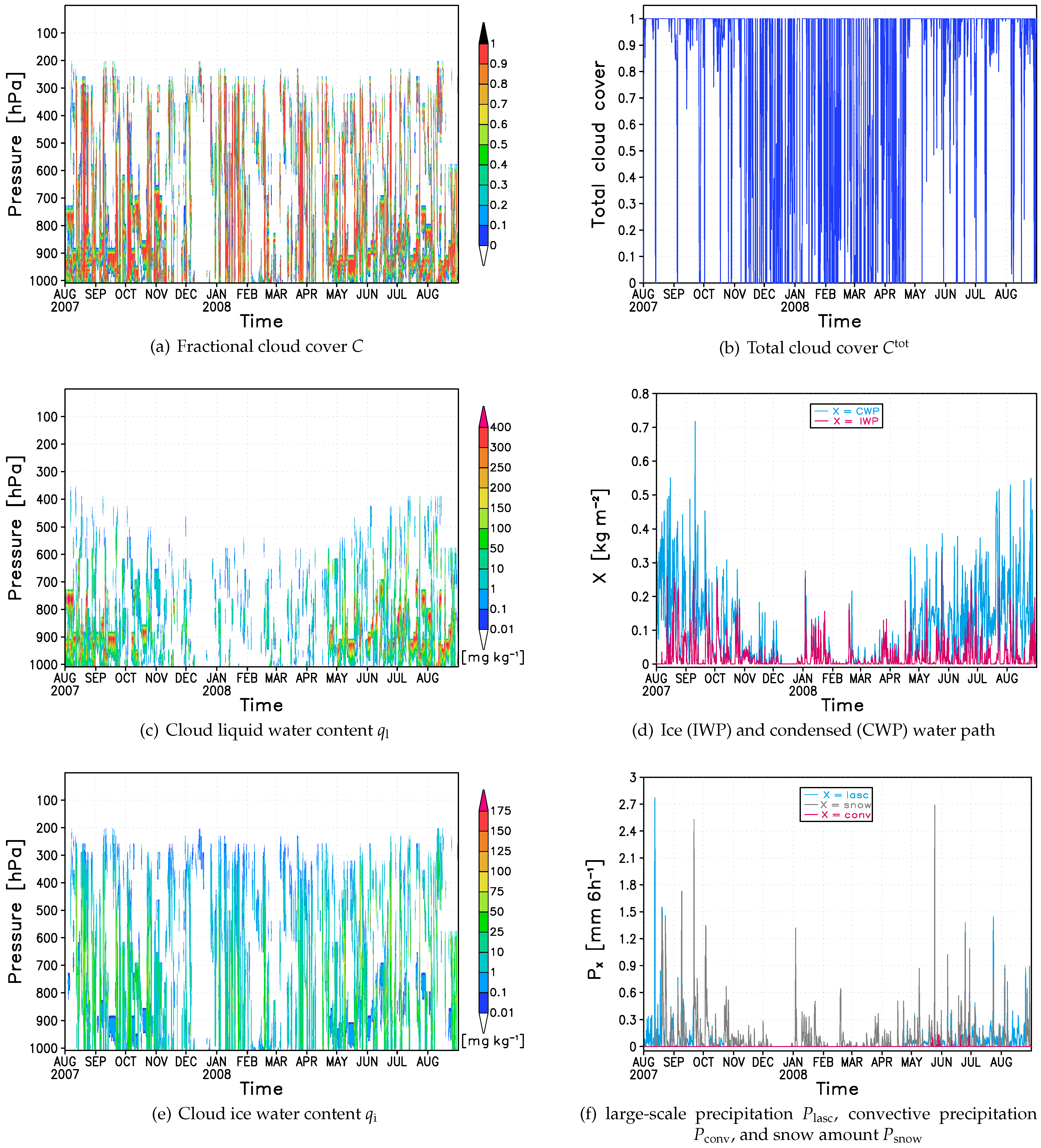
 ,
,  , condensed water path
  (sum of liquid and ice water paths), large-scale (stratiform)
  and convective
  precipitation, and additionally the snow amount
  with respect to total precipitation
  .
.
 ,
,  . In accordance to Intrieri et al. [15] Figure 3(c,e) show the more often occurrence of ice-only clouds during the WP than during the SP. While most of the simulated
  compared to mixed-phase clouds of the SP, which agrees with findings of Shupe and Intrieri [3]. Simulated
  (
(  (about 100km). From both data sets the observed cloud amount was extracted from August 2007 to August 2008. While ISCCP-D2 cloud amount corresponded to grid center coordinates of 106.36°E and 81.25°N, MODIS cloud amount was used with respect to a longitude of 103.0°E and latitude of 81.0°N, being the nearest-neighbor grid points to the start coordinates of NP-35 (102.81°E, 81.40°N).
 %) in the summer months and September but moderate cloudiness (fluctuating between 66.7% in January and 43.0% in March) during the rest of the year associated with distinct transitions starting in August 2007 and May 2008. This typical annual cycle of Arctic cloud cover has also been found in the satellite-based TOVS Polar Pathfinder data set ([71], not available after 2005) and ground-based observations by Hahn et al. [72]. In comparison to MODIS, ISCCP-D2 featured much more cloud cover from December to March (more than 30% higher in February) and less cloud cover during the rest of the year (more than 22% lower in August 2008), except for October. This leads to a reverse annual cycle in general, shifting the transition’s onsets to October (starting increase) and January (starting decrease). Apart from systematic and significant differences during the December–January–February season (highest RMSE of 23.8%) and March both satellite data sets at least produced same trends during the rest of the year. Further, ISCCP-D2 and MODIS agreed better during the summer period (SP) than during the winter period (WP), and the best statistical agreement appeared in the September–October–November season (lowest RMSE of 8.5%).
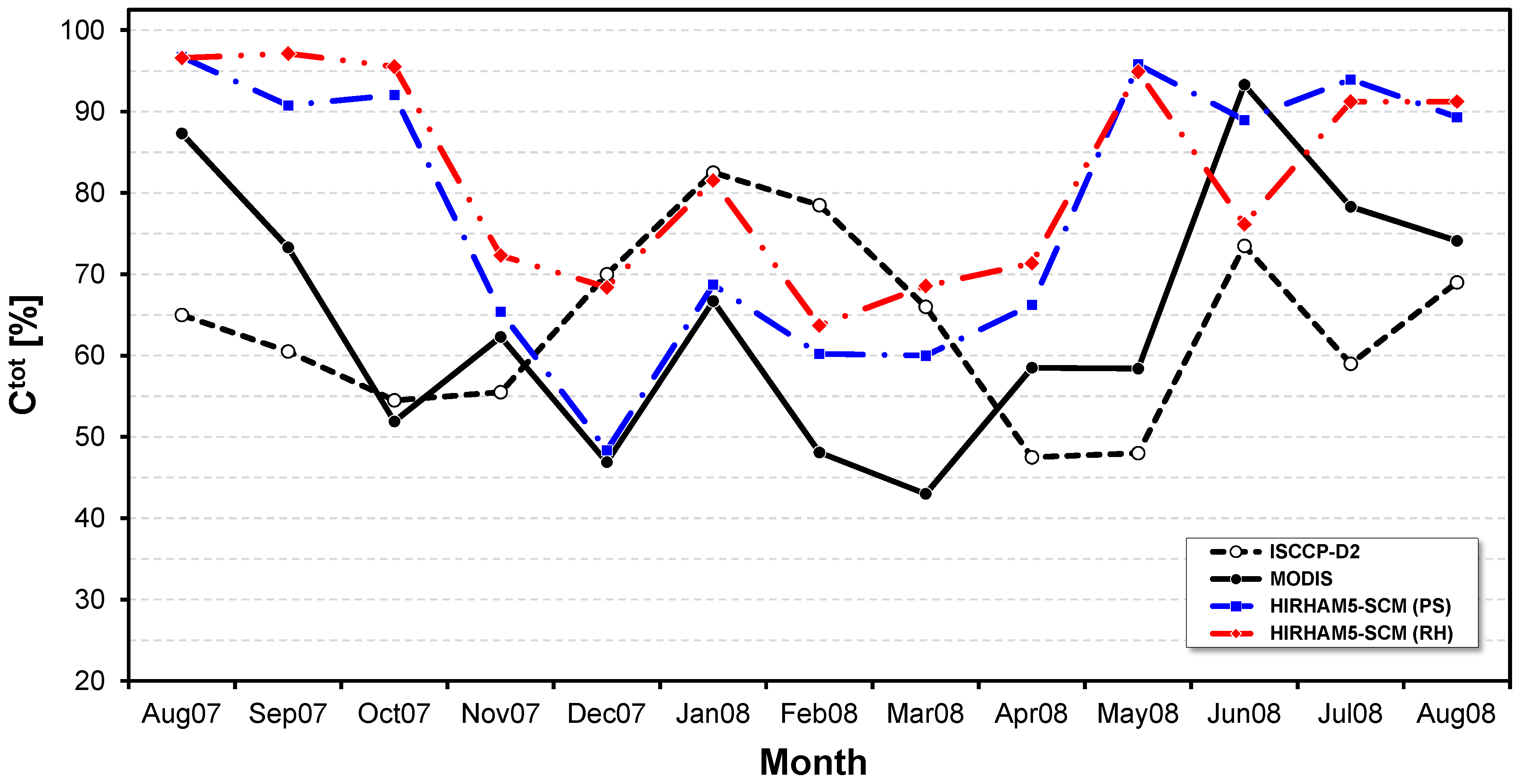
 ) were calculated for several cloud-related model variables both with respect to all 13 simulated months and the periods with moderate (WP) and high (SP)
  be the relative frequency of positive differences, then the percental decrease (
  ) or increase (
  ) of a certain model variable relative to the reference run can be computed using the formula
  . The results are listed in Table 4 and Table 5 either with respect to lower or higher tuning parameters.
 ,
,  ,
,  ,
,  ,
,  ,
,  ,
,  ,
,  ) relative to the default (Table 1) for the entire 13-month-long simulations (“all”) as well as the winter (WP) and summer (SP) periods as introduced in Section 3.2.1.


 , following the restrictions
  and
and  for the beta distribution shape parameters to obtain only unimodal distributions. Also according to Tompkins [45], the conditions
  and
and  were retained to exclude distributions with negative skewness.
 (left column) and one higher value of the tunable parameter
  and
and  . These sensitivity experiments were conducted at the NP-35 start position simulating from 1 August 2007 to 31 August 2008 by analogy to the reference run (Figure 3).
 . However, modifying this parameter only leads to temporary local changes of C (not shown), and overall
  reduction of
  and
and  (
(  ) but reduction of
  (
(  );
); rise in
  , and
, and 


 . Note that
  , which controls the conversion from (supercooled) cloud droplets to rain drops and thus the cloud lifetime effect, was found to be the next promising tuning parameter. This parameter was varied in the co-domain
  . Figure 6(a) and the sixth column of Table 4 and Table 5 confirm that only higher parameter values might be able to improve simulated cloudiness. Here, the increase in
  was identified as promising tuning parameter. This parameter controls the Bergeron–Findeisen process, which explains the growth of ice crystals at the expense of cloud droplets in mixed-phase clouds due to lower vapor pressures over ice than over water at subfreezing temperatures. Lohman et al. [66] have pointed out that as soon as the threshold of cloud ice content is exceeded a supercooled water cloud will glaciate immediately in the model. In the standard ECHAM5 code the remaining cloud water is not evaporated to deposit onto existing ice crystals but remaining cloud droplets have to either freeze or grow to precipitable sizes in subsequent time steps. For the sake of completeness
  . As shown by Figure 6(b) and the last column of Table 4 and Table 5, lower
  (left column) and one lower value of the tunable parameter
  and
and  . These sensitivity experiments were conducted at the NP-35 start position simulating from 1 August 2007 to 31 August 2008 by analogy to the reference run (Figure 3).

 ) and
) and  ) as well as lower
  ) and
) and  ) reduce simulated Arctic cloud cover, where the latter might be the most promising tuning parameter to improve cloud-related variables in the model.
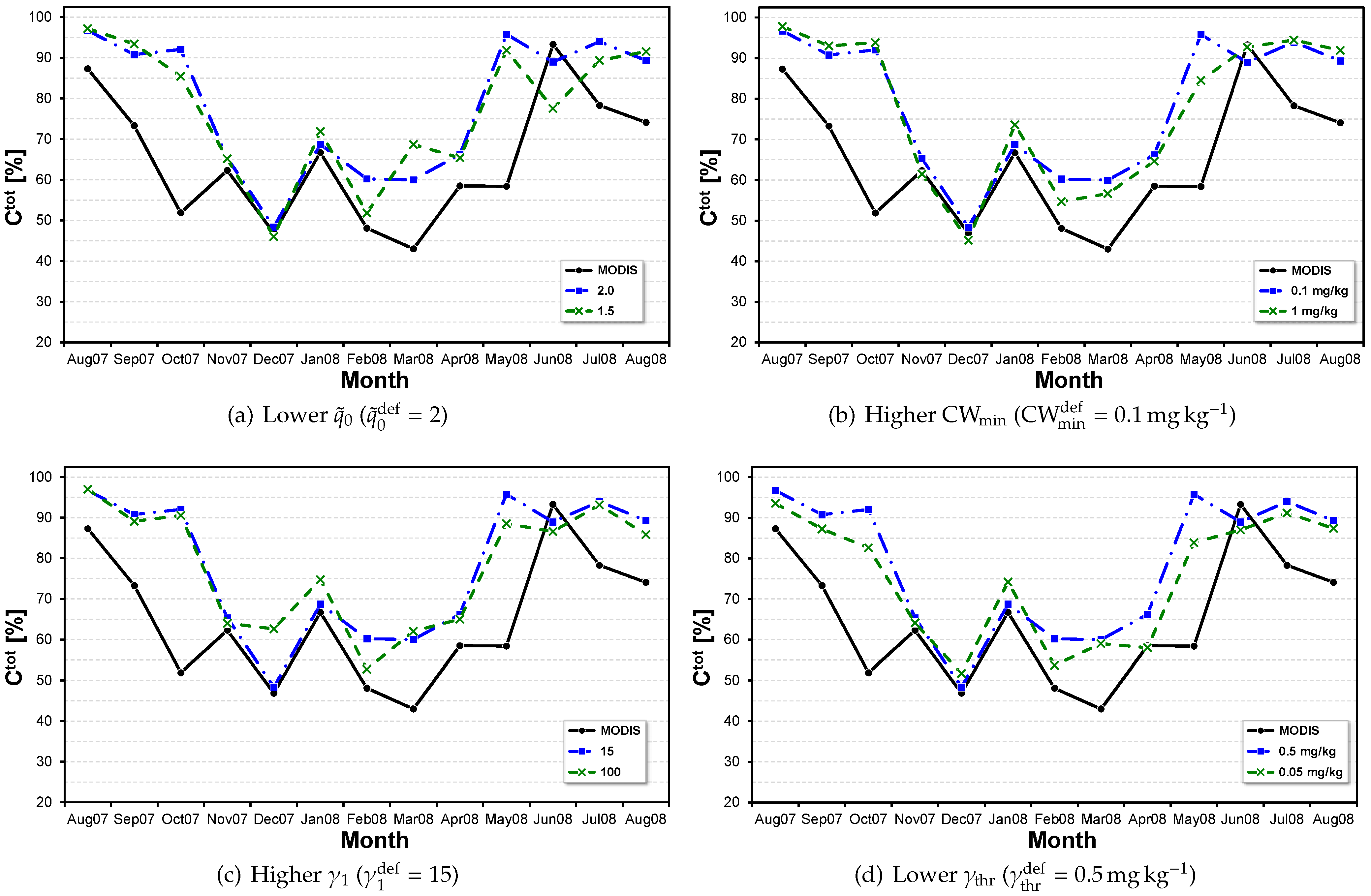


