Evaluation of Two Cloud Parameterizations and Their Possible Adaptation to Arctic Climate Conditions

Abstract

Based on the atmospheric regional climate model HIRHAM5, the single-column model version HIRHAM5-SCM was developed and applied to investigate the performance of a relative humidity based (RH-Scheme) and a prognostic statistical cloud scheme (PS-Scheme) in the central Arctic. The surface pressure as well as dynamical tendencies of temperature, specific humidity, and horizontal wind were prescribed from the ERA-Interim data set to enable the simulation of a realistic annual cycle. Both modeled temperature and relative humidity profiles were validated against radio soundings carried out on the 35th North Pole drifting station (NP-35). Simulated total cloud cover was evaluated with NP-35 and satellite-based ISCCP-D2 and MODIS observations. The more sophisticated PS-Scheme was found to perform more realistically and matched the observations better. Nevertheless, the model systematically overestimated the monthly averaged total cloud cover. Sensitivity studies were conducted to assess the effect of modified “tuning” parameters on cloud-related model variables. Two tunable parameters of the PS-Scheme and six tuning parameters contained in the cloud microphysics were analyzed. Lower values of the PS-Scheme adjustment parameter , which defines the shape of the symmetric beta distribution (acting as probability density function), as well as higher values of the cloud water threshold or autoconversion rate are able to reduce the overestimation of Arctic clouds. Furthermore, a lower cloud ice threshold , which controls the Bergeron–Findeisen process, improves model cloudiness and the ratio of liquid to solid water content.

2. Model Description

2.1. HIRHAM5-SCM Setup

The employed SCM is based on the three-dimensional atmospheric RCM HIRHAM5 [51], which comprises the dynamical core of the regional weather forecast model HIRLAM (HIgh Resolution Limited Area Model, [53]) and the physical parameterization package of the atmospheric general circulation model ECHAM5 (European Center Hamburg Model, [54]). HIRHAM5-SCM has 60 non-equidistant vertical levels, reaching from the surface up to a pressure height of 0.1h, where the lowermost 1 km is represented by approximately 10 levels. The levels are given in hybrid σ-p-coordinates following the ECMWF (European Center for Medium-Range Weather Forecasts) model level definitions by Berrisford et al. [55].

The hydrostatic model HIRHAM5 solves seven prognostic equations for the horizontal wind components u and v, temperature T, specific humidity q, cloud water content , cloud ice content , and surface pressure . The total tendency of a prognostic variable can be split into a physical (diabatic) and a dynamical (adiabatic) part, where the former describes temporal changes due to subgrid-scale processes like radiation, cloud formation, and vertical diffusion. HIRHAM5-SCM calculates physical tendencies explicitly, using an explicit Euler forward time stepping scheme with 10 min time step. Since the dynamical part cannot be computed by a SCM, HIRHAM5-SCM uses prescribed and dynamical tendencies of u, v, T and q in all model levels.

Dynamical tendencies, as resulting mainly from advection, play a fundamental role in controlling the evolution of the model state. Bergman and Sardeshmukh [56] have demonstrated that the consideration of dynamical tendencies leads to a dynamic stabilization of SCMs, avoiding the drift into non-physical states. In this study, dynamical tendencies were extracted from the most recent ECMWF reanalysis data set “ERA-Interim” (see [57]). This reanalysis provides 3-hourly total and physical tendencies of u, v, T, and q for recalculating the dynamical tendencies. It should be noted that advection of and could not be considered, since corresponding ERA-Interim tendencies are not available. The treatment of dynamical tendencies was similar to the method of “revealed forcing” as introduced by Randall and Cripe [58], but a nudging technique as explained by Lohmann et al. [59] was not applied. Further, ERA-Interim data was used for prescribing and the initialization of HIRHAM5-SCM.

The SCM-column was fixed in location during a single simulation, which always started at 0 UTC 1 August 2007 and mainly ran over 13 months to cover a whole annual cycle. In the present study, most of the model simulations were performed at the start coordinates of NP-35, which was located north of Severnaya Zemlya at 102.81°E longitude and 81.40°N latitude (figure with NP-35 track provided at [60]). For comparing model results with individual observations from NP-35 (see Section 3.1) the SCM-column was set to the position of the NP-35 trajectory at the time of the respective measurement. This means that both the initial values and the prescribed as well as dynamical tendencies were taken from the ERA-Interim grid point closest to the ice station at the time of the measurement. Since NP-35 measurements were carried out over a relatively large ice floe, all HIRHAM5-SCM runs used adapted, constant lower boundary conditions in terms of sea-ice fraction (100%), sea-ice thickness (2m), and sea-surface temperature (271.38 K). The latter represents the freezing point of sea water and was only used for calculating the conductive heat flux through the 2m thick sea-ice layer. The fixed 2m thickness of the modeled ice floe represents a reasonable approximation to the ice thicknesses measured at NP-35.

2.2. Cloud Cover Parameterizations

Since the main focus of this study was on Arctic clouds and due to the strong interaction between cloud and radiation processes, a brief introduction into the radiation and cloud cover parameterizations is given in the following.

The applied ECHAM5 parameterization package contains a scheme for the SW and LW radiation transfer, respectively [54]. In the longwave, the “Rapid Radiative Transfer Model” (RRTM) radiation code is used, which is based on the two-stream approximation. Apart from two modifications, the SW radiation code is the same as in the previous model version ECHAM4 [61]. First, the number of spectral bands has been doubled from two to four (two additional bands in the near-infrared) to avoid spurious absorption in clouds [62]. Second, transmissivities and reflectivities are separately calculated for the cloud-free and cloudy part of a grid box.

The scheme for the representation of stratiform clouds consists of three components: (1) prognostic equations for the vapor, liquid, and ice phase; (2) cloud microphysics according to Lohmann and Roeckner [43]; and (3) the PS-Scheme developed by Tompkins [45]. As an option within the model, the cloud cover scheme of the previous ECHAM4 version [61] can be chosen alternatively. This scheme is a RH-Scheme as formulated by Sundquist et al. [52]. Cloud microphysics considers precipitation formation by coalescence processes, aggregation of ice crystals to snow flakes, and accretion of cloud droplets by falling snow, as well as processes like gravitational sedimentation of ice crystals, evaporation of rain and sublimation of snow and ice, and also freezing of cloud liquid water and melting of cloud ice. Furthermore, phase changes between the water components due to condensation/evaporation and deposition/sublimation are considered.

In the RH-Scheme, fractional cloud cover C is derived from the diagnostic relation

(1)

where represents the grid box mean and the critical threshold of relative humidity. The latter decreases exponentially from 90% near the surface to 70% at higher altitudes (see [43]) and controls the onset of cloud formation.

In the PS-Scheme, subgrid-scale variability of total atmospheric water content is explicitly specified by a probability density function (PDF) in terms of the beta distribution . Note that defines the cloud condensate as sum of cloud water and cloud ice content. The scheme includes prognostic equations for the higher order moments of the beta distribution, namely variance (distribution width) and skewness, which are linked to subgrid-scale processes like turbulence, convection, and microphysics (see [45]). Fractional cloud cover is then computed as integral over the supersaturation part ( ) of the actual beta distribution:

(2)

where b is the upper bound of and denotes the saturation water content. defines the ratio of incomplete to complete beta function, where with the lower distribution bound , and and are the shape parameters of the beta distribution. Following Tompkins [45], the shape parameter is fixed in the model ( ). In contrast, , which is referred to as skewness parameter, is determined prognostically by

(3)

where the terms on the right-hand side refer to temporal changes due to turbulence, convection, and microphysical processes, respectively.

Finally, the total cloud cover is calculated by the model using a maximum-random overlap assumption with respect to computed values of C in the respective model levels. Clouds in contiguous layers are maximally overlapped, while clouds separated by one or more clear-sky layers are randomly overlapped.

The PS-Scheme includes the two adjustment parameters and K. The first parameter determines the shape of the symmetric beta distribution and appears in the turbulence term of the skewness equation

(4)

Here, and denote the vertical and horizontal mixing time scales (see [45]). While depends on the mixing length and the turbulent kinetic energy, is neglected since horizontal mixing is not available in the SCM version. Turbulent mixing processes due to subgrid-scale eddies mainly lead to a reduction of skewness and, therefore, to an aspiration towards a symmetric beta distribution. Currently, is used as default value, restricting the skewness of to a co-domain of .

The second adjustment parameter K, which is set to the default value of , appears in the convection term of the skewness equation

(5)

and specifies how fast the skewness of the beta distribution increases according to the detrainment of cloud condensate due to cumulus convection. In Equation (5), is the mean air density and represents the mass flux of cloud condensate due to convective updraft, where denotes the updraft mass flux and the mean cloud condensate inside the updraft, assuming that . The superscript “cu” denotes that the respective variables are calculated by the cumulus convection scheme, which is based on the mass flux scheme of Tiedtke [63] with modifications for penetrative convection according to Nordeng [64].

In addition, model parameters contained in the cloud microphysics were analyzed, since they have a direct influence on cloud formation and dissipation. One of these parameters is the minimum cloud water content , which avoids negative and , and which is additionally a threshold for the existence of clouds in the PS-Scheme. If the grid box means of cloud liquid and cloud ice content fulfill and , C will be set to zero. Thus, clouds will only appear in the PS-Scheme if at least one of the two variables exceeds . The default value of was used in accordance to Zhang and Lohmann [49].

An overview on the modified model parameters is given in Table 1 (for equations and further details see Roeckner et al. [54]).

Table 1. Notation, default value, regarded parameter range (co-domain), and description of modified model tuning parameters. Apart from , which is not mentioned by Roeckner et al. [54], the notation conforms to the ECHAM5 documentation.

Parameter	Default	Co-domain	Description (Meaning)
	2		determines the shape of the symmetric beta distribution, which is used as PDF in the PS-Scheme
K	10		determines the efficiency of convective detrainment to increase the skewness of the beta distribution
			avoids negative cloud water and ice contents and additionally controls the occurrence of clear-sky conditions in the PS-Scheme
	15		determines the efficiency of rain drop formation by collision and coalescence of cloud drops (autoconversion rate)
	5		determines the efficiency of rain drop growth by collision and coalescence with cloud drops as well as the efficiency of snow flake growth by aggregation of surrounding ice particles
	95		determines the efficiency of snow formation by aggregation of cloud ice particles (aggregation rate)
	0.1		determines the accretion rate of ice crystals by supercooled cloud drops (growth of snow crystals) through colliding and coalescing with them (riming)
			cloud ice threshold, which determines the efficiency of the Bergeron–Findeisen process

Table 1. Notation, default value, regarded parameter range (co-domain), and description of modified model tuning parameters. Apart from , which is not mentioned by Roeckner et al. [54], the notation conforms to the ECHAM5 documentation.

Parameter	Default	Co-domain	Description (Meaning)
	2		determines the shape of the symmetric beta distribution, which is used as PDF in the PS-Scheme
K	10		determines the efficiency of convective detrainment to increase the skewness of the beta distribution
			avoids negative cloud water and ice contents and additionally controls the occurrence of clear-sky conditions in the PS-Scheme
	15		determines the efficiency of rain drop formation by collision and coalescence of cloud drops (autoconversion rate)
	5		determines the efficiency of rain drop growth by collision and coalescence with cloud drops as well as the efficiency of snow flake growth by aggregation of surrounding ice particles
	95		determines the efficiency of snow formation by aggregation of cloud ice particles (aggregation rate)
	0.1		determines the accretion rate of ice crystals by supercooled cloud drops (growth of snow crystals) through colliding and coalescing with them (riming)
			cloud ice threshold, which determines the efficiency of the Bergeron–Findeisen process

3. Evaluation of Two Cloud Cover Schemes

3.1. Evaluation with NP-35 Measurements

To evaluate the performance of HIRHAM5-SCM, a series of case studies was conducted, and then model results were compared with NP-35 measurements carried out from middle of October 2007 to the beginning of April 2008. For the comparison with an individual measurement, a single model run (from 0 UTC 1 August 2007 to the time of the measurement) was performed, respectively and during model start the SCM-column was set to the corresponding position of NP-35 according to Table 2 (as explained in Section 2.1). On the one hand, simulated vertical profiles of temperature T and relative humidity RH were checked against NP-35 radio soundings, which were started twice a day at 0 UTC and 12 UTC. 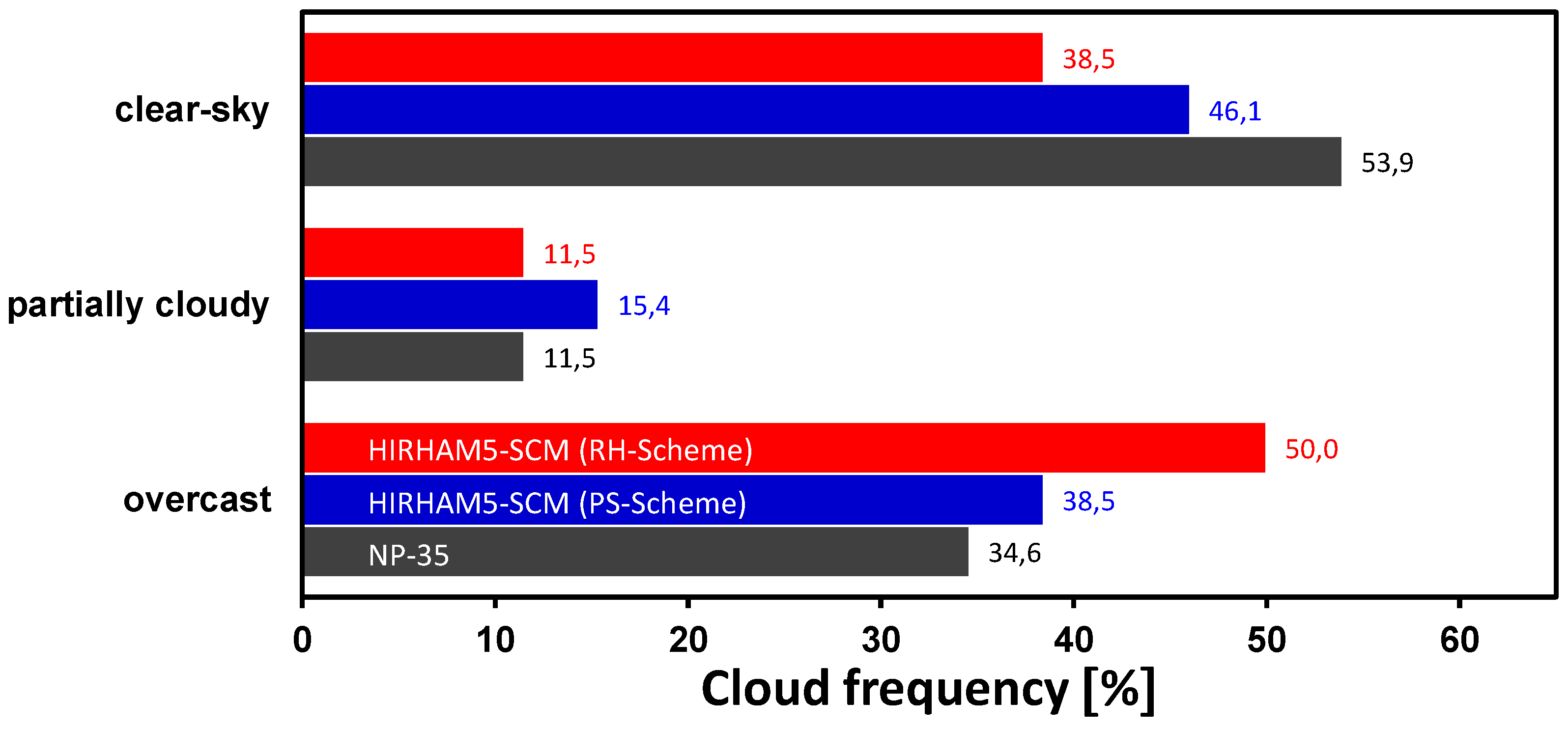On the other hand, modeled and observed total cloud cover were compared, where the latter was available from 6-hourly NP-35 weather reports.

Except for April 2008, where the first radio sounding was available on 2 April and the last available radiosonde was started on 7 April, the 1st and 15th of a respective month at midnight and midday were chosen for the evaluation (see Table 2). Exemplarily, Figure 1 shows observed and modeled height profiles of T and RH, and additionally modeled fractional cloud cover C at three specific events.

3.1.1. Three Specific Cases

To illustrate the different performance of RH-Scheme and PS-Scheme, three cases associated with totally overcast (0 UTC 1 November 2007), clear-sky (12 UTC 15 January 2008), and partially cloudy (0 UTC 2 April 2008) conditions with respect to observed (see Table 2) were chosen.

Table 2. Listed are the geographic location (Longitude, Latitude) of the SCM-column for conducted case studies corresponding to the respective NP-35 radiosonde ascent and both observed and modeled total cloud cover using either the PS-Schem or RH-Scheme. In the notation “yyyy-mm-dd_hh”, “yyyy” = year, “mm” = month, “dd” = day and “hh” = hour. Dates in bold type are discussed in detail in Section 3.1.1.

Date	Lon(°E)	Lat(°N)	(%)
			NP-35	SCM(PS)	SCM(RH)
2007-10-15_00	101.86	81.60	100.0	89.6	100.0
10-15_12	102.22	81.56	100.0	100.0	100.0
11-01_00	102.06	82.42	100.0	100.0	100.0
11-01_12	101.86	82.40	0.0	64.6	100.0
11-15_00	97.52	82.10	0.0	0.0	0.0
11-15_12	97.55	82.11	0.0	100.0	100.0
12-01_00	97.56	83.02	0.0	100.0	100.0
12-01_12	97.31	82.99	100.0	100.0	100.0
12-15_00	97.69	83.40	0.0	0.0	0.0
12-15_12	97.92	83.45	0.0	0.0	0.0
2008-01-01_00	92.49	84.75	0.0	0.0	100.0
01-01_12	92.32	84.73	0.0	0.0	0.0
01-15_00	91.82	85.06	0.0	100.0	100.0
01-15_12	91.13	85.04	0.0	100.0	100.0
02-01_00	78.12	85.17	0.0	100.0	100.0
02-01_12	77.98	85.15	100.0	100.0	100.0
02-15_00	71.51	85.65	100.0	100.0	84.9
02-15_12	71.31	85.64	100.0	0.0	0.0
03-01_00	61.16	85.52	100.0	58.1	79.8
03-01_12	60.97	85.50	0.0	0.0	0.0
03-15_00	55.96	85.52	0.0	0.0	100.0
03-15_12	60.98	85.50	25.0	0.0	0.0
04-02_00	42.23	84.75	87.5	0.0	45.8
04-02_12	42.22	84.71	12.5	15.0	0.0
04-07_00	42.21	84.29	100.0	0.0	0.0
04-07_12	41.90	84.27	0.0	0.0	0.0

Table 2. Listed are the geographic location (Longitude, Latitude) of the SCM-column for conducted case studies corresponding to the respective NP-35 radiosonde ascent and both observed and modeled total cloud cover using either the PS-Schem or RH-Scheme. In the notation “yyyy-mm-dd_hh”, “yyyy” = year, “mm” = month, “dd” = day and “hh” = hour. Dates in bold type are discussed in detail in Section 3.1.1.

Date	Lon(°E)	Lat(°N)	(%)
			NP-35	SCM(PS)	SCM(RH)
2007-10-15_00	101.86	81.60	100.0	89.6	100.0
10-15_12	102.22	81.56	100.0	100.0	100.0
11-01_00	102.06	82.42	100.0	100.0	100.0
11-01_12	101.86	82.40	0.0	64.6	100.0
11-15_00	97.52	82.10	0.0	0.0	0.0
11-15_12	97.55	82.11	0.0	100.0	100.0
12-01_00	97.56	83.02	0.0	100.0	100.0
12-01_12	97.31	82.99	100.0	100.0	100.0
12-15_00	97.69	83.40	0.0	0.0	0.0
12-15_12	97.92	83.45	0.0	0.0	0.0
2008-01-01_00	92.49	84.75	0.0	0.0	100.0
01-01_12	92.32	84.73	0.0	0.0	0.0
01-15_00	91.82	85.06	0.0	100.0	100.0
01-15_12	91.13	85.04	0.0	100.0	100.0
02-01_00	78.12	85.17	0.0	100.0	100.0
02-01_12	77.98	85.15	100.0	100.0	100.0
02-15_00	71.51	85.65	100.0	100.0	84.9
02-15_12	71.31	85.64	100.0	0.0	0.0
03-01_00	61.16	85.52	100.0	58.1	79.8
03-01_12	60.97	85.50	0.0	0.0	0.0
03-15_00	55.96	85.52	0.0	0.0	100.0
03-15_12	60.98	85.50	25.0	0.0	0.0
04-02_00	42.23	84.75	87.5	0.0	45.8
04-02_12	42.22	84.71	12.5	15.0	0.0
04-07_00	42.21	84.29	100.0	0.0	0.0
04-07_12	41.90	84.27	0.0	0.0	0.0

Figure 1(a) reveals high C on 1 November 2007 independent from the used cloud scheme, where low- (below 700h), mid- (700 to 400 h), and high-level (above 400h) clouds were simulated. While the RH-Scheme produced a totally overcast sky below 810h, the PS-Scheme showed pressure ranges with alternating clear-sky and overcast conditions. In the middle troposphere the PS-Scheme simulated an overcast sky around 710h, whereas the RH-Scheme produced one low-level and mid-level cloud layer around 761h and 576h, respectively associated with partial cloudiness. The vertical cloud structures were very similar above 500h, but the RH-Scheme simulated up to 35% higher absolute values. On 1 November 2007 polar night has already prevailed (at current NP-35 position, see Table 2) so that Arctic clouds can be associated with near-surface warming independent from cloud family due to the absence of SW CRF. Thus, the enhanced cloudiness simulated by the RH-Scheme leads to higher temperatures in the near-surface layer and allows for a better match to the observation, which is confirmed by near-surface temperature differences of -2.3K (PS-Scheme) and -0.8K (RH-Scheme), respectively. On the other hand, the PS-Scheme is better able to model the linkage between the occurrence of Arctic stratus clouds and capping strong temperature inversion as well as rapid moisture decrease (e.g., 882 to 855 h). Nevertheless, this linkage does not always agree with the observation (e.g., 690 to 653 h). 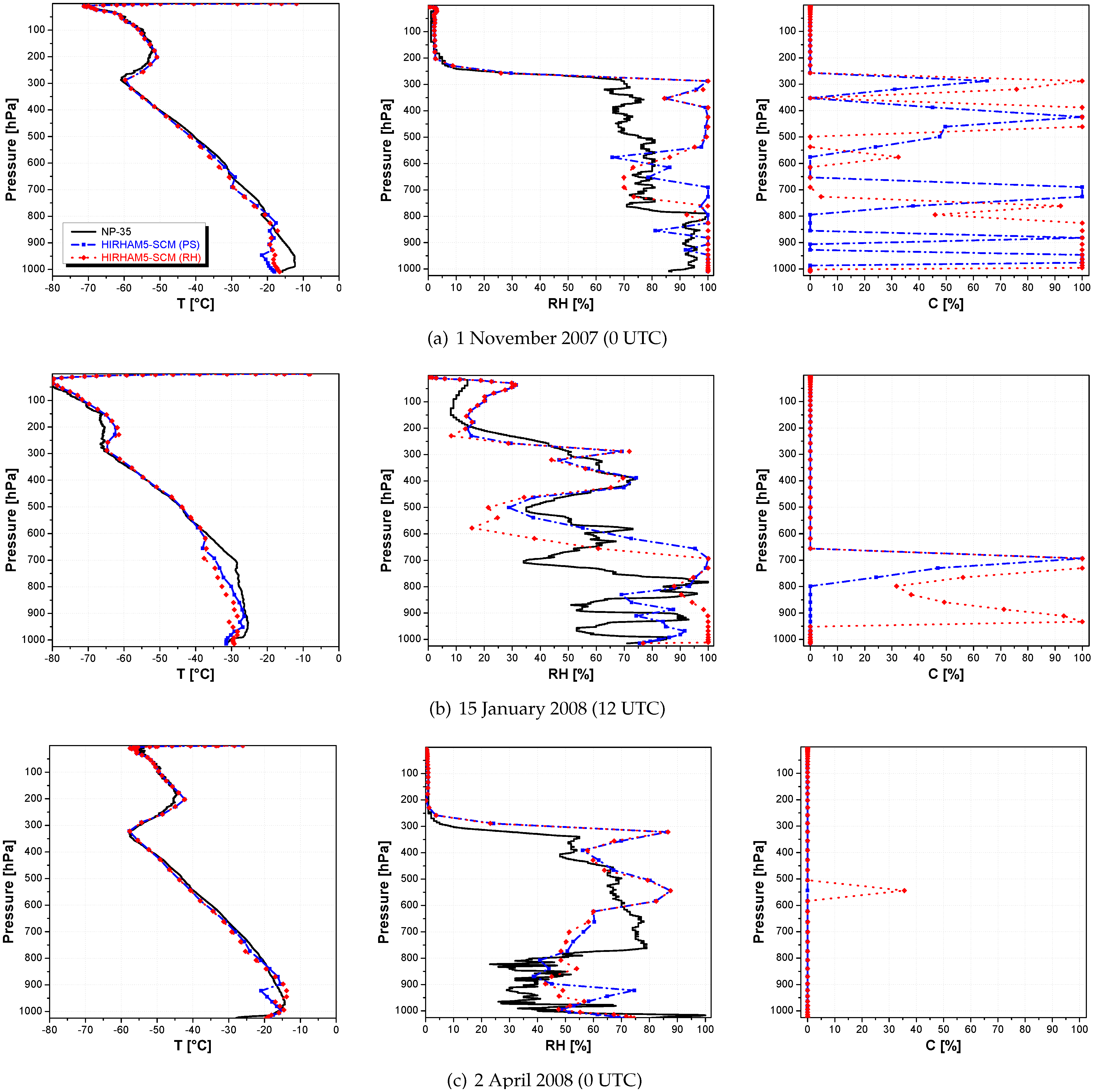In agreement with the NP-35 observation both cloud schemes produced a of 100% (cf. Table 2).

On 15 January 2008 (Figure 1(b)) the RH-Scheme produced two overcast cloud decks around 933h and 693h, respectively with partially cloudy conditions in between. In contrast, the PS-Scheme simulated only the upper-level cloud deck. While the PS-Scheme matches the observed RH-profile much better between 450 to 610 h and from 800h to the surface, modeled profiles of RH are almost identical and in part accurately agree with the measurement (e.g., 360 to 440 h). The RH-Scheme overestimates measured RH significantly (up to 47%) from 1,012 h to 830h, leading to more BLCs associated with enhanced LW CRF and 2.2K higher near-surface temperatures relative to the PS-Scheme. Although both cloud schemes consistently produced low-level clouds and also the same of 100%, this totally differs from the observed clear sky. Since the PS-Scheme simulated less clouds below 600h, it likely matches the observed T-profile better in the ABL, but the actual temperature structure is of course also determined by other processes like turbulent vertical heat exchange and cannot be explained only by the effect of CRF.

Figure 1. Vertical profiles of temperature T (in °C) (left column), relative humidity RH (in %) (middle column), and fractional cloud cover C (in %) (right column) at various dates, originating from NP-35 radiosonde ascents (black curves) and HIRHAM5-SCM simulations using either the PS-Scheme (blue curves) or RH-Scheme (red curves).

Figure 1. Vertical profiles of temperature T (in °C) (left column), relative humidity RH (in %) (middle column), and fractional cloud cover C (in %) (right column) at various dates, originating from NP-35 radiosonde ascents (black curves) and HIRHAM5-SCM simulations using either the PS-Scheme (blue curves) or RH-Scheme (red curves).

Contrary to the cases before, on 2 April 2008 (Figure 1(c)) only the RH-Scheme produced fractional cloud cover around 544h, while both modeled RH-profiles were almost identical here and also above. Overall, the RH-Scheme produced a of 45.8% implying a much smaller difference (41.7%) to the observed NP-35 value. Significant differences between the two simulated profiles of RH occurred in the pressure range from 623h to 964h, where the PS-Scheme agrees better with the NP-35 observation between 623 to 897 h but worse between 897 to 964 h. The two modeled temperature structures were very similar above 897h matching the observation fairly well. Although the RH-Scheme simulated some mid-level clouds, the measured strong ground-based temperature inversion is as underestimated as by the PS-Scheme (about 9K too warm inversion base). Partial cloudiness produced by the RH-Scheme improves the simulated temperature profile between 897 to 964 h, but the consistently modeled elevated temperature inversion starting in 963h (RH-Scheme) and 922h (PS-Scheme), respectively totally disagrees with the measurement. The NP-35 radiosonde ascent showed 100% RH around 1,016h and low near-surface temperatures of -28.7°C arguing for a low-level cloud deck associated with dominant SW CRF (enhanced cloud albedo effect), which could not be reproduced by the model.

Wang et al. [65] have demonstrated that the surface temperature is higher in the presence of multi-layered Arctic clouds than in cases of single-layer BLCs. This finding is in accordance to Figure 1(b). LW radiative cooling at the cloud top generates energetic turbulent eddies which effectively transport the radiatively cooled air down to the ground, except for the storm-driven cloudy ABL [29]. This effect is most likely overestimated by the model (as suggested in Figure 1(a,b)) favoring condensation or resublimation which finally leads to enhanced cloud formation. While deviations between modeled T- and RH-profiles are generally small in case of similar cloud profiles, they become significant as soon as the two cloud schemes simulate different vertical cloud structures. Although both cloud schemes sometimes model almost the same T- and RH-profiles, they can significantly differ from the observation especially in the ABL. Even when complete absence of model clouds is consistently produced in the entire SCM-column (not shown), simulated T- and RH-profiles either can differ from each other or do not agree with the observation. In general, the more pronounced vertical variability of moisture cannot be reproduced accurately by the model. Thus, the RH-Scheme a priori produces clouds at incorrect altitudes.

3.1.2. Statistics over All Cases

To validate simulated profiles of T and RH quantitatively for the 26 studied cases, the Pearson product-moment correlation (autocorrelation) coefficient was computed in every model level with respect to NP-35 measurements. Since none of the studied NP-35 radiosondes rose higher than 7h and at least two radiosonde measurements should be available for a certain pressure height, could only be calculated for the 48 uppermost model levels (lowermost altitudes), where the 13th model level is situated in about 8h (32 km height).

For temperature, solely positive and high correlation coefficients ( ) were calculated within the entire atmospheric column independently from the applied cloud scheme. While the temperature correlation was consistently very high ( ) above the 30th model level (about 200h), the strength of the linear relation decreased below and became minimal in the ABL. This was confirmed by vertically averaged correlation coefficients computed either for the entire SCM-column or the 10 model levels closest to the surface. While the PS-Scheme produced (13 to 60 model level) and (51 to 60 model level), the RH-Scheme showed slightly lower mean correlations of 0.94 and 0.85, respectively. HIRHAM5-SCM generally produced comparably low temperature correlations in the three model levels closest to the surface ( for RH-Scheme) indicating incorrect turbulent heat fluxes. Interestingly, lowest values of (up to 0.76) appeared around the 52nd model level (about 930h), which might be explained with an incorrect coupling between ABL and the free troposphere in the model. The RH-Scheme produced slightly higher correlation coefficients between the 51st (about 910h) and 54th (about 965h) model level but otherwise the PS-Scheme produced either equal or higher correlations. Overall, the PS-Scheme therefore correlates better with measured NP-35 profiles of T.

Correlation coefficients of relative humidity were mainly high ( ) above the 38th model level (about 460h). As compared with the correlation coefficients of RH were also positive but decreased faster with increasing model level (decreasing altitude) and rarely dropped below 0.4 up to the 56th model level (around 990h). In contrast, the four model levels closest to the surface were associated with low correlation coefficients ( ) and were even negative in case of the RH-Scheme. Negative correlation coefficients in the near-surface layer indicate more serious problems in correctly simulating ground-based temperature inversions leading to incorrect vertical moisture fluxes. The vertically averaged correlation coefficients with respect to the entire atmospheric column (0.70 and 0.68 for PS-Scheme and RH-Scheme, respectively) and the ABL (0.33 and 0.29 for PS-Scheme and RH-Scheme, respectively) confirmed that the model has more serious difficulties in accurately simulating the ABL, but also that the PS-Scheme correlates better with measured NP-35 profiles of RH.

For further validating the applied cloud schemes against NP-35, relative frequencies of clear-sky, partially cloudy, and (totally) overcast cases were calculated. Figure 2 reveals that clear-sky conditions prevailed in more than half the observations, slightly more than one third represented overcast conditions, and only in slightly more than one ninth of the cases partial cloudiness was observed.

Figure 2. Relative frequencies of clear-sky, partially cloudy, and overcast cases based on all 26 conducted case studies (Table 2), shown for NP-35 observations and model simulations using either the PS-Scheme or RH-Scheme.

Figure 2. Relative frequencies of clear-sky, partially cloudy, and overcast cases based on all 26 conducted case studies (Table 2), shown for NP-35 observations and model simulations using either the PS-Scheme or RH-Scheme.

On the one hand, the RH-Scheme agrees with the observed frequency of partially cloudy cases (11.5%), while about 4% more cases are produced by the PS-Scheme. On the other hand, the model underestimates clear-sky cases by 7.8% (PS-Scheme) and 15.4% (RH-Scheme) but overestimates overcast cases by 3.9% (PS-Scheme) and 15.4% (RH-Scheme). Overall, HIRHAM5-SCM overestimates cloudy cases (sum of partially cloudy and overcast cases) by the same percentages as for the underestimation of clear-sky cases and therefore, the PS-Scheme matches NP-35 observations much better.

3.2. Arctic Clouds in the Reference Run

Starting point for the sensitivity studies in Section 4 was a reference run that uses the standard configuration of the model (usage of default model parameters). Here, a single HIRHAM5-SCM reference run (from 1 August 2007 to 31 August 2008) was conducted for both the PS-Scheme and RH-Scheme.

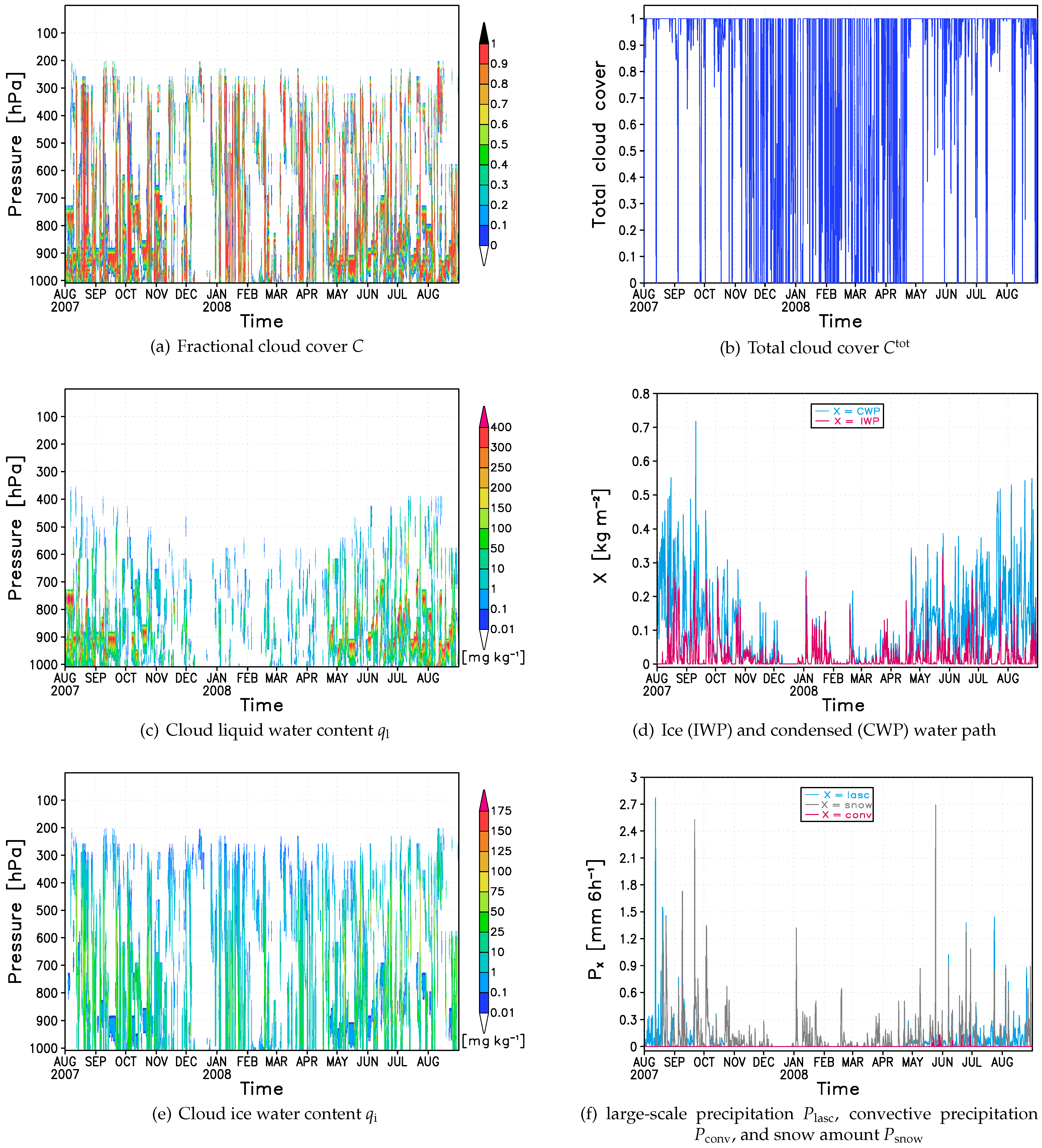
3.2.1. Annual Cycle of Cloud-Related Variables

Applying the PS-Scheme, Figure 3 shows time-height cross sections of , , and as well as the temporal evolution of , ice water path , condensed water path (sum of liquid and ice water paths), large-scale (stratiform) and convective precipitation, and additionally the snow amount with respect to total precipitation .

Figure 3(a,b) reveal rather moderate cloudiness during the WP (winter period: from mid-November 2007 to mid-April 2008; i.e., predominantly polar night) associated with strong fluctuations between (totally) overcast (49.7%) and clear-sky (31.6%) conditions. On the other hand, the PS-Scheme produced enhanced cloudiness during the SP (summer period: entire modeled time range except for WP; i.e., predominantly polar day), where an overcast sky (75.3%) occurred more often than a clear sky (5.0%). In particular, low-level clouds (below 700h) appeared more often during summer and autumn in accordance to the frequently observed presence of summertime BLCs (e.g., [14]). Inoue et al. [29] have found one possible mechanism for the layered structure of summertime BLCs, which depends on the combination of shear mixing near the surface and radiative cooling at the cloud top in the storm-driven cloudy ABL. The RH-Scheme behaved similar during the SP (not shown), but overall, this cloud scheme tends to simulate larger cloud amounts in general (confirmed by Section 3.2.2). In fact, during the SP an overcast sky (77.4%) occurred also more often than a clear sky (4.7%), while the RH-Scheme produced much more cases with overcast conditions (about 10% more than PS-Scheme) but less cases with clear-sky conditions (about 3% less than PS-Scheme) during the WP. The latter is basically the same result as obtained from the comparison with NP-35 (see Section 3.1.2).

In the PS-Scheme subgrid-scale sources and sinks of clouds directly control the temporal evolution of the cloud representing area below the beta distribution (see Section 2.2), and thus more realistic model cloudiness can be achieved as demonstrated by Tompkins [45]. An advanced feature is therefore the ability to simulate abrupt changes from totally overcast to clear-sky conditions (e.g., between 0 UTC and 6 UTC 13 August 2007 in Figure 3(b)) and vice versa (e.g., between 12 UTC and 18 UTC 13 August 2007 in Figure 3(b)), which were also apparent in NP-35 weather reports (not shown). The simulation of such abrupt changes in happened less often and rather randomly when using the RH-Scheme, because the subgrid-scale variability of water vapor is only indirectly considered by the threshold of relative humidity, and the linkage to cloud formation and dissipation processes is missing.

Figure 3. Simulated fractional (a) and total (b) cloud cover, cloud liquid (c) and ice (e) water content, ice and condensed (sum of liquid and ice water paths) water path (d) as well as large-scale and convective precipitation and the contribution of snow (f) for the period from 1 August 2007 to 31 August 2008. This HIRHAM5-SCM reference run was conducted at the NP-35 start position (102.81°E, 81.40°N) using the PS-Scheme and applying default model parameters (see Table 1). The results are shown as 6-hourly standard model output.

Figure 3. Simulated fractional (a) and total (b) cloud cover, cloud liquid (c) and ice (e) water content, ice and condensed (sum of liquid and ice water paths) water path (d) as well as large-scale and convective precipitation and the contribution of snow (f) for the period from 1 August 2007 to 31 August 2008. This HIRHAM5-SCM reference run was conducted at the NP-35 start position (102.81°E, 81.40°N) using the PS-Scheme and applying default model parameters (see Table 1). The results are shown as 6-hourly standard model output.

HIRHAM5-SCM produced a reasonable annual cycle of , , , and . In accordance to Intrieri et al. [15] Figure 3(c,e) show the more often occurrence of ice-only clouds during the WP than during the SP. While most of the simulated was located below 700h, significant amounts of were still modeled above 500h. Figure 3(d) reveals that wintertime Arctic mixed-phase clouds can be associated with lower compared to mixed-phase clouds of the SP, which agrees with findings of Shupe and Intrieri [3]. Simulated and had also the correct order of magnitude (e.g., [28]). was dominated by except for June and July 2008, where was generated as well (Figure 3(f)). During the SP much higher was modeled than during the WP, where the latter period was more dominated by .

Lohmann et al. [66] have shown that the stand-alone ECHAM5 GCM overestimates ( ) but underestimates ( ), and they have found an overestimation of ( ) as well as . Microphysical cloud characteristics from NP-35 are not available. Hence, these findings were qualitatively examined by comparison with observations carried out during the Surface Heat Budget of the Arctic Ocean (SHEBA, October 1997–1998). Our results (not shown) suggested a similar behavior in HIRHAM5-SCM as mentioned by Lohmann et al. [66].

3.2.2. Evaluation with Satellite Observations

On the one hand, the advanced International Satellite Cloud Climatology Project data set ISCCP-D2 [67] was used to evaluate the simulated monthly averaged . ISCCP-D2 cloud data refer to an equal-area grid with horizontal resolution of about 280km and is provided at [68]. The second satellite-based data set originated from the Moderate Resolution Imaging Spectroradiometer (MODIS) “MOD08_M3-Level3 Monthly Joint Aerosol Vapor/Cloud Product” described by Hubanks et al. [69]. This “Terra Atmosphere Level 3 Product” (Collection 5; [70]) provides a horizontal resolution of (about 100km). From both data sets the observed cloud amount was extracted from August 2007 to August 2008. While ISCCP-D2 cloud amount corresponded to grid center coordinates of 106.36°E and 81.25°N, MODIS cloud amount was used with respect to a longitude of 103.0°E and latitude of 81.0°N, being the nearest-neighbor grid points to the start coordinates of NP-35 (102.81°E, 81.40°N).

First, Figure 4 reveals a qualitative disagreement between the annual cycles of ISCCP-D2 and MODIS, which was quantitatively confirmed by a relatively large overall root mean square error (RMSE of all 13 months) of 17.5% listed in Table 3. MODIS featured enhanced cloudiness ( %) in the summer months and September but moderate cloudiness (fluctuating between 66.7% in January and 43.0% in March) during the rest of the year associated with distinct transitions starting in August 2007 and May 2008. This typical annual cycle of Arctic cloud cover has also been found in the satellite-based TOVS Polar Pathfinder data set ([71], not available after 2005) and ground-based observations by Hahn et al. [72]. In comparison to MODIS, ISCCP-D2 featured much more cloud cover from December to March (more than 30% higher in February) and less cloud cover during the rest of the year (more than 22% lower in August 2008), except for October. This leads to a reverse annual cycle in general, shifting the transition’s onsets to October (starting increase) and January (starting decrease). Apart from systematic and significant differences during the December–January–February season (highest RMSE of 23.8%) and March both satellite data sets at least produced same trends during the rest of the year. Further, ISCCP-D2 and MODIS agreed better during the summer period (SP) than during the winter period (WP), and the best statistical agreement appeared in the September–October–November season (lowest RMSE of 8.5%).

Figure 4. Monthly means of total cloud cover (in %) from August 2007 to August 2008 referring to the NP-35 start position. The results originate from both ISCCP-D2 (short dashed black line) and MODIS (solid black line) satellite observations, and HIRHAM5-SCM simulations using either the PS-Scheme (blue line) or the RH-Scheme (red line).

Figure 4. Monthly means of total cloud cover (in %) from August 2007 to August 2008 referring to the NP-35 start position. The results originate from both ISCCP-D2 (short dashed black line) and MODIS (solid black line) satellite observations, and HIRHAM5-SCM simulations using either the PS-Scheme (blue line) or the RH-Scheme (red line).

Table 3. Root mean square errors (RMSEs) of monthly averaged (in %) (based on Figure 4) for the satellite data sets among each other and in comparison with the HIRHAM5-SCM reference simulation using either the PS-Scheme or RH-Scheme.

		RMSE(%)
		ISCCP-D2	MODIS	SCM(PS-Scheme)	SCM(RH-Scheme)
SON	ISCCP-D2	—	8.5	28.4	33.2
	MODIS	8.5	—	25.3	29.3
DJF	ISCCP-D2	—	23.8	18.2	8.6
	MODIS	23.8	—	7.1	17.6
MAM	ISCCP-D2	—	15.9	29.8	30.4
	MODIS	15.9	—	24.1	26.8
JJA	ISCCP-D2	—	16.2	25.0	22.6
	MODIS	16.2	—	12.9	15.9
WP	ISCCP-D2	—	20.0	15.7	13.4
	MODIS	20.0	—	9.2	17.5
SP	ISCCP-D2	—	15.0	32.7	33.3
	MODIS	15.0	—	23.6	25.8
all months	ISCCP-D2	—	17.5	26.3	26.1
	MODIS	17.5	—	18.4	22.3

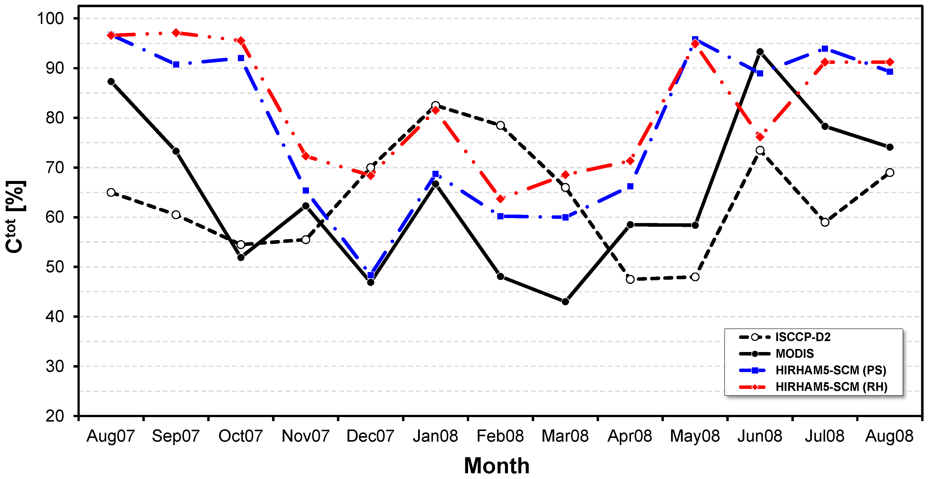Table 3. Root mean square errors (RMSEs) of monthly averaged (in %) (based on Figure 4) for the satellite data sets among each other and in comparison with the HIRHAM5-SCM reference simulation using either the PS-Scheme or RH-Scheme.

		RMSE(%)
		ISCCP-D2	MODIS	SCM(PS-Scheme)	SCM(RH-Scheme)
SON	ISCCP-D2	—	8.5	28.4	33.2
	MODIS	8.5	—	25.3	29.3
DJF	ISCCP-D2	—	23.8	18.2	8.6
	MODIS	23.8	—	7.1	17.6
MAM	ISCCP-D2	—	15.9	29.8	30.4
	MODIS	15.9	—	24.1	26.8
JJA	ISCCP-D2	—	16.2	25.0	22.6
	MODIS	16.2	—	12.9	15.9
WP	ISCCP-D2	—	20.0	15.7	13.4
	MODIS	20.0	—	9.2	17.5
SP	ISCCP-D2	—	15.0	32.7	33.3
	MODIS	15.0	—	23.6	25.8
all months	ISCCP-D2	—	17.5	26.3	26.1
	MODIS	17.5	—	18.4	22.3

In accordance to the present study for 2007/2008, Schweiger et al. [71] have figured out that the ISCCP-D2 climatological data set produces a reverse annual cycle of Arctic cloud cover as compared to ground-based and TOVS observations. They have demonstrated that ISCCP-D2 is associated with a systematic overestimation of Arctic clouds during polar night and underestimation during polar day. The advantages and disadvantages of ground-based and satellite-based cloud observations as well as their potential errors have been addressed e.g., by Eastman and Warren [18]. Wielicki and Parker [73] have shown that the detected cloud amount depends on the applied algorithm as well as on the spatial resolution of the used satellite sensor. The study of Schweiger et al. [71] and lower horizontal resolution of the ISCCP-D2 data set are indicative of larger credibility to MODIS.

HIRHAM5-SCM is qualitatively able to reproduce the annual cycle of Arctic cloud cover detected by MODIS regardless of the applied cloud scheme. Nevertheless, the model overestimates in most of the months, especially from May to October, when overcast conditions were modeled frequently as noted previously. This overestimation is on average slight but significantly larger when using the RH-Scheme (4% higher overall RMSE). Overall, the PS-Scheme matches MODIS observations better, where the WP shows better agreement than the SP (Table 3). From a seasonal point of view, the best agreement appeared between the PS-Scheme and MODIS during the DJF season. This good agreement is significantly reduced (by 10.1%) when the RH-Scheme is used. Furthermore, the model generally simulates Arctic clouds adequately during the JJA season. In contrast, the model overestimates both the decrease (SON) and increase (MAM) in Arctic cloud cover during the transition seasons. In comparison to MODIS the strongest decrease (between September and October 2007) and increase (between May and June 2008) in cloud cover tends to be shifted one month forward and backward respectively in the model. This leads to the most pronounced overestimations in October 2007 and May 2008, where the simulated by the PS-Scheme was 40.1% and 37.4% too high, respectively.

ABL processes should be considered as one possible source for deviations in cloud simulations. Zhao and Wang [74] have figured out that low-level cloud formation and maintenance mechanisms as well as cloud microphysical characteristics closely interact with ABL processes and are related to the ABL structure. The model’s ability to adequately simulate Arctic clouds depends on the used ABL parameterization as shown by Axelsson et al. [75]. In our model, the interaction between clouds and turbulence is represented by processes such as the vertical exchange of turbulent kinetic energy (TKE) generated by radiative cooling at cloud top, the impact of cloud condensate on the buoyancy flux, and cloud top entrainment through the turbulent flux of cloud condensate.

In October 2007, through overestimated vertical mixing (biased simulation of ground-based temperature inversions, see Figure 1(a)), warmer moist air could be transported towards the colder lower model levels (cooled by enhanced cloud top radiative cooling) possibly enabling condensation or resublimation. Therefore, existing clouds likely either persisted or grew further, partially explaining the high overestimation of . During May 2008, also the upper model levels became gradually moister due to the simulated large turbulent moisture transports which most likely favored cloud formation under colder environmental conditions. The Arctic transition seasons are associated with distinct transitions in atmospheric conditions, e.g., in SW radiation fluxes, in sea ice (e.g., formation of leads or melt ponds), or changing horizontal moisture and aerosol transports from mid-latitudes. Arctic clouds are impacted by such transitions which are difficult to realistically simulate, and therefore the model shows here the most pronounced biases.

Zhang and Lohmann [49] have studied Arctic spring cloud properties observed during the SHEBA project, and have compared the performance of the RH-Scheme used here with a statistical cloud scheme with positive but constant skewness. In accordance to our study, they have found that the statistical cloud scheme produces less cloud cover than the RH-Scheme. Based on ground-based radar cloud observations carried out in April 1998 they have concluded that the RH-Scheme agrees better with SHEBA observations during this single month. Here, a contrary behavior was found since Figure 4 confirms the better agreement between PS-Scheme and MODIS during April 2008, which can most likely be attributed to the more sophisticated statistical cloud scheme used in our study.

In conclusion, the PS-Scheme leads to an improved simulation of Arctic clouds as compared to the RH-Scheme, but the current formulation is far from being satisfactory due to the systematic overestimation of Arctic cloud cover. Tompkins [45] has already mentioned that his PS-Scheme results in an almost global improvement in the simulation of clouds, but with the possible exception of polar regions. The recently published study by Weber et al. [76], who have evaluated the PS-Scheme in ECHAM5 globally against MODIS, also identifies the systematic overestimation of in high latitudes.

4. Parameter Sensitivity Studies

Sensitivity studies were conducted to assess the effect of modified model adjustment parameters (listed in Table 1) on cloud-related variables relative to the reference run (see Figure 3). One of the main goals was to identify suitable tuning parameters, which are potentially able to reduce the systematic overestimation of Arctic clouds in HIRHAM5-SCM. While the values of PS-Scheme tuning parameters are originally based on cloud resolving model simulations, tunable parameters of the cloud microphysics have been estimated by detailed microphysical models. These “tuning” parameters obviously need to be adapted for the usage in large-scale models as stated by Tompkins [45] and Roeckner et al. [54]. Further adjustment of these parameters is likely required again when changing from the global to the regional scale, thus necessitating our sensitivity experiments.

Each sensitivity experiment comprised a simulation over 13 months by analogy to the reference run but using a modified value of a single model parameter. Although every tuning parameter was varied within a certain parameter range (see Table 1), the following discussions will basically be restricted to one lower and higher value, respectively, since the main conclusions remain unchanged. Based on the simulations, differences between respective sensitivity run (hereinafter “SENS”) and reference run (hereinafter “CTRL”) were computed, and zero-cases were neglected. To quantify the impact of a certain parameter change, relative frequencies of “positive differences” ( ) were calculated for several cloud-related model variables both with respect to all 13 simulated months and the periods with moderate (WP) and high (SP) in the reference run. Let be the relative frequency of positive differences, then the percental decrease ( ) or increase ( ) of a certain model variable relative to the reference run can be computed using the formula . The results are listed in Table 4 and Table 5 either with respect to lower or higher tuning parameters.

Table 4. Percental decrease/increase of several model variables due to lower parameter values ( , , , , , , , ) relative to the default (Table 1) for the entire 13-month-long simulations (“all”) as well as the winter (WP) and summer (SP) periods as introduced in Section 3.2.1.

			K
LWP	WP	18	16	1	16	14	11	14	−39
	SP	1	4	−12	33	9	−9	8	−41
	all	6	8	−9	28	10	−4	10	−41
IWP	WP	26	23	27	33	26	45	30	30
	SP	17	17	14	14	22	38	15	25
	all	20	20	18	21	23	40	20	25
CWP	WP	23	18	17	27	17	34	21	3
	SP	1	4	−16	30	10	3	7	−39
	all	8	9	−4	29	12	13	12	−25
	WP	−7	6	27	17	15	24	17	4
	SP	−27	9	−14	19	5	−6	2	−9
	all	−18	8	6	18	10	7	8	−4
Plasc	WP	16	19	25	27	16	23	20	17
	SP	−7	−1	−5	−6	−3	−2	2	3
	all	2	7	6	6	4	7	8	8
Pconv	WP	—	—	—	—	—	—	—	—
	SP	4	36	2	−18	18	−16	15	6
	all	4	36	2	−18	18	−16	15	6
Psnow	WP	17	20	26	27	16	22	21	17
	SP	14	18	22	28	21	24	16	34
	all	15	19	23	28	19	23	18	28

Table 4. Percental decrease/increase of several model variables due to lower parameter values ( , , , , , , , ) relative to the default (Table 1) for the entire 13-month-long simulations (“all”) as well as the winter (WP) and summer (SP) periods as introduced in Section 3.2.1.

			K
LWP	WP	18	16	1	16	14	11	14	−39
	SP	1	4	−12	33	9	−9	8	−41
	all	6	8	−9	28	10	−4	10	−41
IWP	WP	26	23	27	33	26	45	30	30
	SP	17	17	14	14	22	38	15	25
	all	20	20	18	21	23	40	20	25
CWP	WP	23	18	17	27	17	34	21	3
	SP	1	4	−16	30	10	3	7	−39
	all	8	9	−4	29	12	13	12	−25
	WP	−7	6	27	17	15	24	17	4
	SP	−27	9	−14	19	5	−6	2	−9
	all	−18	8	6	18	10	7	8	−4
Plasc	WP	16	19	25	27	16	23	20	17
	SP	−7	−1	−5	−6	−3	−2	2	3
	all	2	7	6	6	4	7	8	8
Pconv	WP	—	—	—	—	—	—	—	—
	SP	4	36	2	−18	18	−16	15	6
	all	4	36	2	−18	18	−16	15	6
Psnow	WP	17	20	26	27	16	22	21	17
	SP	14	18	22	28	21	24	16	34
	all	15	19	23	28	19	23	18	28

Table 5. Same as Table 4 but for higher parameter values ( , , , , , , , ).

			K
LWP	WP	14	15	−12	18	15	6	−15	30
	SP	−9	−3	11	−44	−15	−3	−31	21
	all	−3	2	5	−27	−7	−1	−27	23
IWP	WP	23	31	−72	25	28	0	16	29
	SP	6	10	−85	−5	−4	−21	−18	1
	all	12	18	−80	6	8	−13	−6	11
CWP	WP	19	29	−42	20	22	−1	3	31
	SP	−10	−3	2	−45	−19	−17	−30	14
	all	0	8	−13	−23	−6	−12	−19	20
	WP	20	8	−92	15	8	2	3	22
	SP	31	−7	−57	−28	−16	−9	−9	−3
	all	26	0	−72	−10	−7	−4	−4	8
Plasc	WP	23	26	34	19	24	23	18	26
	SP	−1	−5	−14	5	3	−3	0	4
	all	8	6	4	10	11	6	6	12
Pconv	WP	—	100	—	—	—	—	—	—
	SP	30	6	−14	28	4	12	10	4
	all	30	8	14	28	4	12	10	4
Psnow	WP	24	25	19	17	25	23	18	27
	SP	17	15	59	3	17	13	15	18
	all	19	19	22	9	20	17	16	22

Table 5. Same as Table 4 but for higher parameter values ( , , , , , , , ).

			K
LWP	WP	14	15	−12	18	15	6	−15	30
	SP	−9	−3	11	−44	−15	−3	−31	21
	all	−3	2	5	−27	−7	−1	−27	23
IWP	WP	23	31	−72	25	28	0	16	29
	SP	6	10	−85	−5	−4	−21	−18	1
	all	12	18	−80	6	8	−13	−6	11
CWP	WP	19	29	−42	20	22	−1	3	31
	SP	−10	−3	2	−45	−19	−17	−30	14
	all	0	8	−13	−23	−6	−12	−19	20
	WP	20	8	−92	15	8	2	3	22
	SP	31	−7	−57	−28	−16	−9	−9	−3
	all	26	0	−72	−10	−7	−4	−4	8
Plasc	WP	23	26	34	19	24	23	18	26
	SP	−1	−5	−14	5	3	−3	0	4
	all	8	6	4	10	11	6	6	12
Pconv	WP	—	100	—	—	—	—	—	—
	SP	30	6	−14	28	4	12	10	4
	all	30	8	14	28	4	12	10	4
Psnow	WP	24	25	19	17	25	23	18	27
	SP	17	15	59	3	17	13	15	18
	all	19	19	22	9	20	17	16	22

4.1. Modified Adjustment Parameters of PS-Scheme

As introduced by Section 2.2 the PS-Scheme includes the two adjustment parameters and K. The former was varied in the co-domain , following the restrictions and for the beta distribution shape parameters to obtain only unimodal distributions. Also according to Tompkins [45], the conditions and were retained to exclude distributions with negative skewness.

Figure 5. Difference plots (SENS minus CTRL) of simulated fractional cloud cover (top), cloud water content (middle), and cloud ice content (bottom) for one lower value of the PS-Scheme adjustment parameter (left column) and one higher value of the tunable parameter (right column), with and . These sensitivity experiments were conducted at the NP-35 start position simulating from 1 August 2007 to 31 August 2008 by analogy to the reference run (Figure 3).

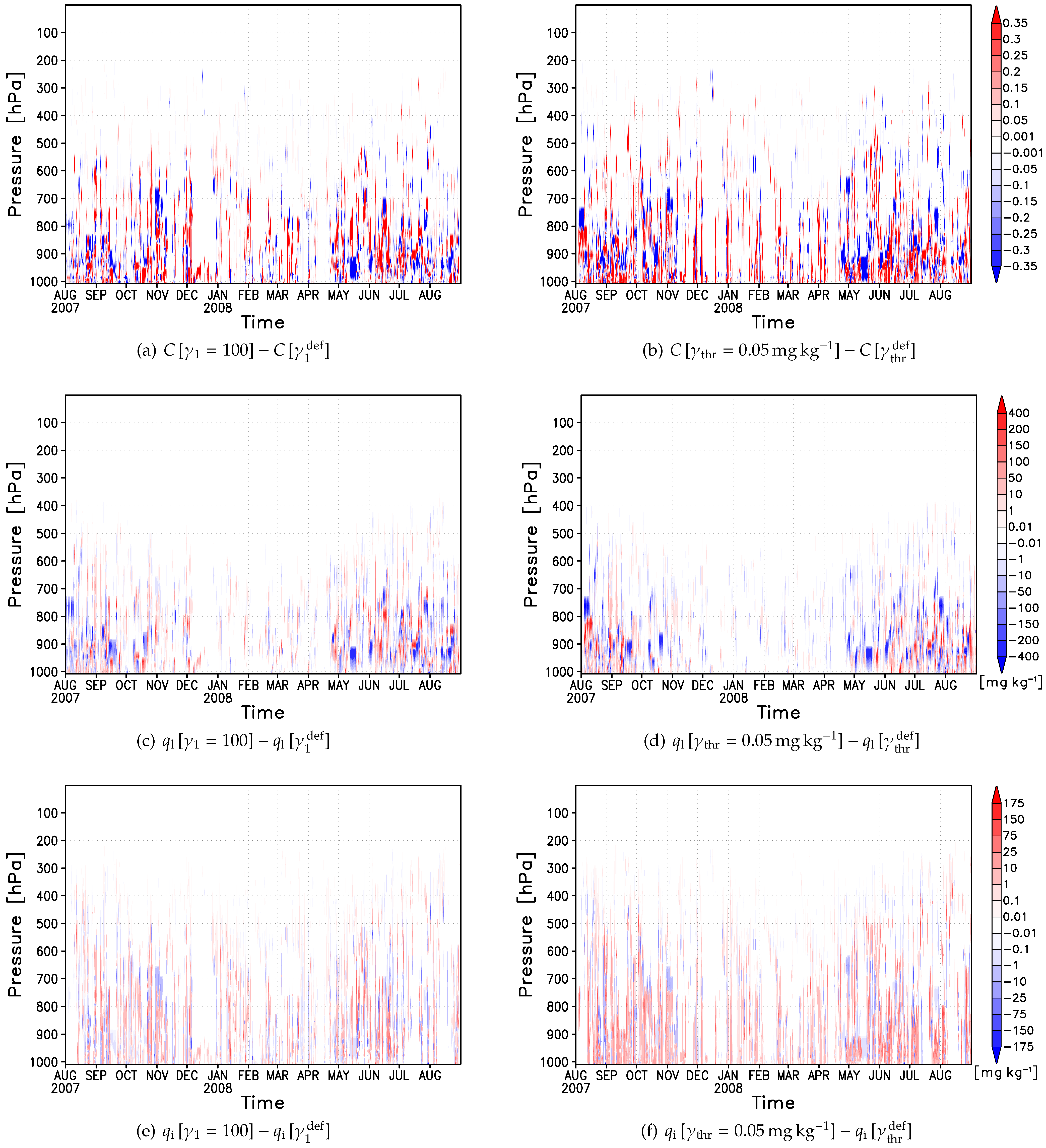
Figure 5. Difference plots (SENS minus CTRL) of simulated fractional cloud cover (top), cloud water content (middle), and cloud ice content (bottom) for one lower value of the PS-Scheme adjustment parameter (left column) and one higher value of the tunable parameter (right column), with and . These sensitivity experiments were conducted at the NP-35 start position simulating from 1 August 2007 to 31 August 2008 by analogy to the reference run (Figure 3).

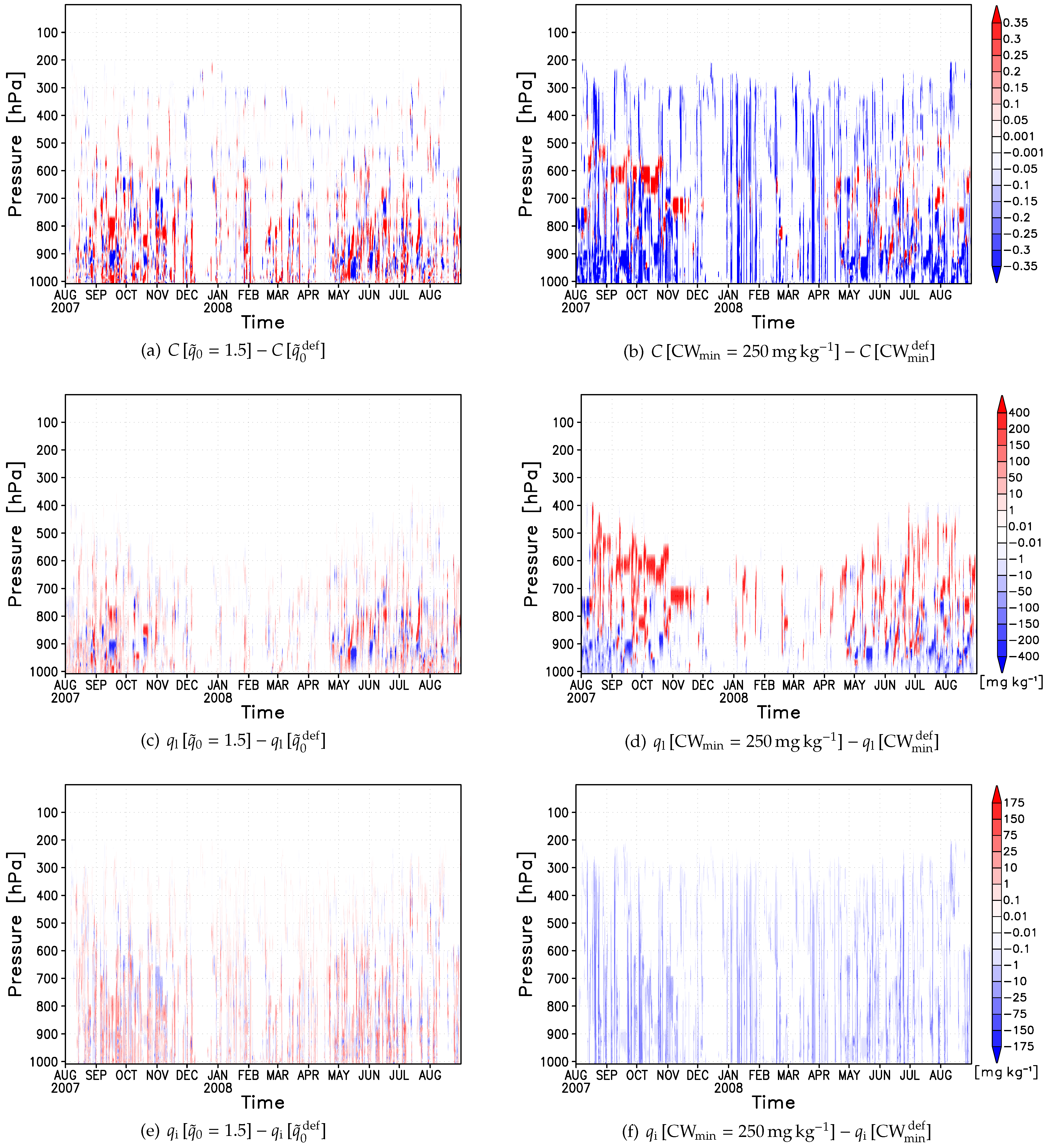The third column of Table 4 and Table 5 reveal that overall a lower (higher) value of leads to a reduction of (rise in) . Indeed mid- and high-level clouds decrease significantly due to lower parameter values while low-level clouds tend to slightly increase (see Figure 5(a)). One possible reason for the increase at lower levels might be very low saturation water contents due to cold temperatures in the relatively wet boundary layer over the Arctic Ocean favoring cloud formation. Although lower values of are able to reduce and rise (overall increase in suggested by Figure 5(c)) as well as , the overestimation of is strengthened (overall increase in suggested by Figure 5(e)). Both and rise amplifying the overestimation of as well.

The second adjustment parameter K, which relates the increase in the skewness parameter to the detrainment of cloud condensate, was varied in the co-domain . However, modifying this parameter only leads to temporary local changes of C (not shown), and overall remains almost unaffected. This can be attributed to the minor role of convection in cloud formation over the ice-covered Arctic Ocean, unless open water areas in terms of polynyas or leads coexist. Other cloud-related model variables either remain almost unchanged or increase in part significantly by changes in K. Both the overestimation of ( ) and is strengthened. Furthermore, only higher parameter values of K enable convective precipitation during wintertime (WP) explaining the increase of 100% in the fourth column of Table 5.

4.2. Modified Tuning Parameters of Cloud Microphysics

The following discussions will basically concentrate on tuning parameters of the cloud microphysics, which can reduce based on Table 4 and Table 5, and conclusions are summarized in Table 6.

Table 6. Overall effect on cloud-related model variables due to modification of a single model tuning parameter enabling the reduction of relative to the default parameter value (see Table 1 and Figure 4). Effects that potentially improve model results are marked by a ‘+’, negative influences are indicated by a ‘−’.

Parameter	Changes due to lower parameter value	Changes due to higher parameter value
	1.5	20
	reduction of and	rise in ( ) but reduction of ( );
	rise in ( )	effect is small (large) for ( )
	rise in ( )	rise in , , , and
	rise in and
	rise in ( ) but reduction of ( );	significant reduction of ,
	effect is more pronounced than for higher	reduction of
	and more significant for	reduction of ( ) but rise in ( )
	rise in , , , and	and
	5	100
	( ) rises but reduction of	rise in ( ) but reduction of ( );
	rise in all other regarded model variables	effect is large (small) for ( )
		significant decrease in ,
		rise in and
	rise in ( ) but reduction of ( ),	( ) rises
	where effect is significant for and	rise in all remaining model variables
	reduction of ,
	increase in and

Table 6. Overall effect on cloud-related model variables due to modification of a single model tuning parameter enabling the reduction of relative to the default parameter value (see Table 1 and Figure 4). Effects that potentially improve model results are marked by a ‘+’, negative influences are indicated by a ‘−’.

Parameter	Changes due to lower parameter value	Changes due to higher parameter value
	1.5	20
	reduction of and	rise in ( ) but reduction of ( );
	rise in ( )	effect is small (large) for ( )
	rise in ( )	rise in , , , and
	rise in and
	rise in ( ) but reduction of ( );	significant reduction of ,
	effect is more pronounced than for higher	reduction of
	and more significant for	reduction of ( ) but rise in ( )
	rise in , , , and	and
	5	100
	( ) rises but reduction of	rise in ( ) but reduction of ( );
	rise in all other regarded model variables	effect is large (small) for ( )
		significant decrease in ,
		rise in and
	rise in ( ) but reduction of ( ),	( ) rises
	where effect is significant for and	rise in all remaining model variables
	reduction of ,
	increase in and

To assess the impact of modified , sensitivity experiments were conducted in the wide range between zero and . Note that impacts model results by ensuring nonzero and regardless of the applied cloud scheme (see Table 1). As a working hypothesis, lower (higher) should result in rising (declining) cloud cover. This is generally confirmed by the fifth column of Table 4 and Table 5. Higher lead to significant decrease in , and very high parameter values are even able to prevent the formation of clouds. While low- and high-level clouds tend to decline monotonically, mid-level clouds first seem to increase but finally decrease as well (suggested by Figure 5(b)). Despite the ability to reduce the overestimation of , higher amplify the over- and underestimation of and , respectively. During the entire simulation period decreases below 900h but significantly increases above 900h, while decreases monotonically (see Figure 5(d,f)). Furthermore, higher amplify the overestimation of while and drop.

The autoconversion rate , which controls the conversion from (supercooled) cloud droplets to rain drops and thus the cloud lifetime effect, was found to be the next promising tuning parameter. This parameter was varied in the co-domain . Figure 6(a) and the sixth column of Table 4 and Table 5 confirm that only higher parameter values might be able to improve simulated cloudiness. Here, the increase in during wintertime (WP) is outweighed by the decrease during summertime (SP). Furthermore, higher are able to reduce the over- and underestimation of and , respectively. For and this effect is more difficult to identify from Figure 6(c,e) due to temporary local changes. As expected, and rise in case of higher amplifying the overestimation of , while is more or less unaffected.

Finally, the cloud ice threshold was identified as promising tuning parameter. This parameter controls the Bergeron–Findeisen process, which explains the growth of ice crystals at the expense of cloud droplets in mixed-phase clouds due to lower vapor pressures over ice than over water at subfreezing temperatures. Lohman et al. [66] have pointed out that as soon as the threshold of cloud ice content is exceeded a supercooled water cloud will glaciate immediately in the model. In the standard ECHAM5 code the remaining cloud water is not evaporated to deposit onto existing ice crystals but remaining cloud droplets have to either freeze or grow to precipitable sizes in subsequent time steps. For the sake of completeness was varied from zero to . As shown by Figure 6(b) and the last column of Table 4 and Table 5, lower are also able to reduce the overestimation of simulated Arctic clouds. Furthermore, a lower parameter value is most suitable to improve the modeled ratio of to (overall reduction of but rise in , see Figure 6(d,f)), which can be associated with the most significant reduction of but rise in . While decreases and remains almost unchanged, increases overall.

Figure 6. Difference plots (SENS minus CTRL) of simulated fractional cloud cover (top), cloud water content (middle), and cloud ice content (bottom) for one higher value of the tunable parameter (left column) and one lower value of the tunable parameter (right column), with and . These sensitivity experiments were conducted at the NP-35 start position simulating from 1 August 2007 to 31 August 2008 by analogy to the reference run (Figure 3).

Figure 6. Difference plots (SENS minus CTRL) of simulated fractional cloud cover (top), cloud water content (middle), and cloud ice content (bottom) for one higher value of the tunable parameter (left column) and one lower value of the tunable parameter (right column), with and . These sensitivity experiments were conducted at the NP-35 start position simulating from 1 August 2007 to 31 August 2008 by analogy to the reference run (Figure 3).

Figure 7 shows the comparison of monthly averaged by analogy to Section 3.2.2. Here, only the annual cycles of the best-fit parameters (green curves), based on the best combination of lowest 13-month-mean of and overall RMSE, are shown in addition to the annual cycle produced by MODIS (black curve) and using the default values (blue curve), respectively. Note that MODIS and the HIRHAM5-SCM reference run (using the PS-Scheme) produced averaged of 64.8% and 78.2%, respectively with an overall RMSE of 18.4% (see Table 3). Thus, Figure 7 confirms that higher (averaged of 77.3% and overall RMSE of 17.2% for ) and (averaged of 77.8% and overall RMSE of 17.3% for ) as well as lower (averaged of 76.5% and overall RMSE of 17.9% for ) and (averaged of 74.9% and overall RMSE of 14.1% for ) reduce simulated Arctic cloud cover, where the latter might be the most promising tuning parameter to improve cloud-related variables in the model.

Figure 7. Monthly means of (in %) from August 2007 to August 2008 referring to the NP-35 start position. The results originate from MODIS (black line) satellite observations, and HIRHAM5-SCM simulations using either the PS-Scheme and default model parameters (blue line) or the PS-Scheme with a single modified tuning parameter (green lines).

Figure 7. Monthly means of (in %) from August 2007 to August 2008 referring to the NP-35 start position. The results originate from MODIS (black line) satellite observations, and HIRHAM5-SCM simulations using either the PS-Scheme and default model parameters (blue line) or the PS-Scheme with a single modified tuning parameter (green lines).

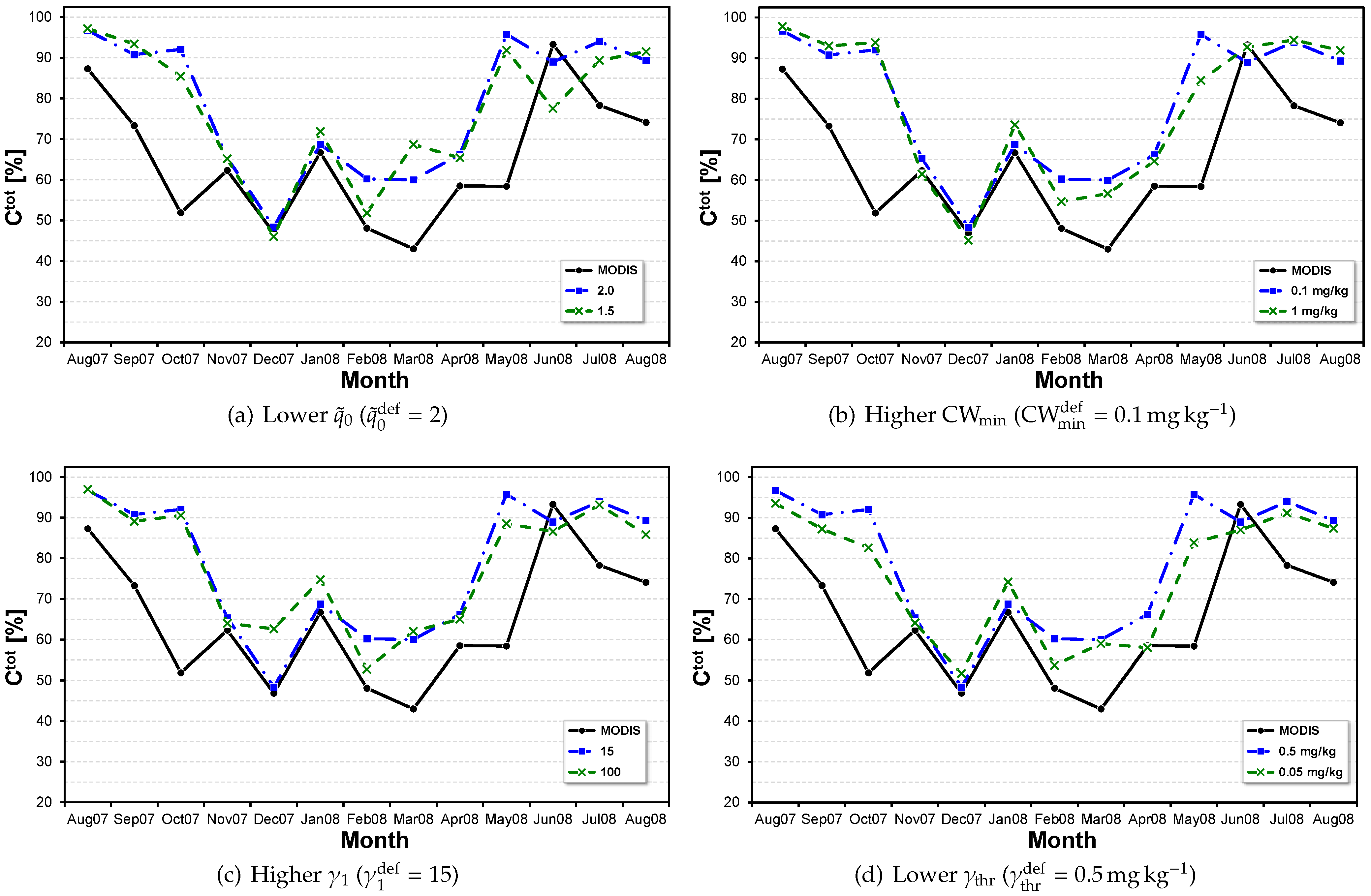Figure 7 also reveals that all four tuning parameters are able to reduce during May 2008 while only modified and improve the simulation of Arctic clouds during October 2007. In the former case, the enhanced cloud formation due to unrealistic turbulent moisture fluxes could be either partially compensated due to more efficient precipitation processes (for and ) or through the partial suppression of cloud formation (for and ). In the latter case, both the more deficient simulation of the ABL structure and the overestimated cloud top radiative cooling could not be significantly improved by changing tuning parameters of the cloud microphysics, except for . The most significant impact through reduced in both cases can be explained with the more efficient Bergeron–Findeisen process which results in faster growing cloud ice particles and finally enhanced snow fall.

5. Conclusions

A SCM version of the atmospheric RCM HIRHAM5 was developed to analyze the representation of Arctic clouds. HIRHAM5-SCM was exploited as test bed for evaluating the cloud cover schemes of the ECHAM5 parameterization package, the RH-Scheme by Sundquist et al. [52] and the more sophisticated PS-Scheme by Tompkins [45].

Observations from the 35th Russian North Pole drifting station (NP-35) were used to validate the model. Above the Arctic boundary layer (ABL), simulated and observed temperature profiles agree fairly well. In contrast, the more pronounced vertical variability of relative humidity is inadequately reproduced. Primarily the RH-Scheme produces clouds at incorrect altitudes. The PS-Scheme enables to better simulate the observed correlation between the occurrence of boundary layer clouds (BLCs) and capping strong temperature inversion as well as rapid moisture decrease. Further, the PS-Scheme results in higher correlations between the simulated and the measured temperature and humidity profiles. Nevertheless, the model has difficulties in simulating the ABL, most likely due to unrealistic turbulent exchange under extremely stable conditions.

The evaluation of relative frequencies of simulated clear-sky, partially cloudy, and (totally) overcast cases revealed underestimation of clear-sky and overestimation of overcast conditions as compared to ground-based observations at NP-35. Both biases are significantly larger when using the RH-Scheme, even though the frequency of partially cloudy conditions agrees well. Overall, the overestimation of cloudy cases (sum of partially cloudy and overcast cases) is reduced by the PS-Scheme.

Independent from the used cloud scheme, the higher frequency of occurrence of modeled low-level clouds during summer (JJA) and autumn (SON) is in accordance with the frequently observed presence of summertime BLCs [13,14]. However, the PS-Scheme simulates cloud formation and dissipation more realistically, since the cloud cover is directly linked to sources and sinks (like turbulence, convection, and microphysics), enabling the simulation of frequently observed abrupt changes between overcast and clear-sky conditions.

The validation of the simulated annual cycle of total cloud cover against ISCCP-D2 and MODIS satellite observations showed qualitative agreement with MODIS in terms of higher cloud cover in summer and lower cloud cover in winter. The annual cycle of ISCCP-D2 is reversed and might be unrealistic as has already been pointed out by Schweiger et al. [71] and as is suggested by comparison with the ground-based observations at NP-35.

The qualitative agreement with MODIS is independent from the cloud cover scheme, but the RH-Scheme systematically overestimates the cloud cover, while the PS-Scheme shows reduced biases and pretty good agreement from November to January. However, the transition from high cloud cover in summer to lower cloud cover in winter and vice versa is shifted to the cold season in either case, accompanied by large biases in October and May.

All in all, the PS-Scheme enables an improved simulation of Arctic clouds as compared to the RH-Scheme, but it still shows a systematic overestimation of Arctic cloud cover. Several tunable parameters were analyzed by means of sensitivity studies to identify parameters which potentially enable the adaptation of the cloud parameterization to Arctic climate conditions. The resulting recommendations are summarized below:

• • Lower values of , the parameter that determines the shape of the symmetric beta distribution in the PS-Scheme, result in a reduction of total cloud cover ( best fit to MODIS), decreased underestimation of cloud ice, but increased overestimation of cloud water and precipitation.
• • Higher values of the minimum cloud water content result in a reduction of clouds (even up to their total disappearance) and consequently decreased overestimation of total cloud cover ( best fit to MODIS), but also in increased overestimation/underestimation of cloud water/cloud ice and increased overestimation of precipitation. Instead of applying the same value of to cloud water and cloud ice, it is suggested using different thresholds, since cloud water contents are typically about one magnitude higher than cloud ice contents in Arctic clouds (e.g., [28,47]).
• • Higher values of the autoconversion rate , which controls the local rain production and thus the cloud lifetime, result in decreased overestimation of total cloud cover ( best fit to MODIS), decreased overestimation/underestimation of cloud water/cloud ice, but increased overestimation of precipitation as was expected.
• • Lower values of the cloud ice threshold , which controls the efficiency of the Bergeron–Findeisen process, turned out to be most suitable for reducing the overestimation of total cloud cover ( best fit to MODIS) and result additionally in decreased overestimation/underestimation of cloud water/cloud ice, but also increased overestimation of precipitation.

The best-fit parameters suggested by this study need to be examined for their performance in the three-dimensional model version HIRHAM5. Liu et al. [77] have identified the possible underestimation of MODIS relative to CloudSat-CALIPSO cloud amount especially over the ice-covered Arctic ocean. It is therefore planned to validate cloud-related variables simulated by HIRHAM5 against observations from the Multiangle Imaging SpectroRadiometer (MISR) and Cloud Aerosol Lidar with Orthogonal Polarization (CALIOP). Since changes in modeled cloud fraction and total precipitation are anti-correlated, extensive validation against precipitation observations is required. This is currently ongoing work.

References

- Schneider, S.H. Cloudiness as a global climate feedback mechanism: The effects on the radiation balance and surface temperature of variations in cloudiness. J. Atmos. Sci. 1972, 29, 1413–1422. [Google Scholar] [CrossRef]
- Minnett, P.J. The influence of solar zenith angle and cloud type on cloud radiative forcing at the surface in the Arctic. J. Clim. 1999, 12, 147–158. [Google Scholar] [CrossRef]
- Shupe, M.D.; Intrieri, J.M. Cloud radiative forcing of the Arctic surface: The influence of cloud properties, surface albedo, and solar zenith angle. J. Clim. 2004, 17, 616–628. [Google Scholar] [CrossRef]
- Hu, R.M.; Blanchet, J.P.; Girard, E. The effect of aerosol on surface cloud radiative forcing in the Arctic. Atmos. Chem. Phys. Discuss. 2005, 5. [Google Scholar] [CrossRef]
- Gorodetskaya, I.V.; Tremblay, L.B.; Liepert, B.; Cane, M.A.; Cullather, R.I. The influence of cloud and surface properties on the Arctic ocean shortwave radiation budget in coupled models. J. Clim. 2008, 21. [Google Scholar] [CrossRef]
- Lee, S.S.; Donner, L.J.; Phillips, V.T.J. Sensitivity of aerosol and cloud effects on radiation to cloud types: Comparison between deep convective clouds and warm stratiform clouds over one-day period. Atmos. Chem. Phys. 2009, 9. [Google Scholar] [CrossRef]
- Ramanathan, V.; Cess, R.D.; Harrison, E.F.; Minnis, P.; Barkstrom, B.R.; Ahmad, E.; Hartmann, D. Cloud-radiative forcing and climate: Results from the earth radiation budget experiment. Science 1989, 243, 57–63. [Google Scholar]
- Walsh, J.E.; Chapman, W.L. Arctic cloud-radiation-temperature associations in observational data and atmospheric reanalyses. J. Clim. 1998, 11, 3030–3045. [Google Scholar] [CrossRef]
- Intrieri, J.M.; Fairall, C.W.; Shupe, M.D.; Persson, P.O.G.; Andreas, E.L.; Guest, P.S.; Moritz, R.E. An annual cycle of Arctic surface cloud forcing at SHEBA. J. Geophys. Res. 2002, 107. [Google Scholar] [CrossRef]
- Kahl, J.D.; Martinez, D.A.; Zaitseva, N.A. Long-term variability in the low-level inversion layer over the Arctic ocean. Int. J. Climatol. 1996, 16, 1297–1313. [Google Scholar] [CrossRef]
- Zhang, Y.; Seidel, D.J.; Golaz, J.C.; Deser, C.; Tomas, R.A. Climatological characteristics of Arctic and Antarctic surface-based inversions. J. Clim. 2011, 24. [Google Scholar] [CrossRef]
- Mauritsen, T.; Sedlar, J.; Tjernström, M.; Leck, C.; Martin, M.; Shupe, M.; Sjogren, S.; Sierau, B.; Persson, P.O.G.; Brooks, I.M.; et al. An Arctic CCN-limited cloud-aerosol regime. Atmos. Chem. Phys. 2011, 11. [Google Scholar] [CrossRef] [Green Version]
- Herman, G.; Goody, R. Formation and persistence of summertime Arctic stratus clouds. J. Atmos. Sci. 1976, 33, 1537–1553. [Google Scholar] [CrossRef]
- Curry, J.A.; Rossow, W.B.; Randall, D.; Schramm, J.L. Overview of Arctic cloud and radiative characteristics. J. Clim. 1996, 9, 1731–1764. [Google Scholar] [CrossRef]
- Intrieri, J.M.; Shupe, M.D.; Uttal, T.; McCarty, B.J. An annual cycle of Arctic cloud characteristics observed by radar and lidar at SHEBA. J. Geophys. Res. 2002, 107. [Google Scholar] [CrossRef]
- Kay, J.E.; Gettelman, A. Cloud influence on and response to seasonal Arctic sea ice loss. J. Geophys. Res. 2009, 114. [Google Scholar] [CrossRef]
- Eastman, R.; Warren, S.G. Interannual variations of Arctic cloud types in relation to sea ice. J. Clim. 2010, 23. [Google Scholar] [CrossRef]
- Eastman, R.; Warren, S.G. Arctic cloud changes from surface and satellite observations. J. Clim. 2010, 23. [Google Scholar] [CrossRef]
- Walsh, J.E.; Kattsov, V.M.; Chapman, W.L.; Govorkova, V.; Pavlova, T. Comparison of Arctic climate simulations by uncoupled and coupled global models. J. Clim. 2002, 15, 1429–1446. [Google Scholar] [CrossRef]
- Inoue, J.; Liu, J.; Pinto, J.O.; Curry, J.A. Intercomparison of Arctic regional models: Modeling clouds and radiation for SHEBA in May 1998. J. Clim. 2006, 19. [Google Scholar] [CrossRef]
- Tjernström, M.; Sedlar, J.; Shupe, M.D. How well do regional climate models reproduce radiation and clouds in the Arctic? An evaluation of ARCMIP simulations. J. Appl. Meteorol. Climatol. 2008, 47. [Google Scholar] [CrossRef]
- Birch, C.E.; Brooks, I.M.; Tjernström, M.; Milton, S.F.; Earnshaw, P.; Soderberg, S.; Persson, P.O.G. The performance of a global and mesoscale model over the central Arctic ocean during late summer. J. Geophys. Res. 2009, 114. [Google Scholar] [CrossRef]
- Arking, A. The radiative effects of clouds and their impact on climate. Bull. Am. Meteorol. Soc. 1991, 71, 795–813. [Google Scholar] [CrossRef]
- Cess, R.D.; Zhang, M.H.; Ingram, W.J.; Potter, G.L.; Alekseev, V.; Barker, H.W.; Cohen-Solal, E.; Colman, R.A.; Dazlich, D.A.; Del Genio, A.D.; et al. Cloud feedback in atmospheric general circulation models: An update. J. Geophys. Res. 1996, 101. [Google Scholar] [CrossRef]
- Solomon, S.; Qin, D.; Manning, M.; Chen, Z.; Marquis, M.; Averyt, K.B.; Tignor, M.; Miller, H.L. Climate Change 2007: The Physical Science Basis : Contribution of Working Group I to the Fourth Assessment Report of the Intergovernmental Panel on Climate Change; Cambridge University Press: Cambridge, UK, 2007; pp. 629–640. [Google Scholar]
- Curry, J.A.; Pinto, J.O.; McInnes, K.L. Modeling the Summertime Arctic Cloudy Boundary Layer. In Proceedings of the Fifth Atmospheric Radiation Measurement (ARM) Science Team Meeting; Department of Energy/Atmospheric Radiation Measurement (DOE/ARM), San Diego, CA, USA, 19–23 March 1995; pp. 63–67.
- Morrison, H.; Pinto, J.O. Intercomparison of bulk cloud microphysics schemes in mesoscale simulations of springtime Arctic mixed-phase stratiform clouds. Mon. Weather Rev. 2006, 134, 1880–1900. [Google Scholar] [CrossRef]
- Sednev, I.; Menon, S.; McFarquhar, G. Simulating mixed-phase Arctic stratus clouds: Sensitivity to ice initiation mechanisms. Atmos. Chem. Phys. 2009, 9. [Google Scholar] [CrossRef]
- Inoue, J.; Kosovic, B.; Curry, J.A. Evolution of a storm-driven cloudy boundary layer in the Arctic. Bound. Layer Meteorol. 2005, 117. [Google Scholar] [CrossRef]
- Wyser, K.; Jones, C.G.; Du, P.; Girard, E.; Willén, U.; Cassano, J.; Christensen, J.H.; Curry, J.A.; Dethloff, K.; Haugen, J.E.; et al. An evaluation of Arctic cloud and radiation processes during the SHEBA year: Simulation results from eight Arctic regional climate models. Clim. Dyn. 2008, 30. [Google Scholar] [CrossRef]
- Luo, Y.; Xu, K.M.; Morrison, H.; McFarquhar, G. Arctic mixed-phase clouds simulated by a cloud-resolving model: Comparison with ARM observations and sensitivity to microphysics parameterizations. J. Atmos. Sci. 2008, 65. [Google Scholar] [CrossRef]
- Klein, S.A.; McCoy, R.B.; Morrison, H.; Ackerman, A.S.; Avramov, A.; de Boer, G.; Chen, M.; Cole, J.N.S.; Del Genio, A.D.; Falk, M.; et al. Intercomparison of model simulations of mixed-phase clouds observed during the ARM mixed-phase Arctic cloud experiment. I: Single-layer cloud. Q. J. R. Meteorol. Soc. 2009, 135. [Google Scholar] [CrossRef]
- Lubin, D.; Vogelmann, A.M. A climatologically significant aerosol longwave indirect effect in the Arctic. Nature 2006, 439, 453–456. [Google Scholar]
- Garrett, T.J.; Zhao, C. Increased Arctic cloud longwave emmisivity associated with pollution from mid-latitudes. Nature 2006, 440, 787–789. [Google Scholar] [CrossRef]
- Morrison, H.; Pinto, J.O.; Curry, J.A.; McFarquhar, G.M. Sensitivity of modeled Arctic mixed-phase stratocumulus to cloud condensation and ice nuclei over regionally varying surface conditions. J. Geophys. Res. 2008, 113. [Google Scholar] [CrossRef]
- Morrison, H.; McCoy, R.B.; Klein, S.A.; Xie, S.; Luo, Y.; Avramov, A.; Chen, M.; Cole, J.N.S.; Falk, M.; Foster, M.J.; et al. Intercomparison of model simulations of mixed-phase clouds observed during the ARM mixed-phase Arctic cloud experiment. II: Multilayer cloud. Q. J. R. Meteorol. Soc. 2009, 135. [Google Scholar] [CrossRef]
- Hannay, C.; Bhatt, U.S.; Harrington, J.Y. Single-Column Model Simulations of Arctic Cloudiness and Surface Radiative Fluxes during the Surface Heat Budget of the Arctic (SHEBA) Experiment. In Proceedings of the 6th Conference on Polar Meteorology and Oceanography; American Meteorological Society (AMS), San Diego, CA, USA,, 14–18 May 2001.
- Kay, J.E.; Raeder, K.; Gettelman, A.; Anderson, J. The boundary layer response to recent Arctic sea ice loss and implications for high-latitude climate feedbacks. J. Clim. 2011, 24. [Google Scholar] [CrossRef]
- Pinto, J.O.; Curry, J.A. Atmospheric convective plumes emanating from leads 2. Microphysical and radiative processes. J. Geophys. Res. 1995, 100, 4633–4642. [Google Scholar]
- Curry, J.A.; Hobbs, P.V.; King, M.D.; Randall, D.A.; Minnis, P.; Isaac, G.A.; Pinto, J.O.; Uttal, T.; Bucholtz, A.; Cripe, D.G.; et al. FIRE Arctic clouds experiment. Bull. Am. Meteorol. Soc. 2000, 81, 5–29. [Google Scholar] [CrossRef]
- Rozwadowska, A.; Cahalan, R.F. Plane-parallel biases computed from inhomogeneous Arctic clouds and sea ice. J. Geophys. Res. 2002, 107. [Google Scholar] [CrossRef]
- Sato, K.; Inoue, J.; Kodama, Y.M.; Overland, J.E. Impact of Arctic sea-ice retreat on the recent change in cloud-base height during autumn. Geophys. Res. Lett. 2012, 39. [Google Scholar] [CrossRef]
- Lohmann, U.; Roeckner, E. Design and performance of a new cloud microphysics parametrization developed for the ECHAM general circulation model. Clim. Dyn. 1996, 12, 557–572. [Google Scholar] [CrossRef]
- Salzmann, M.; Ming, Y.; Golaz, J.C.; Ginoux, P.A.; Morrison, H.; Gettelman, A.; Krämer, M.; Donner, L.J. Two-moment bulk stratiform cloud microphysics in the GFDL AM3 GCM: Description, evaluation, and sensitivity tests. Atmos. Chem. Phys. 2010, 10. [Google Scholar] [CrossRef]
- Tompkins, A.M. A prognostic parameterization for the subgrid-scale variability of water vapor and clouds in large-scale models and its use to diagnose cloud cover. J. Atmos. Sci. 2002, 59, 1917–1942. [Google Scholar] [CrossRef]
- Zhu, P.; Zuidema, P. On the use of PDF schemes to parameterize sub-grid clouds. Geophys. Res. Lett. 2009, 36. [Google Scholar] [CrossRef]
- Pinto, J.O.; Curry, J.A.; Lynch, A.H.; Persson, P.O.G. Modeling clouds and radiation for the November 1997 period of SHEBA using a column climate model. J. Geophys. Res. 1999, 104. [Google Scholar] [CrossRef]
- Dethloff, K.; Abegg, C.; Rinke, A.; Hebestadt, I.; Romanov, V.F. Sensitivity of Arctic climate simulations to different boundary layer parameterizations in a regional climate model. Tellus A 2001, 53, 1–26. [Google Scholar]
- Zhang, J.; Lohmann, U. Sensitivity of single column model simulations of Arctic springtime clouds to different cloud cover and mixed phase cloud parameterizations. J. Geophys. Res. 2003, 108. [Google Scholar] [CrossRef]
- Morrison, H.; Curry, J.A.; Shupe, M.D.; Zuidema, P. A new double-moment microphysics parameterization for application in cloud and climate models. part II: Single-column modeling of Arctic clouds. J. Atmos. Sci. 2005, 62. [Google Scholar] [CrossRef]
- The HIRHAM Regional Climate Model Version 5(β); Technical Report 06-17; Danish Meteorological Institute (DMI): Copenhagen, Denmark, 2007.
- Sundquist, H.; Berge, E.; Kristjánsson, J.E. Condensation and cloud parameterization studies with a mesoscale numerical weather prediction model. Mon. Weather Rev. 1989, 117, 1641–1657. [Google Scholar] [CrossRef]
- Undén, P.; Rontu, L.; Järvinen, H.; Lynch, P.; Calvo, J.; Cats, G.; Cuxart, J.; Eerola, K.; Fortelius, C.; Garcia-Moya, J.A.; et al. HIRLAM-5 Scientific Documentation. In HIRLAM-5 Project; Swedish Meteorological and Hydrological Institute (SMHI): Norrköping, Sweden, 2002. [Google Scholar]
- The Atmospheric General Circulation Model ECHAM5–Part I: Model Description; Technical Report 349; Max Planck Institute (MPI) for Meteorology: Hamburg, Germany, 2003.
- The ERA–Interim Archive; ERA report series; European Center for Medium-Range Weather Forecasts (ECMWF): Reading, UK, 2009.
- Bergman, J.W.; Sardeshmukh, P.D. Dynamic stabilization of atmospheric single column models. J. Clim. 2004, 17, 1004–1021. [Google Scholar] [CrossRef]
- Dee, D.P.; Uppala, S.M.; Simmons, A.J.; Berrisford, P.; Poli, P.; Kobayashi, S.; Andrae, U.; Balmaseda, M.A.; Balsamo, G.; Bauer, P.; et al. The ERA-Interim reanalysis: Configuration and performance of the data assimilation system. Q. J. R. Meteorol. Soc. 2011, 137, 553–597. [Google Scholar] [CrossRef]
- Randall, D.A.; Cripe, D.G. Alternative methods for specification of observed forcing in single-column models and cloud system models. J. Geophys. Res. 1999, 104. [Google Scholar] [CrossRef]
- Lohmann, U.; McFarlane, N.; Levkov, L.; Abdella, K.; Albers, F. Comparing different cloud schemes of a single column model by using mesoscale forcing and nudging technique. J. Clim. 1999, 12, 438–461. [Google Scholar] [CrossRef]
- Atmospheric Investigations on the Russian North Pole Drifting Ice Station NP-35. Available online: http://www.awi.de/en/research/research_divisions/climate_science/atmospheric_circulations/expeditions_campaigns/np_35/ (accessed on 9 August 2012).
- The Atmospheric General Circulation Model ECHAM4: Model Description and Simulation of Present-Day Climate; Technical Report 218; Max Planck Institute (MPI) for Meteorology: Hamburg, Germany, 1996.
- Wild, M.; Roeckner, E. Radiative fluxes in the ECHAM5 general circulation model. J. Clim. 2006, 19. [Google Scholar] [CrossRef]
- Tiedtke, M. A comprehensive mass flux scheme for cumulus parameterization in large-scale models. Mon. Weather Rev. 1989, 117, 1179–1800. [Google Scholar]
- Nordeng, T.E. Extended Versions of the Convective Parametrization Scheme at ECMWF and Their Impact on the Mean and Transient Activity of the Model in the Tropics. In Technical Memorandum; European Center for Medium-Range Weather Forecasts (ECMWF): Reading, UK, 1994. [Google Scholar]
- Wang, S.; Wang, Q.; Jordan, R.E.; Persson, P.O.G. Interactions among longwave radiation of clouds, turbulence, and snow surface temperature in the Arctic: A model sensitivity study. J. Geophys. Res. 2001, 106. [Google Scholar] [CrossRef]
- Lohmann, U.; Stier, P.; Hoose, C.; Ferrachat, S.; Kloster, S.; Roeckner, E.; Zhang, J. Cloud microphysics and aerosol indirect effects in the global climate model ECHAM5-HAM. Atmos. Chem. Phys. 2007, 7, 3425–3446. [Google Scholar] [CrossRef]
- Rossow, W.B.; Schiffer, R.A. Advances in understanding clouds from ISCCP. Bull. Am. Meteorol. Soc. 1999, 80, 2261–2287. [Google Scholar] [CrossRef]
- International Satellite Cloud Climatology Project (ISCCP) by NASA Goddard Institute for Space Studies (GISS). Available online: ftp://isccp.giss.nasa.gov/pub/data/D2Tars/ (accessed on 25 August 2011).
- MODIS Atmosphere L3 Gridded Product Algorithm Theoretical Basis Document. Available online: http://modis-atmos.gsfc.nasa.gov/_docs/MOD08MYD08%20ATBD%20C005.pdf (accessed on 9 August 2012).
- Moderate Resolution Imaging Spectroradiometer (MODIS) by National Aeronautics and Space Administration (NASA). Available online: ftp://ladsweb.nascom.nasa.gov/allData/5/MOD08_M3/ (accessed on 14 October 2011).
- Schweiger, A.J.; Lindsay, R.W.; Key, J.R.; Francis, J.A. Arctic clouds in multilayer satellite data sets. Geophys. Res. Lett. 1999, 26, 1845–1848. [Google Scholar] [CrossRef]
- Hahn, C.J.; Warren, S.G.; London, J. The effect of moonlight on observations of cloud cover at night, and application to cloud climatology. J. Clim. 1995, 8, 1429–1466. [Google Scholar] [CrossRef]
- Wielicki, B.A.; Parker, L. On the determination of cloud cover from satellite sensors: The effect of sensor spatial resolution. J. Geophys. Res. 1992, 97. [Google Scholar] [CrossRef]
- Zhao, M.; Wang, Z. Comparison of Arctic clouds between European Center for Medium-Range Weather Forecasts simulations and Atmospheric Radiation Measurement Climate Research Facility long-term observations at the North Slope of Alaska Barrow Site. J. Geophys. Res. 2010, 115. [Google Scholar] [CrossRef]
- Axelsson, P.; Tjernström, M.; Söderberg, S.; Svensson, G. An ensemble of Arctic simulations of the AOE-2001 field experiment. Atmosphere 2011, 2. [Google Scholar] [CrossRef]
- Weber, T.; Quaas, J.; Räisänen, P. Evaluation of the statistical cloud scheme in the ECHAM5 model using satellite data. Q. J. R. Meteorol. Soc. 2011, 137. [Google Scholar] [CrossRef]
- Liu, Y.; Ackerman, S.A.; Maddux, B.C.; Key, J.R.; Frey, R.A. Errors in cloud detection over the Arctic using a satellite imager and implications for observing feedback mechanisms. J. Clim. 2010, 23. [Google Scholar] [CrossRef]
© 2012 by the authors; licensee MDPI, Basel, Switzerland. This article is an open-access article distributed under the terms and conditions of the Creative Commons Attribution license (http://creativecommons.org/licenses/by/3.0/).
Share and Cite
Klaus, D.; Dorn, W.; Dethloff, K.; Rinke, A.; Mielke, M. Evaluation of Two Cloud Parameterizations and Their Possible Adaptation to Arctic Climate Conditions. Atmosphere 2012, 3, 419-450. https://doi.org/10.3390/atmos3030419
Klaus D, Dorn W, Dethloff K, Rinke A, Mielke M. Evaluation of Two Cloud Parameterizations and Their Possible Adaptation to Arctic Climate Conditions. Atmosphere. 2012; 3(3):419-450. https://doi.org/10.3390/atmos3030419
Chicago/Turabian StyleKlaus, Daniel, Wolfgang Dorn, Klaus Dethloff, Annette Rinke, and Moritz Mielke. 2012. "Evaluation of Two Cloud Parameterizations and Their Possible Adaptation to Arctic Climate Conditions" Atmosphere 3, no. 3: 419-450. https://doi.org/10.3390/atmos3030419
APA StyleKlaus, D., Dorn, W., Dethloff, K., Rinke, A., & Mielke, M. (2012). Evaluation of Two Cloud Parameterizations and Their Possible Adaptation to Arctic Climate Conditions. Atmosphere, 3(3), 419-450. https://doi.org/10.3390/atmos3030419