1. Introduction
Determining spatial and temporal variability of atmospheric variables is an essential aspect of climate studies, particularly those focusing on climate variability and change. The occurrence of extreme events in weather and climate variables pose major threats to human and natural systems. It is essential to understand aspects such as recurrence of severe events, magnitude, and duration. The longer the timeseries available the better. However, the handling of such extended timeseries results in a number of statistical challenges, particularly when both linear and nonlinear relationships determine the evolution of the variable under consideration. While variables such as temperature, pressure, or winds are fields with few occasional local, temporal discontinuities and/or sharp gradients, this is not the case with precipitation. Precipitation and its source, clouds, are highly localized phenomena, both in space and in time. Its occurrence and form depend on a variety of weather and climate conditions, further complicating its analysis and interpretation. Such stochastic behaviour introduces even more challenges to precipitation’s statistical analysis.
Observed positive trends in air and oceanic temperatures during recent decades [
1] warrant overall higher atmospheric water vapour content, hence a more unstable troposphere and a higher probability of increased precipitation and related extreme events globally. However, at regional to local scales, the changes in accumulated and extreme precipitation in a warming climate can differ significantly from the global scale. Analysis of local rainfall records indicates that global warming with increasing temperatures does not necessarily lead to an increase in precipitation, but rather to an increase in the intensity and frequency of rain events, as well as to their greater spatiotemporal variability [
2,
3] or, at the other extreme, severe lack thereof, depending on a number of weather and climate conditions. As Groisman et al. [
4] noticed, a relatively large increase in the probability of extreme precipitation may nevertheless occur with small changes in mean precipitation. Extreme events can also occur despite a decreasing or stable trend in mean precipitation [
5].
A growing number of studies have looked into the changes in the magnitude and frequency of precipitation events over different regions [
6,
7,
8]. Results of the analyses of precipitation observations’ variability and change have so far yielded results on global scales with limited confidence levels when compared to the very high confidence levels obtained for observed global and hemispheric air and oceanic temperature trends [
1]. For instance, Donat et al. [
9], using the HAD EX2 database, found that while temperature extremes were consistent with sustained temperature increases around the globe, precipitation extremes yielded significant trends toward wetter conditions but with heterogeneous distribution when compared with temperature behaviour. Extreme events linked to precipitation, i.e., extreme precipitation, flooding, and droughts, are more frequent since the 1950s [
1,
9]. In contrast to the results on a global scale, regional studies of extreme events show mixed trends [
10,
11,
12]. The IPCC [
13] concluded in its report that globally, more regions have observed increasing patterns in the magnitude and frequency of extreme precipitation events compared to those that observed decreasing patterns. There is evidence of poleward displacement of storm tracks in both hemispheres as well as a widening of the Hadley cell [
14]. Such processes impact mean precipitation on regional and local scales, together with changes in the occurrence of extreme events. Changes in precipitation are, thus, due to a number of processes. Because of the impact of precipitation, both in mean values and extreme events, on natural and human ecosystems, including underground water replacement [
15,
16], it is not only important to identify the variability in global precipitation amounts over time but also how precipitation variability and change occur at regional and local scales.
In the Southeastern South America region (SESA), for instance, some studies considering short timeseries have detected increases in precipitation as well as increased river discharges [
17], in contrast to Seager et al. [
18]. Barros et al. [
19] also reported precipitation trends in the region when considering precipitation under neutral ENSO conditions between 1960 and 1999. Scian and Pierini [
20], using monthly precipitation records for 6 stations, some with more than 140 years of observations, in northern and central Argentina, studied the evolution of monthly precipitation during winter and summer months. They found decadal-scale variability as well as increases in summer extreme precipitation events for most stations. They also noted two periods with positive trends in extreme monthly precipitation spanning the periods of 1921–1960 and 1967–2006 (the end of the records used). De la Casa et al. [
21] considered precipitation records for three neighbouring weather stations in the Province of Córdoba, Argentina. Penalba and Robledo [
22] have analysed precipitation persistence and frequency trends in the Rio de la Plata basin between 1908 and 2004. Their results showed that the annual trend of rainfall frequency and persistence has increased in almost the entire region and in all seasons, with the exception of winter (JJA). Haylock et al. [
23] showed that there was an increase in rainfall in central Argentina, strongly correlated with changes in surface temperature of the sea, in the 1960–2000 period.
Given the significantly limited availability of reliable extended rainfall records in the study area, the authors, using a combined database of daily and monthly rainfall and the number of rainy days per month, found a periodic behaviour of the precipitation regime in the central region of Argentina, while the Mann–Kendall and Theil–Sen tests yielded a positive linear trend. They found trends in summer precipitation as well as a dry phase, which peaked between 1930 and 1950, and a wet phase that peaked between 1980 and the 1990s.
When daily or subdaily weather records are available, it is possible to carry out trends and extreme events studies more accurately. Climate studies of precipitation event variability and extremes require the availability of continuous daily records and homogeneous timeseries of climate data, spanning numerous locations over extended periods of time. However, as noted by Scian and Pierini [
20] and references therein, such studies are not possible for large areas of Central and South America due to the lack of extended daily weather records with full territorial coverage.
Several analyses, on the other hand, have considered the role of major climate drivers in mean precipitation variability since the combined effects of these indices and associated interactions are important in understanding the degree of predictability of precipitation. Although the overall basic dynamics of these indices are relatively well known, the underlying complexities of their interactions and their impact on precipitation variability have been studied to a limited extent at regional scales and usually through linear approaches [
24]. In Southern South America (SSA), Grimm et al. [
25] discussed the role of El Niño-Southern Oscillation (ENSO) during the period of 1956–1992. Kayano and Andreoli [
26], using gridded precipitation data for the period of 1908–1998, discussed the links between the Pacific Decadal Oscillation (PDO) and summer rainfall. They found that the response to El Niño and La Niña events was dependent on the cold and warm phases of the lower frequency PDO variability. Garreaud [
27] analysed the behaviour of precipitation and other climate variables across South America for the period of 1959–1999 and discussed the roles of ENSO, PDO, and the Antarctic Oscillation as drivers of variability. Seager et al. [
18] studied the Southeastern South America region using precipitation records since 1901. They determined significant links with the Atlantic Multidecadal SST variability in the tropics, together with little evidence of anthropogenic forcing impacting precipitation trends in this region.
In view of the wide range of results obtained so far, it is clear that conclusions depend on several factors, such as the assessment methods [
28], data quality, and the period of analysis considered. Recently, Hobeichi et al. [
24] considered global precipitation records spanning 40 years and discussed the issues in identifying the relationship between precipitation and climate modes of variability, as well as issues with predictability. They found that precipitation in a few areas has important correlations with climate drivers, while most have very limited explained variance and that good correlations do not necessarily imply predictability. Some relationships found were linear, but many were nonlinear. They also found that when considering seasonal variability rather than year-round variability, only one or two seasons, if any, had a significant relationship with climate drivers, further complicating the task.
Since many of the aforementioned regional results do not yield definitive conclusions, several questions remain to be addressed. For example, what is the long-term seasonal variability of monthly precipitation at decadal to interdecadal scales and what are the major climate drivers? Are increases in precipitation linked to more severe events or periods of more intense precipitation, or maybe, while precipitation can currently be more intense during some days or short periods, the overall annual or seasonal precipitation does not exhibit trends on longer timescales?
The aim of this study is to assess these questions and to explore the temporal variability of the monthly rainfall during more than 150 years at 4 locations in Argentina and, under the light of recent conclusions by Paplexiou and Montanari [
28] and Hobeichi et al. [
24], to assess whether such extended timeseries enable more robust variability analysis. For this purpose, long-term trends using the Mann–Kendall test, extreme anomalies over the whole period, and climate mode linkages are considered. This paper is organized as follows:
Section 2 presents the data and methodology, starting with the study area and dataset sources, followed by the description of the climate modes used, the multiple linear regression applied, and the methodology for assessing extreme events. Results are presented in
Section 3. Finally, the discussion and conclusions are presented in
Section 4.
2. Materials and Methods
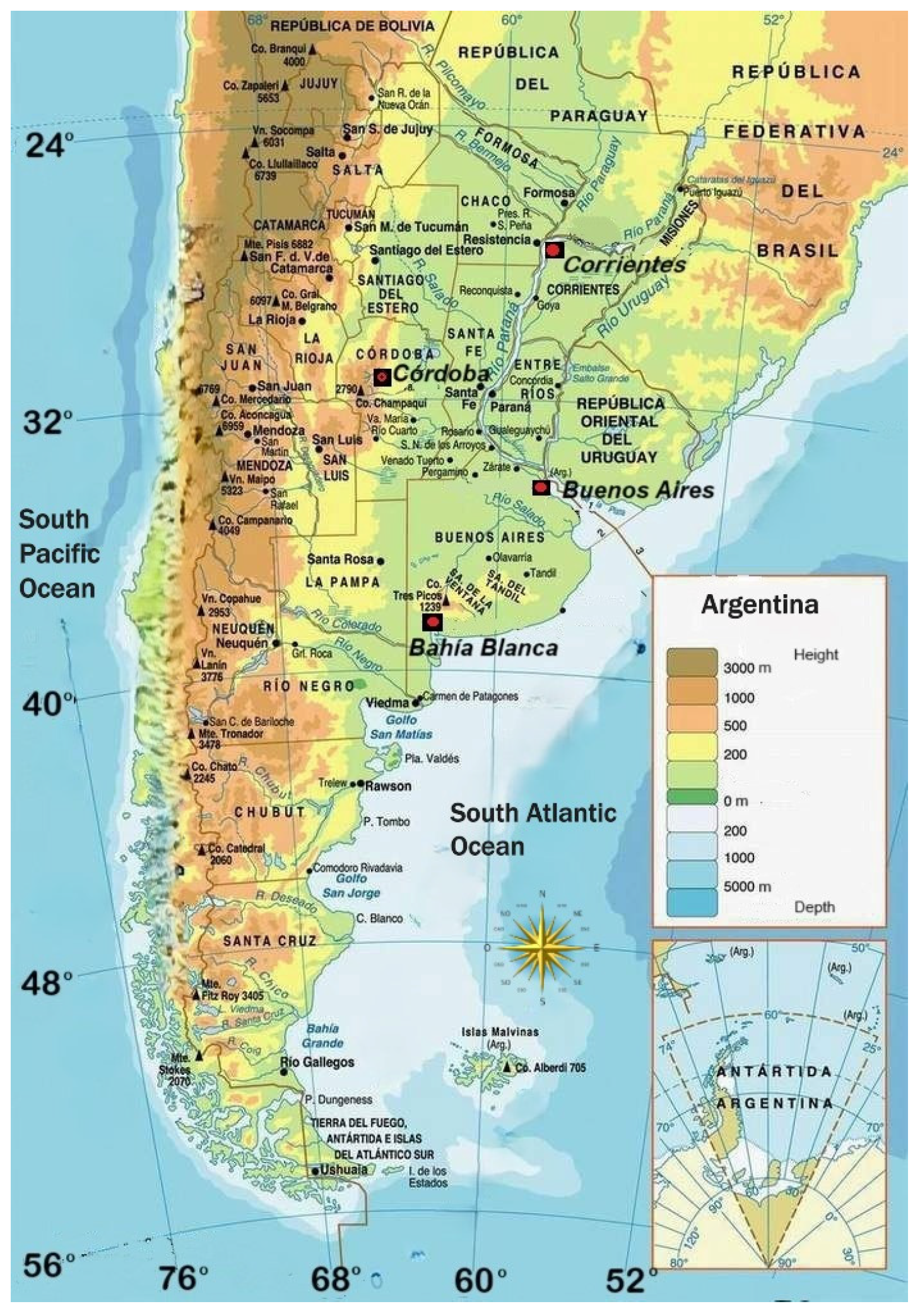
The 4 longest monthly precipitation records currently available for Argentina were chosen for this study. These correspond to Bahia Blanca, Buenos Aires, Córdoba Observatory, and Corrientes. These locations span central eastern and northeastern Argentina as can be seen on the map in
Figure 1. Corresponding geographical coordinates, climate regimes, and the beginning and end dates of each timeseries are given in
Table 1. The four locations have distinct climate regimes. The records were reconstructed from the GHCN-M database [
29] and data from Anales de la Oficina Meteorológica Argentina (OMA) published between 1878 and 1915, which contain information for 1860 to about 1910 daily and/or monthly mean precipitation, depending on the station. In all cases, there were very few missing months, and these were interpolated by linear regression as in Scian and Pierini [
20]. Thus, the longest record, corresponding to Bahia Blanca, covers the period from January 1860 through December 2023, i.e., 164 years. The shortest record in this study corresponds to Corrientes, spanning 148 years. It must be noted that the Córdoba Observatory records correspond to the first official weather station operated by OMA in Argentina, starting in 1873, with observations strictly following the International Meteorological Organization (IMO, later WMO) observation practices. Bahia Blanca and Buenos Aires fully complied with IMO requirements starting in 1873, though previous measurements are found to be reliable through statistical testing. Corrientes, starting in 1875, complied with IMO requirements from the beginning. Some years later, all of the records published by OMA included daily precipitation together with IMO weather symbols, so it is possible to determine, particularly in the case of significantly different monthly precipitation values, the kind of weather events that took place and, thus, validate extreme monthly precipitation values, if necessary, for the earlier decades of the samples. The complete procedure of data recovery and processing of the series can be found in Lakkis et al. [
30] among others, but briefly and in accordance with WMO recommendations [
31], the series were subjected to a quality control and tested for homogeneity [
32] using XLSTAT statistical software (2023.2.0). The Pettitt’s test, Alexandersson’s SNHT test, Buishand’s test (BRT), and von Neumann’s ratio test (VNRT) were used, considering a 5% significance level. The results derived from the applied homogeneity tests were interpreted by following the approach suggested by Wijngaard et al. [
33]. As a result of these tests, only the raw data for Córdoba were found to be homogeneous, while the rest of the series underwent a homogenization process as several breaks were detected between 1945 and 1965 (Corrientes between August and September 1945, Buenos Aires between November and December 1957 and Bahía Blanca between September and October 1965).
Monthly mean precipitation average values calculated for the period of 1903–2002 were used to obtain deseasonalised precipitation anomalies. Such an extended averaging period was selected, rather than the standard 30-year averaging, to take into account the considerable interannual to interdecadal variability observed in the precipitation timeseries. Furthermore, many official meteorological stations were established throughout the country during the first years of the 20th century; thus, such an averaging period is useful for intercomparisons with other stations in future studies. Deseasonalised timeseries were obtained by subtracting the 1903–2002 monthly mean precipitation for the corresponding month from the homogenised precipitation timeseries.
As pointed out by Anghileri et al. [
34], the detection of trends in timeseries of climate variables is often complex due to the seasonality and interannual variability that characterise natural systems. While seasonality behaviour can make the trend detection results strongly dependent on the selected time scale of analysis, interannual variability, meaning wide fluctuations from one year to another, can generate apparent trends, especially when the recorded timeseries are short. In order to identify annual, seasonal (DJF: summer; MAM: autumn; JJA: winter; and SON: spring), monthly, and anomaly precipitation trends, linear regression test, the nonparametric-based Mann–Kendall (MK), and the Sen’s slope estimator were used. These tools have been widely used for trend detection in a very wide variety of analyses, and a comprehensive review of the state of the art in these mathematical methods can be found in Kundzewicz and Robson [
35] and Sonali and Kumar [
36], among others.
Briefly, linear regression is a parametric test used to evaluate the pattern and trends of different variables measured over a long period of time. The test statistic is the slope of the least squares linear regression line divided by its standard error, and the rate of change in the series of data is defined by the slope [
36,
37].
The MK test compares relative magnitudes rather than the data values. The robustness of the MK test was highlighted in several studies [
38,
39] and has several advantages, such as being insensitive to outliers and missing data in timeseries. Estimated Z-scores are used to represent the magnitude of trends. The positive Z value infers a positive trend and vice versa. The significance level (α) used for the MK test of 0.05 (i.e., 95 percent confidence) is used to test the null hypothesis (no trend in the data). Finally, the Sen’s slope was considered to assess the magnitude of the trend [
40]. A positive value of Sen’s slope indicates an upward or increasing trend, and a negative value gives a downward or decreasing trend in the timeseries.
In order to further analyse the existence of significant decadal to interdecadal variability in the region, a rolling 60-month moving average or running average (which can be considered a low-pass filter),was applied to the timeseries to highlight the lower frequency variability. This 60-month running mean calculates the average of data points over a period of 60 months, where the average is recalculated as new data points become available and older ones are removed from the calculation. Essentially, a 60-month running mean is a dynamic average that tracks the trend in data over time, as opposed to a static average over a fixed period.
For the variability analysis, monthly and seasonal computed values of Southern Oscillation Index (SOI), the Niño3.4, the Pacific Decadal Oscillation (PDO), the IPO (Interdecadal Pacific Oscillation as represented by TPI), and the Atlantic Multidecadal Oscillation (AMO) indices, spanning all, if not most of the study period, were obtained from NOAA’s Physical Science Laboratory (
https://psl.noaa.gov/). While it would have been of interest to consider the Southern Annular Mode, at this time, there are no available validated extended timeseries prior to 1900 [
41]. An assessment of the correlation between those indices and precipitation values was performed with multiple linear regressions (MLR) using the XLSTAT 2024.3.0 software and considering all the climate modes as regressors.
Multiple linear regression was also applied to assess the dependence of the anomaly timeseries variability on the abovementioned climate indices. The method is well known enough in this type of analysis: in summary, the R2 coefficient retrieved indicates the % of variability of the dependent variable explained by the explanatory variables. Fisher’s F test used is less than 0.0001, which implies that a risk of less than 0.01% is implicit when assuming the null hypothesis. It can thus be confidently concluded that the variables shown in the best model provide a significant amount of information regarding the variability analysed, and graphical representation with the standardised regression allows us to directly compare the relative influence of the explanatory variables on the dependent variable, as well as their significance.
Finally, the analysis of the temporal behaviour of significant monthly anomalies or extreme events, both positive and negative, was carried out using monthly standard deviations, σ, as a normalisation factor. In this sense an extreme event can be defined when monthly anomalies ≥ σ. It is worth mentioning that the use of σ threshold is a direct measure of data dispersion around the mean, allowing for a statistically grounded approach to identifying outliers; therefore, it is a quantifiable way to define “unusual” values, with the number of standard deviations used reflecting a chosen level of confidence. While it is true that monthly precipitation anomalies have a skewed distribution, particularly for extreme positive events, it remains possible to use monthly σ to standardise the anomalies and, thus, obtain seasonal and complete normalised timeseries at each location. It must be noted that deciles were calculated for the complete and seasonal timeseries at each location. These yielded 90- and 10-percentile values in good agreement with the calculated monthly σ, 2σ, and 3σ. Furthermore, the standardisation with σ allows the intercomparison of significant events between locations. The total number of events per decade falling into each of these categories was determined, and their variations along the decades of the study period were considered, both for the full sample and seasonal samples.
3. Results
3.1. Monthly Precipitation Records
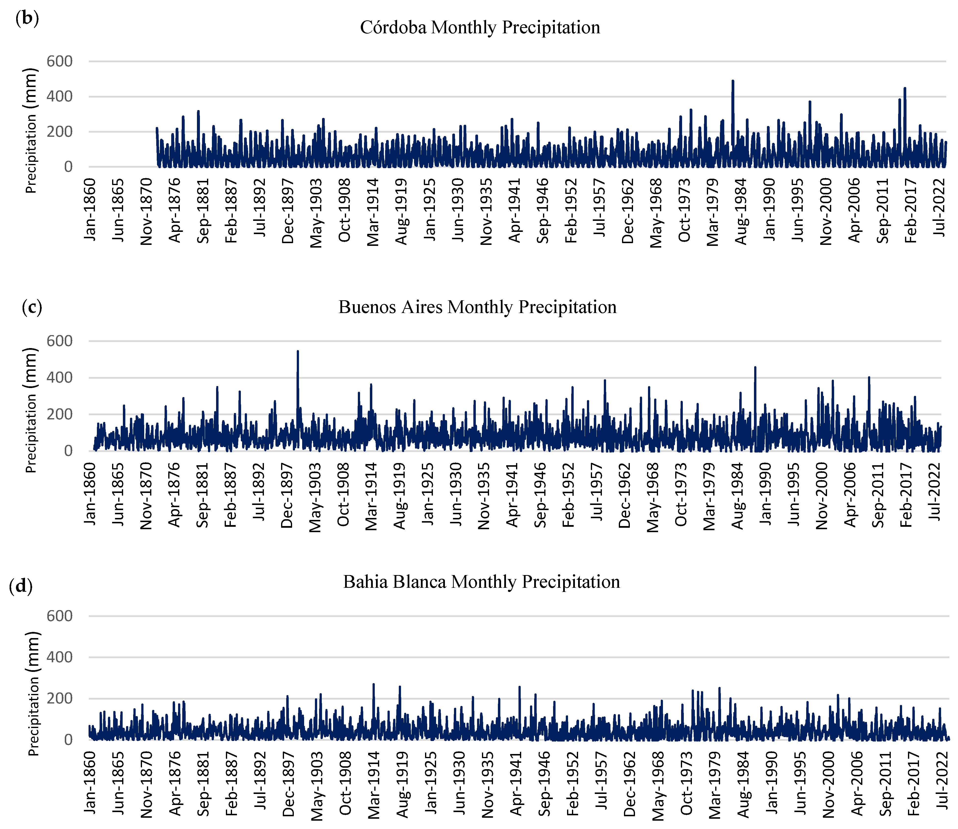
Figure 2 highlights the considerable variability in monthly precipitation at all four locations, as is to be expected. This variability can be observed not only from one month to the next but also over extended periods of time, i.e., years and decades. Clustering of high (low) monthly values can be observed along the timeline at all sites. Such clustering appears to take place at quasi-decadal/interdecadal periods, i.e., primarily early, mid, and late 20th century. This behaviour is further analysed in
Section 3.
At this point, it is interesting to consider the 5 rainiest months since the beginning of the records at each location.
Table 2 lists these months and the corresponding accumulated precipitation derived from the homogenised series. All the rainiest months, except for July 1940 at Corrientes, took place during the warm season, extending from November to April, during the austral late spring to early autumn. Only Córdoba has the top 5 rainiest months within the last 40 years. The earliest rainy month in Córdoba ranks 7th and dates back to December 1880. All other locations have the rainiest months distributed throughout the study period. It is interesting to note clusterings of very rainy months during the early decades of the 20th century and toward the end of the 20th century and early 21st century. A few such months also occurred in the mid-20th century. Furthermore, the rainiest months tend to occur more frequently in late summer and early autumn.
Daily precipitation values were obtained for the top-ranking months in Buenos Aires and Bahia Blanca, dating back to the early 20th century. During March 1900 [
40], Buenos Aires had 12 days with precipitation, 3 of them with considerable downpours in the vicinity of or exceeding 100 mm: 31 March 1900—135 mm, 28 March 1900—125 mm, and 29 March 1900—97.5 mm. Earlier in the month, on 11 March 1900, 55.5 mm had already precipitated over the city. Total precipitation was 544.5 mm. The worst daily precipitation for the period of 1861–2023 took place on 31 May 1985 with 188.4 mm. However, May 1985 ranks 13th (317.3 mm) when accumulated monthly precipitation is considered. For Bahia Blanca, the rainiest month on record (1860–2023) was April 1919, when the city endured 12 rainy days with a total precipitation of 314 mm. The worst precipitation took place on 9 April 1919 with 160 mm, 60 mm on the following day, and 66 mm on 12 April 1919. The rainiest day during the study period was 18 March 1933, with 167.7 mm daily precipitation. However, March 1933 accumulated 207 mm, i.e., the 12th rainiest month for Bahia Blanca during the study period. These examples, among others, highlight the fact that heavy monthly total precipitation (accumulated values over the month) may not necessarily be linked to the worst daily precipitation events, but rather to the number of significant precipitation events, particularly heavy precipitation ones, during a given month. In other words, record-high monthly precipitation points to the occurrence of a number of significant daily precipitation events during the month and/or sustained precipitation during an above-average number of rainy days. Such differences between extreme rainy months and severe single precipitation events should be taken into account when discussing the drivers of precipitation variability and changes.
It is worth looking back at some historic high precipitation episodes, which highlight the ever-present consequences of heavy rains. September 1884 is the 7th in the ranking of the rainiest months in Buenos Aires, with 349 mm of accumulated precipitation. On 23 September 1884, 118 mm precipitated, and on the following day, 127 mm precipitated [
42]. These significant storms resulted in considerable flooding of large areas of city, the consequences of which were inspected by the then President of the Republic, Julio A. Roca. Such an event resulted in the decision to move the cattle slaughterhouses located in the Parque Patricios neighbourhood to a then remote area, subsequently named Mataderos. However further heavy storms and flooding, particularly in January 1889 (rank 11th) with 324 mm of accumulated precipitation, 13 rainy days, and a 90 mm storm [
42], were necessary to confirm the determination to carry out the move, in 1901, during Julio A. Roca’s second presidency, and to advance in the construction of the huge precipitation drainage system for the city of Buenos Aires, completed in 1919.
3.2. Precipitation and Precipitation Anomaly Analysis
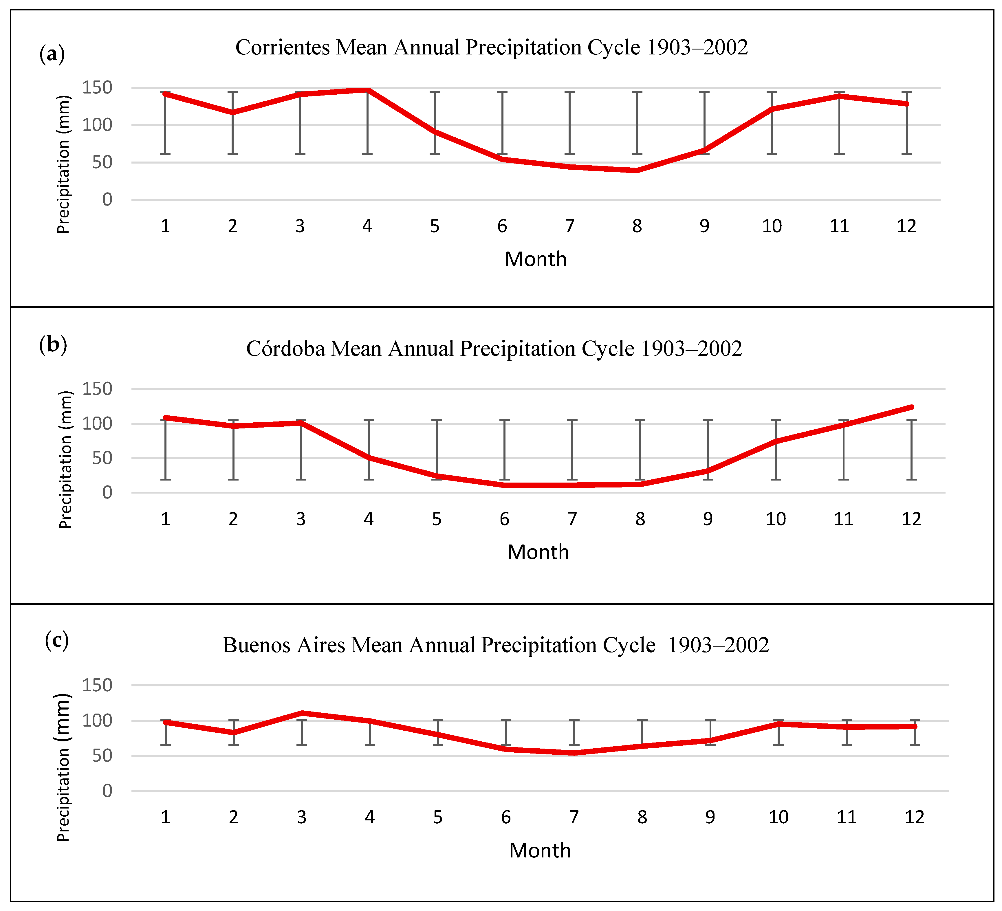
Figure 3 shows the annual precipitation cycles for the four locations where the distinct regimes at each location can be appreciated. Córdoba Observatory has a distinct seasonal variability corresponding to the South American Monsoon precipitation regime, i.e., rainy summers and very dry winters. Corrientes has a well-defined seasonal cycle, with heavy precipitation from October through April. Such behaviour at these two stations highlights the flow of humidity from the Amazon Basin brought in by the meridional South American low–level jet [
43,
44,
45] that enters Argentina’s Chaco and Pampas regions primarily between October and March. Buenos Aires precipitation, while still having a well-defined seasonal cycle, does not exhibit such large seasonal variations. Bahia Blanca, located by the South Atlantic, in the Yellow Pampas transition region between the humid Pampas and the Patagonian steppes’ semi-arid to arid climate, shows rather reduced precipitation, under 60 mm, with maxima in March and October.
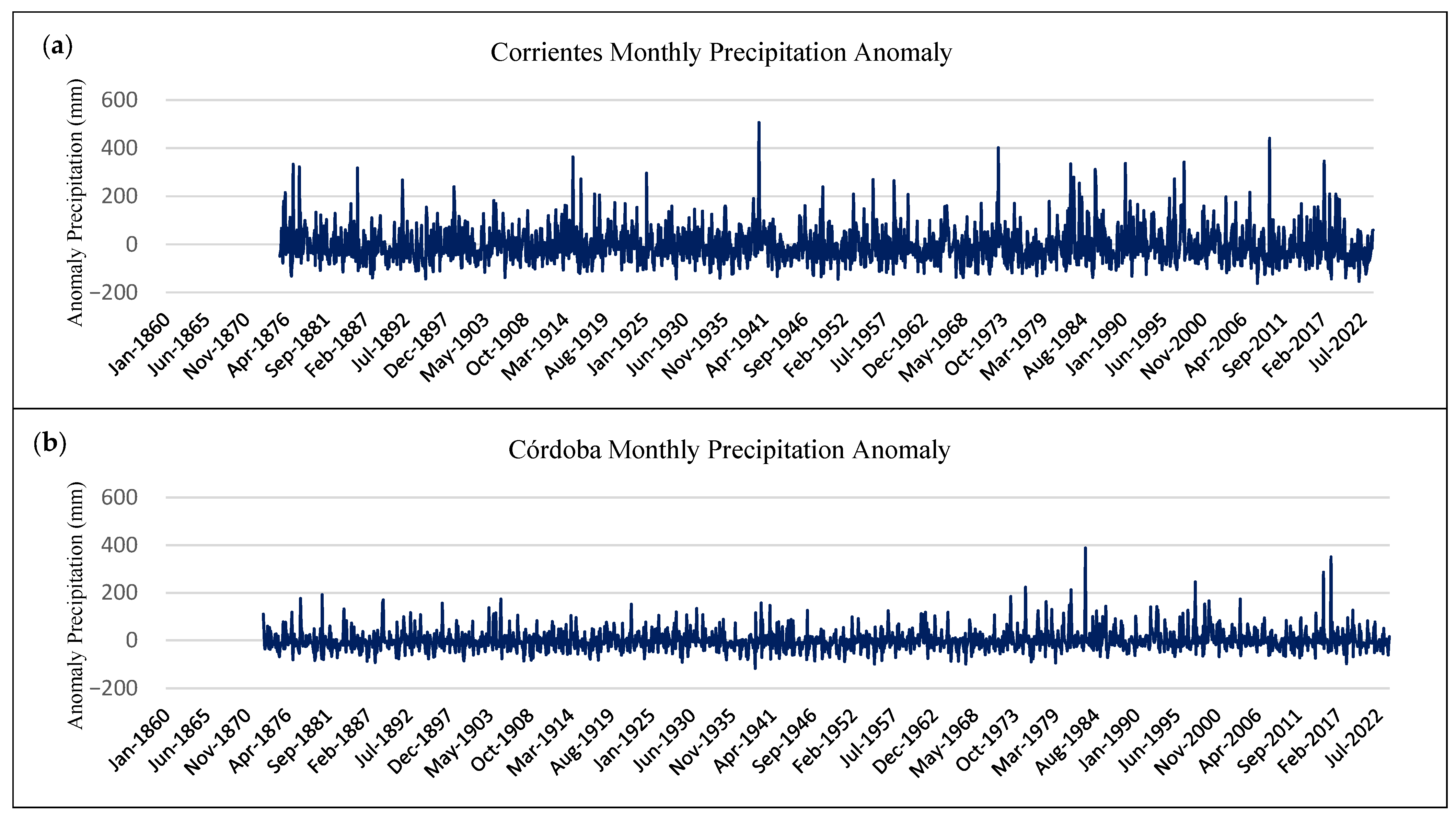
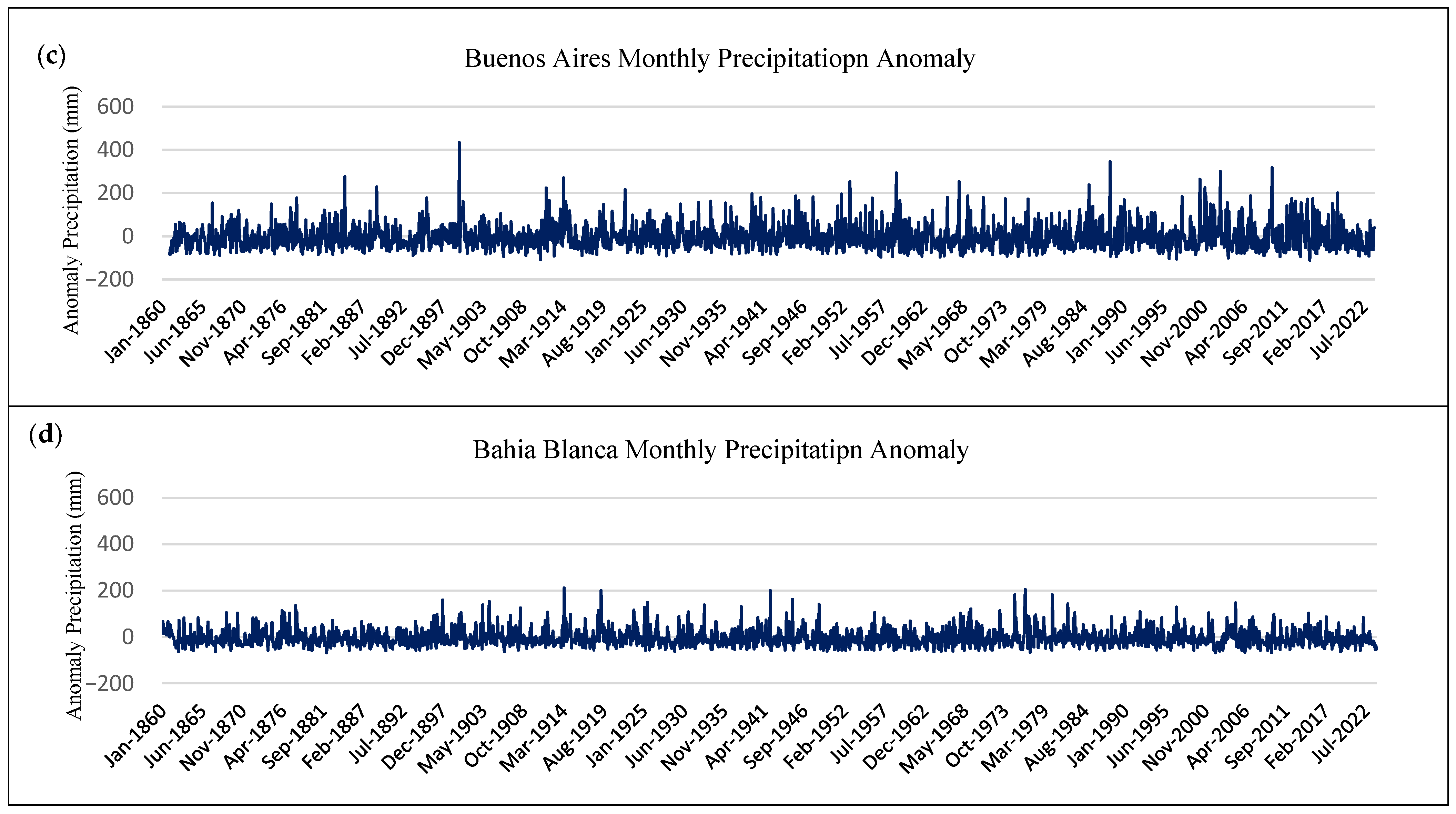
Figure 4 shows the deseasonalised precipitation anomalies at the four study sites, using the 100-year means presented in
Figure 3. Since the anomalies are deseasonalised, it is possible to compare the magnitude and evolution of monthly precipitations throughout the study period. Standardisation by the standard deviation further allows comparisons between stations.
A first inspection of
Figure 4 and its comparison with the homogenised precipitation series in
Figure 2 indicates some changes in the occurrence of extreme positive precipitation since the deseasonalisation impacts primarily occur during the warm months, during which precipitation maximises at all four stations. As a consequence, Corrientes, Buenos Aires, and, to a lesser extent, Bahia Blanca have fewer prominent maxima throughout and some changes in the ranking of the top rainiest months. The inspection of the Córdoba timeseries suggests that extremes, when deseasonalised, are not so prominent, particularly in the midsection of the sample, and negative anomalies appear to be more frequent, in agreement with De la Casa et al. [
21]. As before, the largest extremes have mostly occurred during the last 45 years.
The trend results for these four localities using MK test with the whole sample of homogenised data show that no trend can be detected—i.e., the null hypothesis cannot be rejected—in all cases, except in Bahía Blanca where a significant trend, albeit very slight, of the order of 0.003 mm per year, can be observed. The same conclusions are obtained from the linear regression and the Sen slopes (
Table 3).
Regarding the anomaly series, only a rather weak but significant trend (α = 0.05) was obtained for Córdoba. The calculated trend yields a 0.36 mm/decade increase in precipitation. This would imply an overall increase of 5.4 mm for the period of 1873–2023 in the deseasonalised anomaly timeseries. This result agrees with De la Casa et al. [
21] for the annual precipitation trend, albeit with a larger trend in their study. It is important to note that their results are based on the analysis of the samples beginning in 1910 at the earliest and finishing in 2010, i.e., 50 years less in the sample, which, furthermore, does not include the recent severe drought.
Figure 2 and
Figure 4 also show rather prominent monthly precipitation prior to 1910, as well as a few high monthly values after 2010. This has a significant impact on the trend calculation. On the other hand, Barros et al. [
19] and Camilloni [
17] found significant positive trends for the SESA region. However, it must be noted that they considered a far shorter timeseries, spanning the period of 1960–1999. Both
Figure 2 and
Figure 4 suggest that at least for Corrientes, Córdoba, and Buenos Aires, their study period coincided with years of enhanced and increasing precipitation in the region. As mentioned earlier in the methodology, according to Anghileri et al. [
34], the detection of trends in timeseries can be strongly influenced by the time period considered in the analysis. Furthermore, the differences between the results found may also be due to the processing of the data series. If the raw data of the four locations, analysed here (zenodo.org: DOI 10.5281/zenodo.15013403), without homogenisation, are considered, significant increasing trends are also observed in all cases except for Cordoba (where the null hypothesis cannot be rejected). However, as the WMO points out, results derived from a non-homogeneous dataset may be influenced by multiple extra-climatic factors, and therefore, trends cannot be considered conclusive or accurate.
Scian and Pierini [
20] demonstrated, using 40-year moving windows to study the return time of extreme dry and extreme wet conditions, the existence of significant decadal to interdecadal variability in the region. Similarly, De la Casa et al. [
21] found low-frequency interdecadal variability, with enhanced precipitation between the 1970s and early years of the 21st century for the stations they studied in the vicinity of Córdoba. Given that such trend differences depend on the sample length (
Figure 4), in agreement with Scian and Pierini [
20] and De la Casa et al. [
21], this suggests extended periods of heavy precipitation (positive anomalies) alternating with periods of reduced precipitation (negative anomalies).
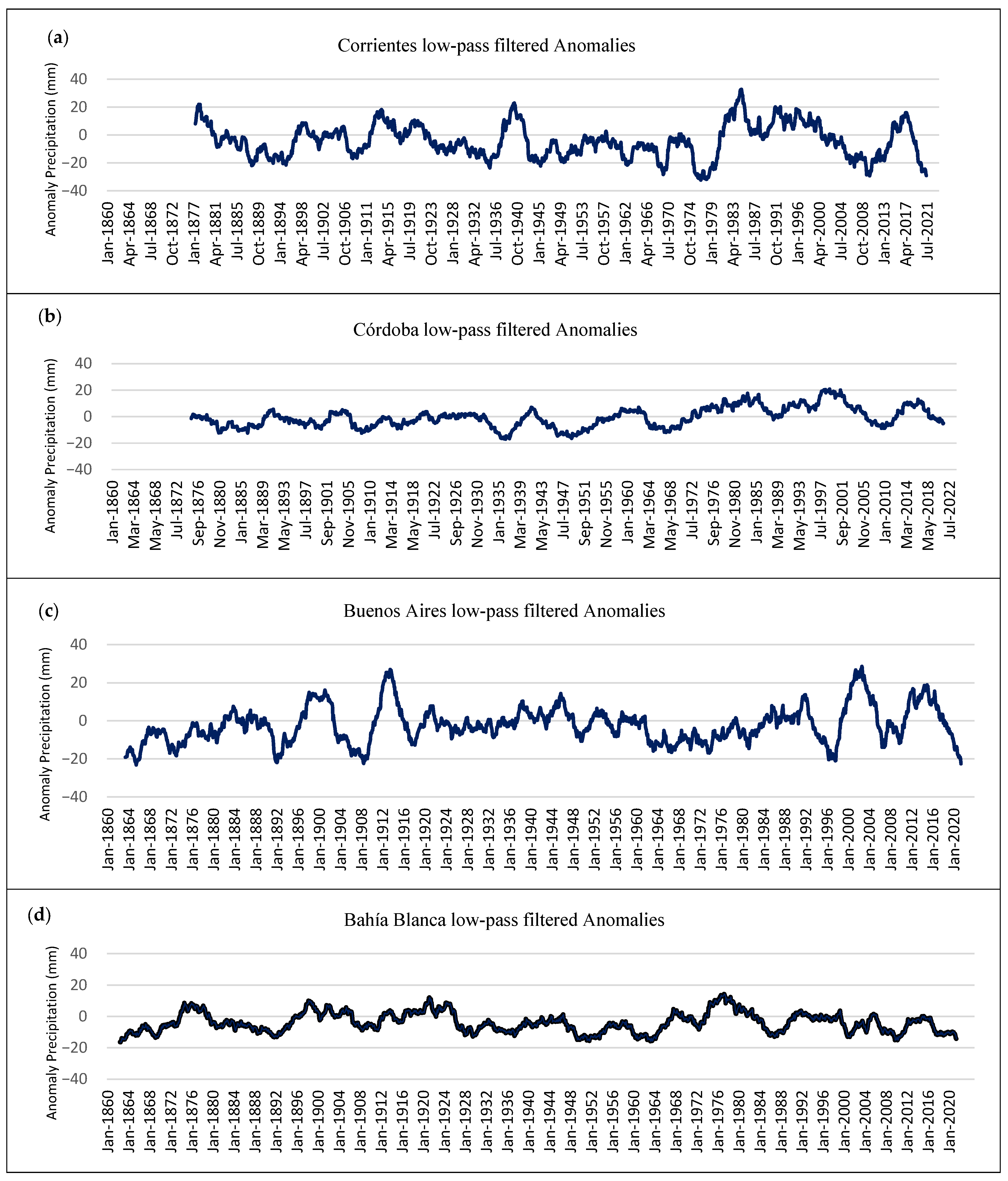
A 60-month (5-year moving window) was applied to the timeseries to highlight the lower-frequency variability.
Figure 5 shows the filtered anomaly time-series. Maximum positive low-frequency anomalies occurred at all stations during the last 50 years. Córdoba recorded its largest positive anomalies between the 1970s and 1990s. Corrientes precipitation maximised in the 1980s and, to a lesser extent, 1990s. Precipitation anomaly maximised in Buenos Aires later on, around 2002 and lasted only for a few years. Bahia Blanca reached a peak maximum anomaly in the 1970s. Another secondary maximum can be observed for Corrientes, Córdoba, and Buenos Aires in the period of 2012–2016. At this time, Bahia Blanca only shows a transition period with no significant anomalies separating the two dry spells. This could explain the positive trends found by many authors considering trends for timeseries spanning the last 40 or 50 years of the 20th century.
In previous decades, Córdoba did not show large/extended positive anomalies between 1873 and 1970. Buenos Aires had positive peaks around 1900 and 1910, while Bahia Blanca had positive low-frequency anomalies during the 1870s and in the period of 1890–1910. Corrientes, on the other hand, shows periods of positive values throughout the sample, more specifically the 1870s, 1910s and 1920s, and 1940s.
Regarding extreme dry periods, these vary considerably from station to station. Corrientes has its driest low-frequency spells in the late 1970s, between 2006 and 2012, and, finally, after 2017, a period during which the Paraná River almost dried up, particularly between 2022 and 2023. On the other hand, Córdoba underwent its driest spell in the 1930s and again between approximately 1945 and 1955. Other dry periods can be found in the 1880s and late 1910s to early 1920s. Dry spells in Buenos Aires occurred between 2018 to 2023 (record low), late 1990s, and prior to 1870, in the late 1890s and 1910s, during the earlier decades of the sample. It is interesting to note that during the years 1870 and 1871 when precipitation returned to what would be 20th-century average values, Buenos Aires, at the time without a drainage and sewer system, underwent a serious yellow fever epidemic that killed thousands [
46]. Finally, Bahia Blanca underwent its driest spells to date between 2018 and 2023, between 1860 and 1870, and in the 1910s. This region also suffered an extended period of almost continuous negative anomalies between 1930 and 1960. The dry spells, particularly for Bahia Blanca and Córdoba in the 1930s and 1950s, are in agreement with Seager et al. [
18].
Considering overarching aspects of the variability at these four stations, it must be noted that between 1976 and 1977, a major global climate transition, jump, or shift was observed, as documented by numerous authors. Mantua and Hare [
47] linked this abrupt climate shift to a rapid change of phase in the PDO. Agosta and Compagnucci [
48] identified the abrupt shift in Southern South America summer climate variables. Another climate regime shift and its consequences were observed in the early 1990s at least for the Southern Hemisphere [
49,
50,
51]. Regarding ENSO, Barrucand et al. [
41] noted that a wavelet analysis for three long-term ENSO indices (SOI, HADlSST Niño 3, and UKM GISST2.3 Niño 3) showed an almost complete disappearance of spectral power in the vicinity of 2- to 8-year period variability between 1920 and 1960. Such long-term behaviour could be at least in part responsible for the large positive anomalies observed in Corrientes and Córdoba during the last quarter of the last century.
To further analyse the possible role of ocean variability in precipitation at these four locations, a multiple linear regression (MLR) analysis was performed between the timeseries of precipitation anomalies and selected large-scale climate modes representing ocean variability, as mentioned above. It should be noted that here, we use the Niño3.4 and SOI indices, both of which are related to the ENSO signature. However, they represent different aspects of ENSO and ENSO teleconnections. The correlation between the two timeseries is 0.796, i.e., there are some differences. Similarly, while PDO is calculated using Northern Hemisphere EOFs of SST anomalies, TPI, an IPO proxy, considers EOFs of SST anomalies from both hemispheres. The correlation between TPI and PDO is 0.731. Again, there are some differences between these two indices. The MLR analysis (
Table 4) reveals that, when the best performing model is chosen, i.e., the set of climate indices and the linear modelling approach that best describe the behaviour of the precipitation anomalies, the total low-frequency variability explained in precipitation anomaly, for all four regions and for all the years, ranges from 5% to 16%. The highest percentage can be found in Corrientes, with 16% corresponding to AMO and TPI combined as main climate drivers. On the other hand, the lowest variability explained corresponds to Cordoba (7%), with AMO, Niño3.4, TPI, and PDO combined. Buenos Aires and Bahía Blanca display percentages of 10% and 12%, each corresponding to SOI-TPI and TPI-AMO indices, respectively. There is no noticeable correlation in the amount of rainfall variance explained with latitude; in fact, the only combination of mean drivers that is repeated corresponds to the two regions furthest from each other: Bahía Blanca and Corrientes. If a single model is used for each region over the entire analysis period, the variability explained decreases. Percentages of explained variability are overall in good agreement with the recently published values found in Hobeichi et al. [
24].
3.3. Seasonal Trends and Variability
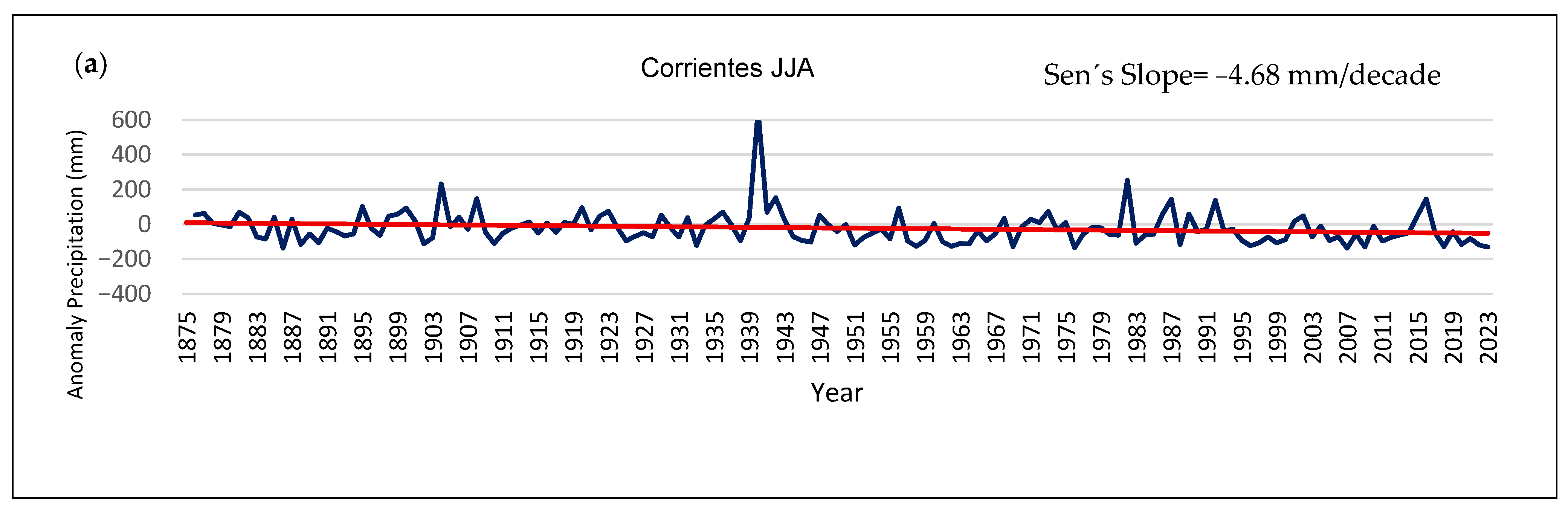
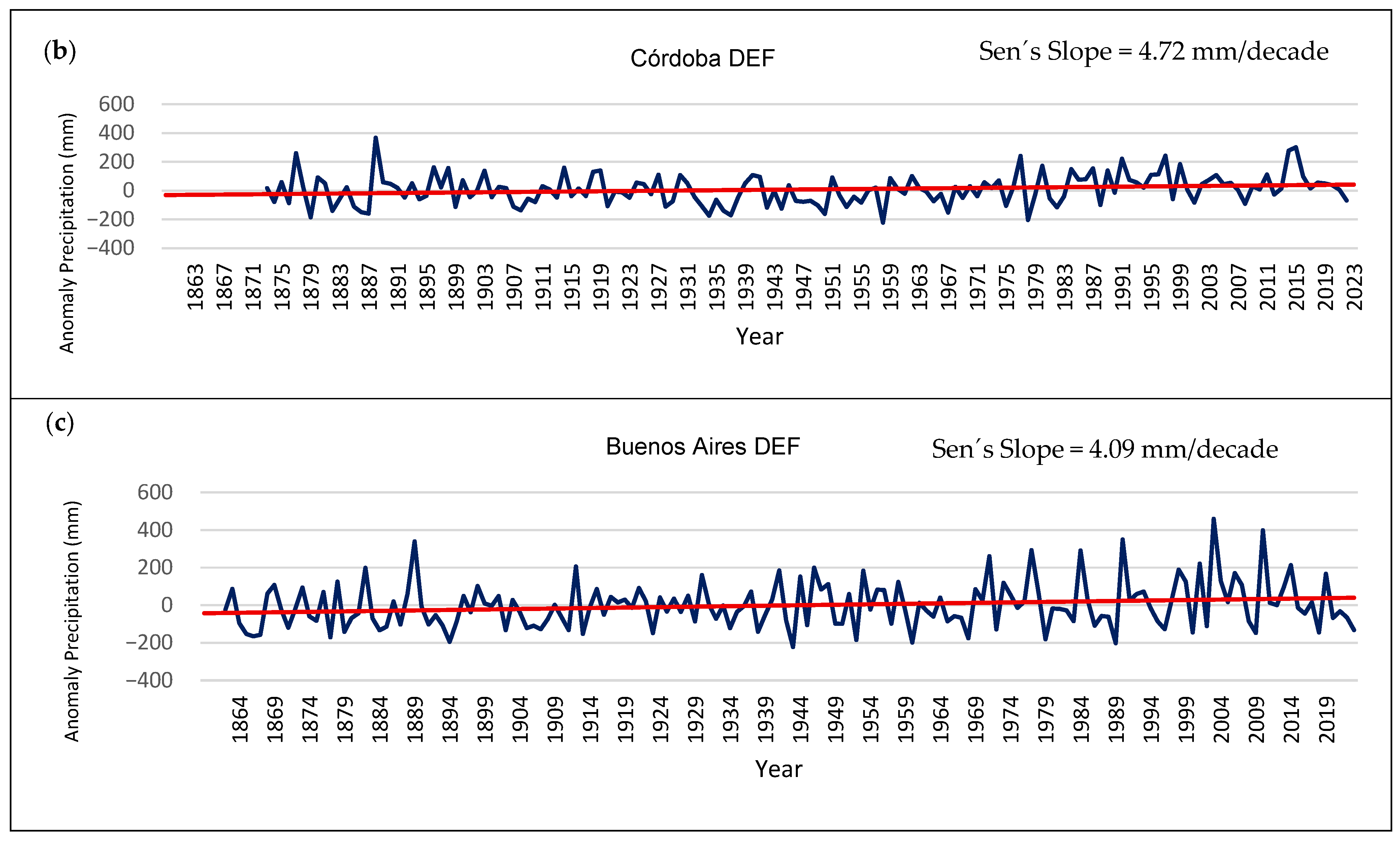
Precipitation is largely a warm-month climate feature in the region; thus, it is necessary to consider the seasonal evolution at each location to better understand trends and variability. Evaluation of the seasonal precipitation anomaly trends, using the MK test applied to each season’s anomaly rainfall data, shows that over the study period, there are a few statistically significant trends.
Table 5 presents the summary of the MK test results. Corrientes has significant negative trends during winter, while Buenos Aires and Córdoba have significant positive trends during summer between 1861 and 2023, with a 4.9 and 4.7 mm per decade precipitation increase.
Figure 6 shows the three cases with significant seasonal trends. The plots show that despite the existence of decadal to interdecadal variability, which is also present in all other seasonal anomalies with null trends, the trends obtained are a very good representation of the overall evolution of the seasonal precipitation anomalies during the study period.
To better understand how precipitation has varied in this region, the seasonal anomaly variability was tested. To explore this, MLR analysis with seasonal climate modes was used, and the results (
Table 6) show that, while the influence of these indices is relatively low when the whole period is considered, the seasonal variability in precipitation anomalies is considerably higher in some areas. For example, Corrientes shows explained variance around 29% linked to SOI, PDO, and TPI combined, during austral spring (SON), but the percentages are lower and even non-significant during all other seasons. A similar behaviour can be seen in Córdoba, where the amount of rainfall variance explained reaches about 16% in DEF (AMO and TPI), but for the rest of the seasons, the percentages decrease significantly. In the case of Buenos Aires, the minimum non-significant value corresponds to 2% in DEF, while the rest of the seasons display 7% of variability explained by different combinations of climate modes. Finally, Bahia Blanca has the maximum significant correlation between rainfall and climate modes, around 11% during JJA (TPI and ENSO represented by Ñiño 3.4 and SOI indices). Thus, the influence of climate modes on interannual and seasonal weather patterns appears to be similar, although with differences in the explained variance, with the Atlantic Multidecadal Oscillation and Tropical Pacific Influence being the dominant factors and the El Niño-Southern Oscillation playing a more minor role.
Comparing the influence of the indices on precipitation obtained here with results from other authors is a difficult task due to the scarce availability of analyses in Argentina involving such an extensive time period; however, the seasonal percentages found are, in general, in good agreement with Hobeichi et al. [
24].
3.4. Significant Monthly Deficits and Excess Precipitation Anomalies: A Perspective
Not only is it important to consider the trends and interannual to interdecadal variability of monthly/seasonal precipitation as given by the anomalies. It is also important to consider the deviations from the mean or, in this study, from the deseasonalised timeseries quasi-null mean. The distribution of significantly anomalous months (higher/lower than σ) along the approximately 150 years of the records considered is an integral part of the variability and trend analysis. As noted in the examples given above, the months with precipitation excesses must not be confused with individual severe precipitation events or days with extreme precipitation. This is more obvious when precipitation deficit periods are considered, i.e., dry periods and droughts are the known consequences of extended periods with little or no precipitation. It is also important to note that significant precipitation deficit months have been observed to occur side by side with significant precipitation excess months, further complicating the analysis.
As described above, these severe or extreme monthly anomalies will be described in terms of the standard deviation σi, where i is the month of the year used to standardise the corresponding monthly anomalies, represented by σ. Thus, anomalies become comparable between months, seasons, and locations. Using σi allows for the standardisation, resulting in the intercomparison of timeseries and visualisation through the quantification of the number of σ per range, as described in the methodology over selected periods of time, e.g., decades. Decades for the period of 1861–2020 are considered here.
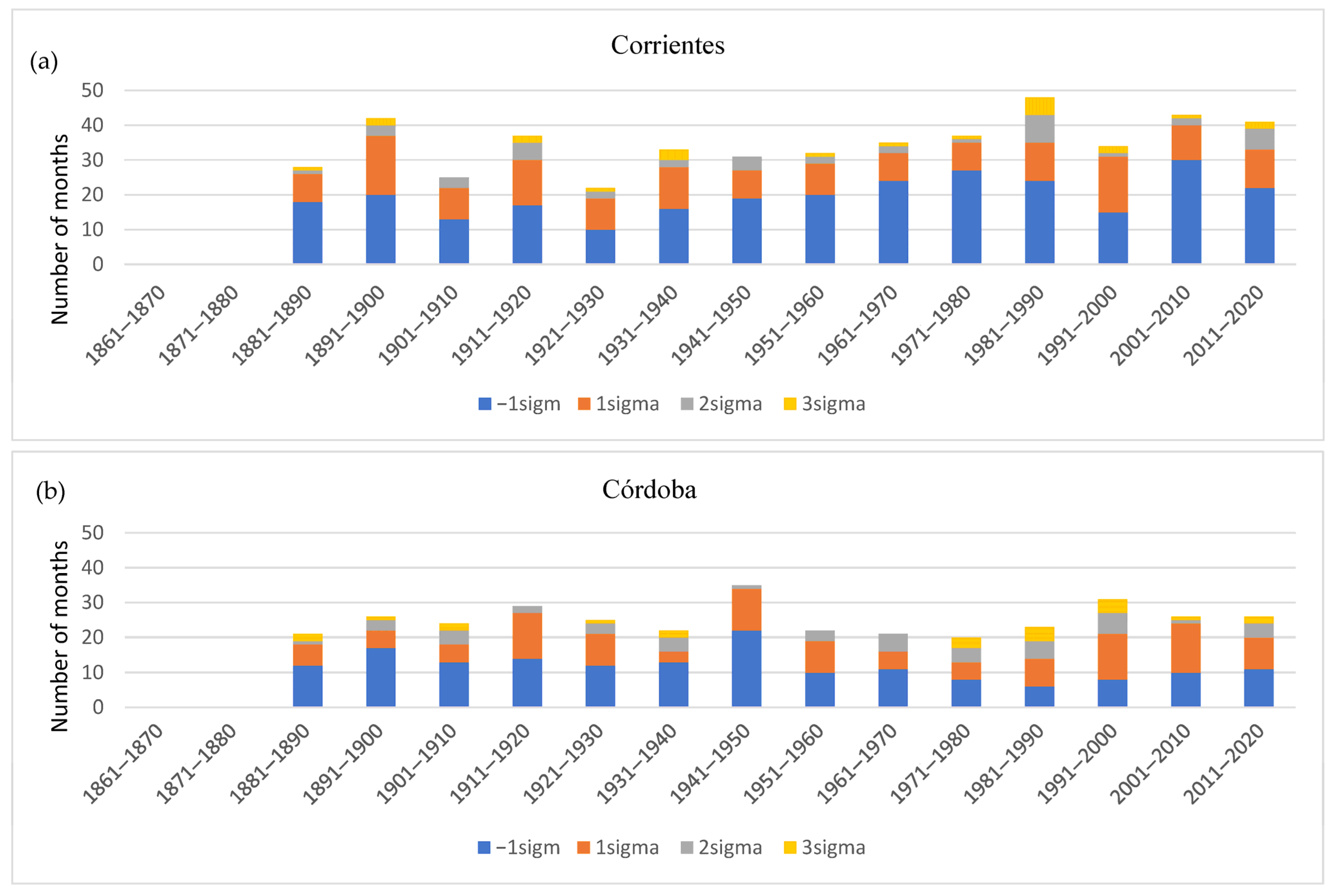
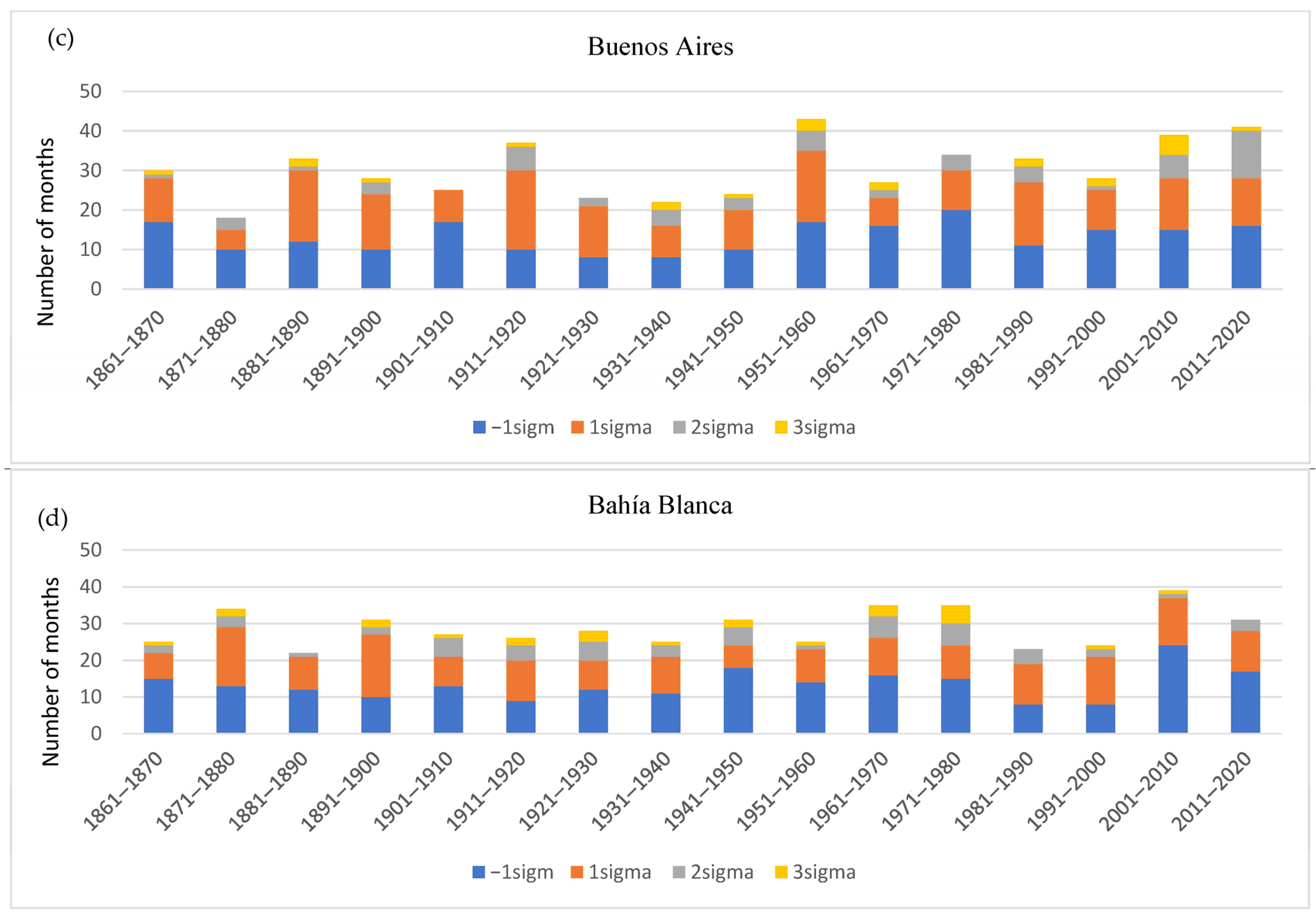
Figure 7 presents the decadal frequency distribution of σ per decade at each of the four locations. These histograms highlight the multidecadal variability of the four σ ranges (one negative, three positive) and are linked to the 60-month moving average results (
Figure 5) since low-frequency variations can modulate the parameters of the rainfall frequency distribution. Note that for precipitation deficit months, these all fall within a single range (−2 < σ ≤ −1), while excess precipitation months occur within an extended distribution tail, starting at 1σ and extending beyond 3σ. Overall, the number of months with significant precipitation anomalies per decade (both excess and deficit) oscillates between almost 17% and 42% of the sample size, depending on decade and location. Inspection of the histograms shows that at all four sites, almost all decades during the study period have at least one month with precipitation excess of at least 3σ. Bahía Blanca has a maximum number of such months during the period of 1971–1980 (5), while both Corrientes and Córdoba have such months maximised between 1981 and 1990 with 5 and 4 months, respectively. In the case of Córdoba, these do occur during the period with the largest precipitation anomalies. Buenos Aires has maxima of 3 such months twice in the sample, between 1911–1920 and 1951–1960. Further inspection shows that 3σ months variability has a recurrence of approximately 30 to 50 years for Corrientes during the 20th century, Córdoba 20 to 40 years, Buenos Aires 30 to 50 years, and Bahía Blanca 20 to 30 years. However, 2σ to 3σ months, which still represent months with significant precipitation excess, have fairly similar variabilities. As expected, 1σ to 2σ months are far more frequent. However, it is not as simple to pinpoint their variability, which exhibits significant variations throughout the study period at all stations. Similarly, the occurrence of months with significant precipitation deficit shows interdecadal variabilities that are difficult to pinpoint.
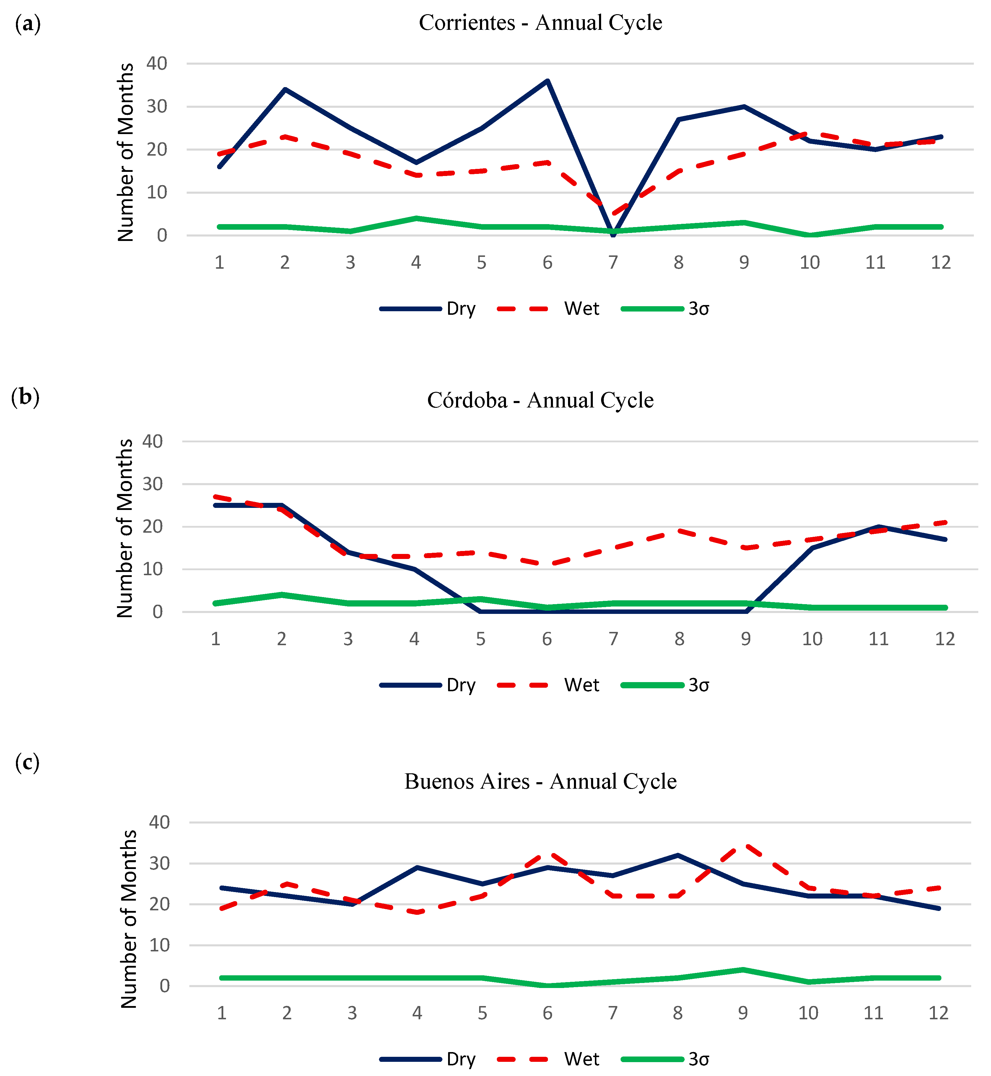
Figure 8 shows the accumulated annual distribution of significant anomalies for each month, for each station, i.e., accumulated during the full span of each sample. Briefly, 3σ months show few seasonal differences at all stations. In other words, such rare exceedingly wet months, given the size of the samples, have taken place throughout the year during the study period, with minor variability at some locations. On the other hand, when the total sum of all months with significant precipitation excesses is grouped by month, distinct seasonal cycles can be observed at each location. For Corrientes, significant months with anomaly precipitation excesses are maximised between September and April, during the warm period, with a minimum in July. Months with significant precipitation deficit are more frequent than months with excess precipitation, except during July, where a narrow and prominent minimum occurs. Deficit months are maximised in February, June, and September. For Córdoba, positive (wet) significant precipitation anomaly months occur more frequently in January and February, with somewhat lower values with limited variability from March to July, increasing after August, with a slow increase through December. On the other hand, significant negative (dry) anomaly months have a very well-defined annual cycle with practically no occurrences between May and September, i.e., during the cold season, in agreement with the very reduced mean precipitation during these months (
Figure 3b). These dry months are maximised during January, February, and November. During the warm period, the number of significantly wet and dry months is very similar. Buenos Aires has similar monthly counts for precipitation deficit and excess months. There is a very limited annual cycle: significantly dry months are somewhat more frequent during late autumn and winter, while months with significant precipitation anomalies are somewhat more frequent in winter and early spring. Bahia Blanca has a similar behaviour to Buenos Aires for significant excess precipitation months, while the annual evolution of the deficit months is fairly similar to Córdoba, with few if any significantly dry months during winter. Annual mean precipitation values in Bahia Blanca during winter are very similar to those obtained for Córdoba. Furthermore, the annual precipitation in Bahia Blanca is rather reduced when compared with the other three locations.
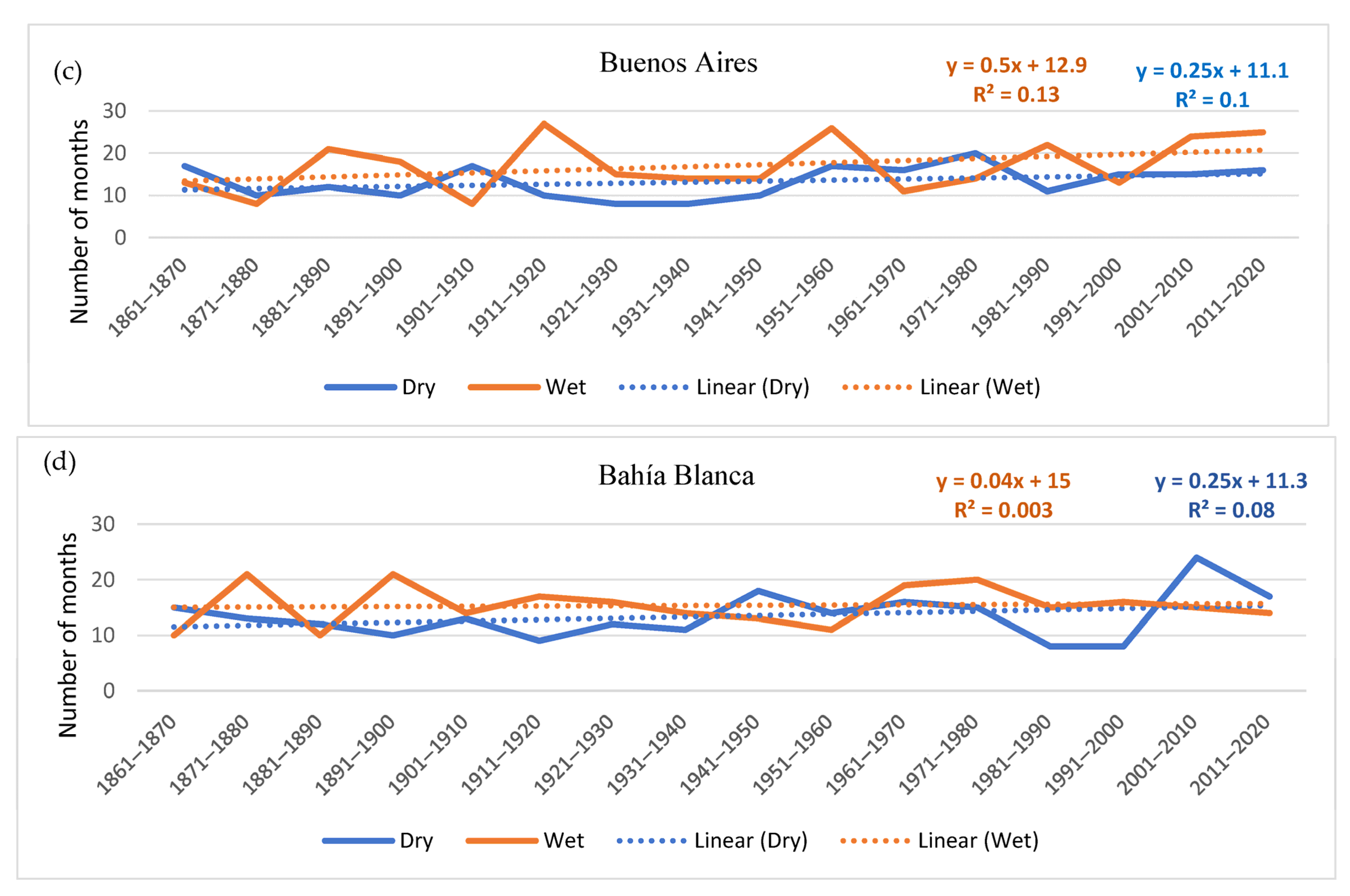
Figure 9 shows the evolution per decade of the total number of significant precipitation anomaly deficit and excess months at each location. Inspection of the plots shows different behaviours at each location. Considering the linear regression and MK test results, both Corrientes and Bahia Blanca have null trends for positive anomalies. While Corrientes appears to have a positive trend in the occurrence of significant negative anomaly months, Bahia Blanca has non-significant trends. Buenos Aires appears to have almost identical trends for negative and positive anomalies, i.e., the number of months with significant deficit or precipitation is slowly growing. Finally, Córdoba appears to have a positive trend in the number of months with significant excess precipitation and a negative trend for the months with deficit precipitation. Yet MK testing yields that all these apparent trends are, however, non-significant.
The seasonal anomaly trends at each of these locations once more suggest different behaviours at each of the locations and in different seasons. For Corrientes, significant excess precipitation months are weakly increasing during summer and autumn, decreasing during winter and spring, albeit non-significantly in all cases. Significant deficit months appear to be increasing during autumn, winter, and spring and decreasing in summer, once more non-significantly. Córdoba has, during summer, a positive trend for months with excess precipitation, as well as a decrease in significant deficit months. The rest of the seasons have non-significant positive or null trends for months with precipitation excess, as well as either non-significant decreasing or null trends for months with precipitation deficit. Buenos Aires only yields trends during summer and winter months, respectively: during summer, the number of significant excess precipitation months is increasing, while the number of precipitation deficit months is increasing during winter months. Bahia Blanca has null trends for all seasons, except summer. During these seasons, the number of dry and rainy months has a weak positive yet non-significant trend.


