Abstract
The introduction of the ”dual carbon” target has increased the need for products that can accurately measure carbon dioxide levels, reflecting the rising demand. Due to challenges in achieving the required spatiotemporal resolution, accuracy, and spatial continuity with current carbon dioxide concentration products, it is essential to explore methods for obtaining carbon dioxide concentration products with completeness in space and time. Based on the 2018 OCO-2 carbon dioxide products and environmental variables such as vegetation coverage (FVC, LAI), net primary productivity (NPP), relative humidity (RH), evapotranspiration (ET), temperature (T) and wind (U, V), this study constructed a multiple regression model to obtain the spatial continuous carbon dioxide concentration products in the provinces of Huai River Basin. Using indicators such as correlation coefficient, root mean square error (RMSE), local variance, and percentage of valid pixels, the performance of model was validated. The validation results are shown as follows: (1) Among the selected environmental variables, the primary factors affecting the spatiotemporal distribution of carbon dioxide concentration are ET, LAI, FVC, NPP, T, U, and RH. (2) Compared with the OCO-2 carbon dioxide products, the percentage of valid pixels of the reconstructed carbon dioxide concentration data increased from less than 1% to over 90%. (3) The local variance in reconstructed data was significantly larger than that of original OCO-2 products. (4) The average monthly RMSE is 2.69. Therefore, according to the model developed in this study, we can obtain a carbon dioxide concentration dataset that is spatially complete, meets precision requirements, and is rich in local detail information, which can better reflect the spatial pattern of carbon dioxide concentration and can be used to examine the carbon cycle between the terrestrial environment, biosphere, and atmosphere.
1. Introduction
The concentration of carbon dioxide in the atmosphere, accounting for approximately 0.04% of the total atmospheric composition [1], poses a significant threat as a greenhouse gas, ranking second only to water vapor. The concentration of carbon dioxide is 50% higher than that in the pre-industrial era, trapping heat in the atmosphere. Because carbon dioxide has a long lifetime in the atmosphere, temperatures will continue to increase in the coming years [2]. Since the reform and opening-up, China’s economic development has accelerated, and the country has now become the world’s second-largest economy, a leader in green economy technology, and has expanding global influence. In 2020, based on the inherent requirements of promoting sustainable development and the responsibility of building a community with a shared future for mankind, China announced the goal of carbon peaking and carbon neutrality [3]. To achieve the goal of “double carbon”, it is necessary to accurately monitor and evaluate carbon sources and sinks.
Currently, carbon dioxide data are obtained from ground-based, space-based observations and model simulations. It is difficult to describe the spatial distribution characteristics of regional carbon dioxide concentrations due to the scarcity of global ground-based sites. The reliability of the model simulation concentration is uncertain. Satellite observations have become one of the most effective means of monitoring global greenhouse gas emissions with high spatial and temporal resolution [4], and have improved human insight into the global distribution of carbon dioxide [5]. However, the spatial resolution of satellite products is relatively low, with spatial resolutions of 30 km, 10 km, 7 km, 2.5 km, 1.5 km, and 2.5 km for SCIAMACHY (Scanning Imaging Absorption Spectrometer for Atmospheric CHartographY, European Space Agency (ESA), Paris, France), GOSAT (Greenhouse Gases Observing Satellite), GOSAT-2, GOSAT-GW (Greenhouse Gases and Water Cycle Observation satellite), OCO-2, and TanSAT (Global Carbon Dioxide Monitoring Science Experiment Satellite), respectively [6]. The number of valid pixels is relatively low. In our study area, the proportion of the monthly average valid pixels of OCO-2 in 2018 was only 0.49%. The different satellite products lack physical consistency owing to the differences in inversion algorithm. For example, the Differential Optical Absorption Spectroscopy (DOAS) algorithm, the Weighting Function Modified DOAS (WFM-DOAS) algorithm, and the Band-Enhanced Sensitivity Differential (BESD) algorithm used by SCIAMACHY, the ACOS (Atmospheric CO2 Observations from Space) XCO2 inversion algorithm used by TANSAT, and the combination of high-resolution spectroscopic measurements and advanced inversion techniques used by OCO-2.
Many studies have reconstructed and simulated regional or global atmospheric concentration by simulating the relationship between atmospheric concentration observed by satellites and environmental variables. To solve the problem of missing values in single-source satellite products, the current main methods are the kriging spatiotemporal interpolation method [7,8,9], regression method [10], artificial neural network method [11], and high-precision surface modeling method [12]. Both kriging spatiotemporal interpolation and high-precision surface modeling methods are susceptible to the influence of the number and distribution of effective observations. The more effective measurement quantities there are and the more evenly the distribution is, the better the simulation effect is. In areas with sparse effective observations, the interpolation uncertainty was large. The interpolated data have strong continuity, but the data are smooth and lack local details. The current method for the fusion of multi-source data is relatively simple, for example, the multi-source data averaging method [13,14]. When multi-source data are averaged based on a certain spatial resolution, the global spatial coverage of the fused dataset can be improved by 20% and the temporal resolution can be improved by two to three times. For example, several months of GOSAT and SCIAMACHY data were integrated, but there were still missing pixels and spatial discontinuity [13,14]. In the future, more ground-based observations are needed to integrate multi-source satellite-derived data, especially data from China’s Carbon Satellite (TANSAT) [15], to study the fusion methods and theories for multi-source products.
The spatial distribution of was found to be related to the vegetation index, net primary productivity, leaf area index, atmospheric temperature, and wind [5,10,11,16]. Research results have shown that land surface parameters can be used to simulate atmospheric concentrations [5]. Environmental variables, especially spatial pollution data, are closely related to human health. By linking them through advanced modeling, the motivation for improved reconstruction is reinforced [17].
In the past 100 years, changes in vegetation and concentration have led to a trend of aridity in some areas of East Asia, especially in the Huai River Basin, Shandong Peninsula, and Yunnan. Therefore, to resolve the problem of missing values in single-source satellite products, in this study, a multiple environmental variable regression analysis method was used to reconstruct spatially continuous atmospheric concentration data in the provinces of Huai River Basin, China in 2018. First, several environmental variables, such as vegetation coverage, relative humidity, evapotranspiration, temperature, and wind, were selected. The correlation between the OCO-2 concentration and each environmental variable was evaluated. Variables with high correlation were selected, and collinearity analysis was conducted to determine the regression variables. The OCO-2 concentration and environmental variables were resampled to a fine resolution, a regression model was constructed, and the spatially complete concentration in the study area was obtained.
This study aimed to construct a regression model based on multiple environmental variables and obtain a spatially continuous monthly carbon dioxide concentration dataset for the study area in 2018. The remainder of this paper is organized as follows. The details of the datasets used in this study and the procedures for datasets preprocessing are provided in Section II. In this section, we also describe the regression model based on multiple environmental variables that was developed in this study. Section III demonstrates the implementation of the methods developed for the OCO-2 products. The final section summarizes the conclusions of our study.
2. Material and Methods
2.1. Study Area
The study area includes five provinces in the Huai River Basin in eastern China, as shown in Figure 1. It is an important economic and agricultural region in China. These provinces include Shandong, Anhui, Jiangsu Henan, and Hubei, with a total area of approximately 270,000 square kilometers. The terrain is higher in the west and lower in the east. The west is mainly composed of mountainous and hilly areas, whereas the east is a vast plain. The Huai River Basin has a warm temperate monsoon climate. Here, summer is the primary rainy season and the season with the highest temperatures. The average annual precipitation in the basin is 880 mm, and precipitation increases from west to east. The average annual temperature in the basin ranges from 13.2 °C to 15.7 °C, with a high temperature in the south and low temperature in the north. The annual relative humidity ranges from 66% to 81%. The main crops are wheat, rice, corn, potato, soybean, cotton, and canola (http://www.mwr.gov.cn/szs/hl/201612/t20161222_776385.html, accessed on 17 February 2025). As an important agricultural and industrial area in China, the Huai River Basin has a significant impact on the country’s economic development and ecological balance.
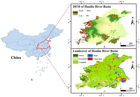
Figure 1.
Location and spatial distribution of elevation, land cover of the study area ((a): location; (b): elevation range; (c): land cover).
2.2. Data and Preprocessing
The data used in this article include OCO-2 products, vegetation coverage (FVC), leaf area index (LAI), net primary productivity (NPP), evapotranspiration (ET), temperature (T), relative humidity (RH) and wind (U, V) (Table 1).

Table 1.
OCO-2 and environmental variables used in this study.
2.2.1. OCO-2 Products
The NASA OCO-2 satellite was launched in July 2014 and was equipped with three high-resolution spectrometers. It monitors sunlight reflected from the Earth’s surface in the 0.76 μm A-band and the 1.61 μm and 2.06 μm bands to generate the column-averaged dry air mole fraction of () [18,19,20]. The OCO-2 observation data in this article are sourced from https://oCO2.gesdisc.eosdis.nasa.gov/data/OCO2_DATA/ (accessed on 13 January 2025) and the spatial resolution is 2.25 × 1.29 km, with a temporal resolution of 16 days. There were 351 scenes in the study area in 2018.
2.2.2. Environmental Variables
The concentration of carbon dioxide in the atmosphere is influenced by meteorological conditions, vegetation, and moisture levels, resulting in diverse and complex variability [21]. In the selection of environmental variables affecting the concentration of , eight influencing factors in three categories of vegetation structure, vegetation function, and meteorological conditions were considered, including Fractional Vegetation Cover (FVC), Leaf Area Index (LAI), Net Primary Productivity (NPP), Evapotranspiration (ET), Air Temperature (T), Relative Humidity (RH), and 10-m wind components (U, V). The FVC, LAI, NPP, and ET data were obtained from the GLASS data website (http://www.glass.umd.edu/Download.html, accessed on 13 January 2025). The spatial resolution for FVC, LAI, and NPP was 500 m, while that for ET was 1000 m. The temporal resolution of all these data was 8 days. The data of air temperature at 2 m, relative humidity, and the eastward and northward components of the 10 m wind were obtained from the ERA5 reanalysis dataset (https://cds.climate.copernicus.eu/, accessed on 13 January 2025). The data format was NetCDF with a monthly temporal resolution and a spatial resolution of 0.25 degrees.
2.3. Data Preprocessing
2.3.1. Data Preprocessing
First, the quality control of the data products was performed. High-quality data with QF = 0 [22] were selected. GLT correction was then carried out, and it was calibrated to WGS84 coordinates with a spatial resolution of 0.01°, then cropped to the Huai River Basin, and the monthly data were generated by the maximum value synthesis method (MVC).
2.3.2. Environmental Variables Preprocessing
The MODIS Reprojection Tool (MRT) was used to batch-process FVC, LAI, NPP, and ET data on a monthly basis and project them onto the WGS84 coordinate system to ensure their suitability for analysis. The spatial resolution was resampled to 0.01° and the data were cropped accordingly.
The technical process is illustrated in Figure 2. Some of the processed data are presented in Figure 3.
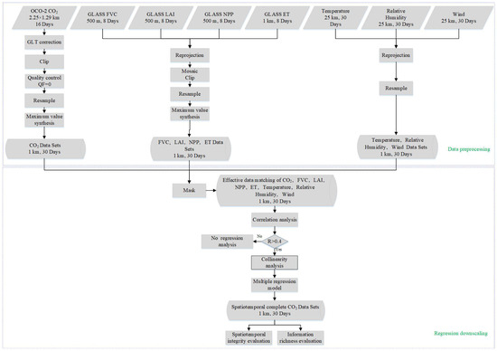
Figure 2.
Flowchart of the proposed downscaling framework for generating spatiotemporally complete fine-scale .
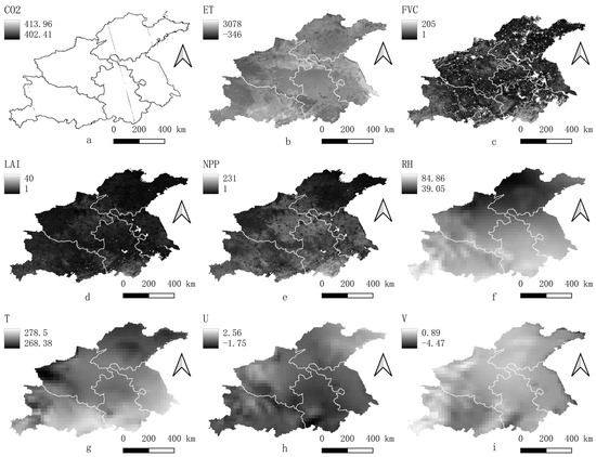
Figure 3.
Spatial pattern of a portion of the processed OCO-2 and environmental variables data ((a): OCO-CO2; (b): ET; (c): FVC; (d): LAI; (e): NPP; (f): RH; (g): T; (h): U; (i): V).
2.4. Statistical Methods
In this section, the methodology used in this study is described. It mainly includes two methods: univariate regression analysis, which is used to describe the correlation between carbon dioxide concentration and individual environmental variable factors and multivariate regression analysis, which is used to obtain spatially complete fine-scale carbon dioxide concentration data.
2.4.1. Correlation Analysis Method
The Pearson correlation coefficient, denoted as r, quantifies the extent of the linear association between two continuous variables (Formula (1)). In this study, the correlation coefficient was employed to screen environmental factors.
where r represents the correlation coefficient between the two variables, and its value ranges from −1 to 1. When , it indicates a positive correlation, that is, the two variables are correlated in the same direction; when , it indicates a negative correlation, that is, the two variables are correlated in different directions. The closer the absolute value of r is to 1, the closer the relationship between the two variables is. The closer r is to 0, the less closely related are the two variables. When the absolute value of the correlation coefficient r is (0 0.1], (0.1 0.4], (0.4 0.6], (0.6 0.9], and (0.9 1], the correlation degree is very weak, weak, moderate, strong, and extremely strong, respectively [23].
2.4.2. Multiple Linear Regression Analysis
The multiple linear regression model is a statistical method used to study the linear relationship between two or more independent variables (explanatory variables) and one dependent variable (response variable) (Equation (2)). Its purpose is to predict or explain the variation in the dependent variables from the independent variables. In this study, environmental variables that exhibited a strong linear relationship with the dependent variable, concentration, were selected to construct a spatiotemporal model of the concentration in the Huai River Basin for the 12 months of 2018.
Here, represents the dependent variable, which in this study is the concentration; ) represents the independent variables, which in this study are the environmental variables; ) represents the regression coefficients, which are estimated using the method of least squares; represents the residual, which follows a normal distribution [22].
3. Results and Discussion
Based on the method suggested in the Section Material and Methods, the correlation between the OCO-2 carbon dioxide concentration and a single environmental variable was analyzed, and a multiple regression model of carbon dioxide concentration based on multiple environmental variables was constructed. A fine-scale carbon dioxide concentration product with spatial and temporal integrity was obtained.
3.1. Exploratory Data Analysis
MATLAB R2020a was used to read the image data, create a validity mask to identify all non-zero and non-empty pixel values as valid pixels, filter out the data of each environmental variable at the positions of valid pixels using a logical index, and calculate the monthly mean of the valid data. Table 2 shows the monthly mean OCO-2 and environmental variables. Figure 4 shows the changing trend between OCO-2 and the individual environmental variables. The OCO-2 and environmental variables maintained similar changing trends. From April to July and from September to December, the two changed in opposite directions, except for the U and V.
Table 2.
Monthly mean values of OCO-2 concentration and environmental variables.
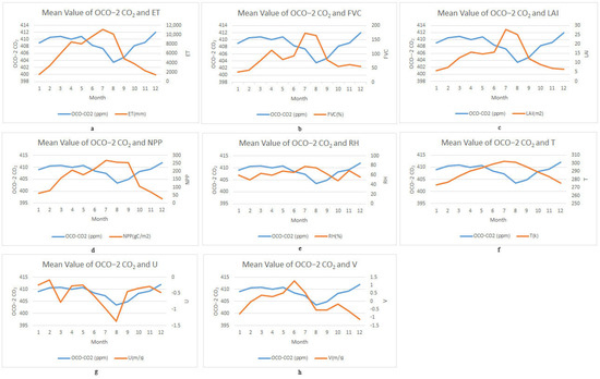
Figure 4.
Changing Trend between the OCO−2 and environmental variables ((a): OCO−2 and ET; (b): OCO−2 and FVC; (c): OCO−2 and LAI; (d): OCO−2 and NPP; (e): OCO−2 and RH; (f): OCO−2 and T; (g): OCO−2 and U; (h): OCO−2 and V).
3.2. Correlation Analysis
A correlation analysis was performed between the concentration and eight environmental variables to explore the relationship between the CO2 concentration and variables. The results are presented in Table 3. The results show a significant linear relationship between FVC, LAI, T, U, and the concentration. The linear relationship between ET, NPP, RH, and the concentration was not obvious, but there was no correlation between V and the concentration.
Table 3.
Correlation analysis results between concentration and environmental variables.
3.3. Multiple Linear Regression Model Construction
Before selecting independent variables whose absolute value of correlation coefficient with the dependent variable concentration was greater than 0.4 (i.e., ET, FVC, LAI, R, T, and U) to participate in the construction of the multiple linear regression model, a collinear analysis was performed. The results are presented in Table 4. As shown in Table 4, there is severe collinearity between the independent variables FVC and LAI. Therefore, the FVC with a higher correlation with the was selected to participate in the construction of the regression model.
Table 4.
Results of multiple linear regression and collinearity analyses.
Multiple linear regression analysis was performed on the readjustment variables. The coefficients of the model are presented in Table 5. The regression equation was found to be significant with an adjusted R2 of 0.404, indicating that the selected five independent variables explained 40.4% of the variation in concentration. The Variance Inflation Factor (VIF) values were significantly reduced, indicating that there was no severe multicollinearity among the independent variables, and the regression results were reliable.
Table 5.
Multiple linear regression results after adjusting for variables.
According to the results in Table 5, the multiple regression equation for the concentration can be obtained (Formula (3)):
where is the concentration of , , , , , , and are ET, FVC, NPP, RH, T, and U, respectively.
3.4. Comparative Analysis of Original OCO-2 Satellite and Reconstructed Data
According to Formula 3, based on the spatially complete satellite environmental variables FVC, T, U, ET, and RH, the spatially complete concentration data with 1 km spatial resolution for 12 months in 2018 in the study area were obtained. The spatial distribution of the reconstruction data is shown in Figure 5.
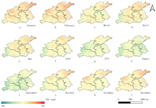
Figure 5.
Spatial pattern of monthly reconstructed concentration at fine-scale in 2018 ((a): January.; (b): February; (c): March; (d): April; (e): May; (f): June; (g): July; (h): August; (i): September; (j): October; (k): November; (l): December).
There was significant regional and temporal heterogeneity in the distribution of reconstructed atmospheric concentration. For regional heterogeneity, from January to December, there is a gradual increase from the southwest to the northeast. For temporal heterogeneity, the atmospheric concentration in January, February, November, and December were markedly higher than those in other months, which was mainly due to the more concentrated land use and population activities and more frequent carbon emissions. Atmospheric concentrations were lower in July, August, and September, when terrestrial vegetation activity began with photosynthesis, which fixed carbon from the atmosphere, and vegetation behaved as a carbon sink. Atmospheric concentration in March, April, May, and June exhibited transitional characteristics.
3.4.1. Assessment of Spatial Completeness
A comparative analysis was performed on the reconstructed concentration data and OCO-2 concentration products, focusing specifically on spatial completeness. Spatial completeness was evaluated using the percentage of valid pixels relative to the total number of pixels. The results are presented in Table 6.
Table 6.
Comparison analysis results of spatial integrity between OCO-2 and reconstructed data.
According to the results in Table 6, the reconstructed concentration data were spatially continuous, and the number of valid pixels mostly exceeded 90%. For the original OCO-2 concentration product, the proportion of valid pixels was mostly below 1%, which cannot reflect the spatial pattern of in this region. However, the reconstructed datasets obtained by the model proposed in this study were spatially continuous and complete and could reflect the spatiotemporal pattern of concentration in the study area.
3.4.2. Assessment of Accuracy
Owing to the lack of ground-based reference data, in this study, 20% of the data were randomly selected from the matched data pairs with 1 km spatial resolution during modeling. That is, among the valid data pairs composed of OCO-2 and environmental variables, 80% were randomly selected for constructing the regression model, and the remaining 20% were used for validation. Among the 20% validation data pairs, OCO-2 was used as the reference data and combined with the reconstructed data to form data pairs. The mean bias (), error standard deviation (), root mean square error (), and correlation coefficient () were selected to evaluate the accuracy of the reconstructed data. Figure 6 shows the scatter graphs of the reconstructed and OCO-2 data.
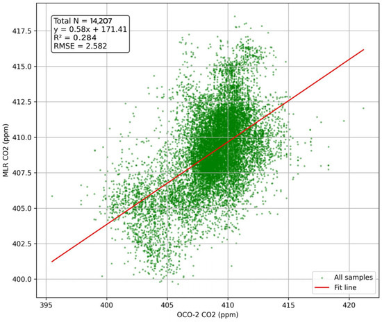
Figure 6.
Scatter plot between the original OCO-2 and reconstructed data.
As shown in Figure 6, there is an underestimation phenomenon in the low-value area, whereas there is an overestimation phenomenon in the high-value area. However, from the mean bias in Table 7, it is only larger in January, February, and December and relatively small in other months. These months represent the winter season in the Huai River Basin, where increased human activities such as heating combined with weakened carbon sink by vegetation have led to a significant rise in atmospheric concentrations. Both the error standard deviation and root mean square error were relatively small. The above results indicate that the model estimation is distributed around the mean, with a low degree of dispersion, stable data, and low volatility.
Table 7.
Accuracy verification results.
In relevant research, ref. [5] used an extreme random tree (ERT) model based on OCO-2 and environmental factors to obtain reconstructed atmospheric data (0.01° and 8-day resolution) at the global scale. The accuracy of the ERT model for the validation of the ground stations of the global continental-scale atmospheric reconstruction was assessed. The RMSE at all stations ranged from 0.9 to 3.12. Ref. [10] used a regression model with variables including GOSAT data, temperature, vegetation cover, and productivity from MODIS products to assess concentrations on a global scale. The model was verified using the GOSAT concentration as the true value. The results showed that the accuracy throughout the world is between −2.56 and 3.14 ppm. [11] used artificial neural networks to assess the spatial distribution of atmospheric concentrations over Iran during the growing season (April−September) in 2015. The modeling data included OCO-2 data and eight environmental variables. The final ANN model with the highest performance (R2) and lowest error (RMSE) for each month was selected. The range of RMSE was from 1.11 to 1.39.
Therefore, the values of the R2 and RMSE indices in this study indicate the good performance of the multiple regression model for monthly models.
3.4.3. Assessment of Spatial Pattern
Using the local variance suggested by Li et al. [24], we evaluated the ability of the reconstruction data to maintain spatial patterns at the fine scale. Local variance is a scene texture statistic that characterizes the relationship between the spatial resolution and objects in the scene [25,26]. Therefore, local variance can express the pattern information in the scene and can be used to describe the information richness of the reconstruction data. A high local variance indicates that the data have a large variability and fine patterns. The larger the local variance is, the finer the spatial pattern lies in reconstructed images [24]. The local variance is defined as Equation (3).
where is the local variance, denotes the ith pixel in the jth window, denotes the mean value of the jth window, n denotes the number of valid pixels in a moving window, and N denotes the number of windows.
We chose a 7 × 6 window and calculated the local variance. Figure 7, Table 8 and Table 9 present the monthly local variances in the reconstructed and original OCO-2 .
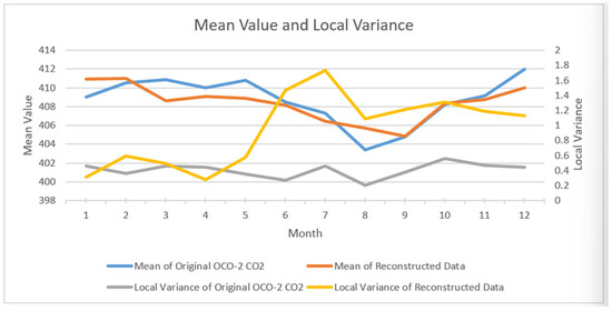
Figure 7.
Comparison of mean and local variance between reconstructed data and OCO-2 .
Table 8.
Mean value and local variance of the original OCO-2 data.
Table 9.
Mean value and local variance of the reconstructed data.
From Figure 6, Table 8 and Table 9, we can see that the monthly mean values of the reconstructed data are similar to those of the original OCO-2 data, showing strong consistency. The local variance in the reconstructed data was significantly higher than that of the original OCO-2 data, indicating that the reconstructed data contained richer detailed information and maintained the spatial pattern well at a fine scale.
3.4.4. Uncertainty Analysis
In this study, we proposed a regression framework with multiple environmental variables for retrieval in the provinces of the Huai River Basin by optimizing the selection of the input features. The results of the retrieved accuracy and reconstructed data proved our method to be high-precision and credible in the study area. However, this study has some uncertainties and limitations. First, because the model parameters were trained using the samples in the provinces of the Huai River Basin, the retrieval accuracy may decrease with the absence of land cover features if the trained model is directly applied to other study areas. However, the proposed framework—including the selection of models, the strategy of model construction, and feature optimization—remains effective for obtaining spatially completed in other study areas. The corresponding study area data can be used to retrain and refresh the model using the same framework. Second, further opportunities are available to consider land cover, quadratic polynomial simulation, and machine learning in future research. In this study, the land cover factor was not considered because if partitioned by land cover type, the number of effective OCO-2 data in partial land cover types was too small to be sufficient for modeling. In the next stage of this research, we will expand the study area and adopt machine learning and multiple regression analysis methods for zonal modeling based on land cover type. A larger study area and in situ measurements will be considered and collected to optimize the model, further improving its stability and applicability in different areas.
4. Conclusions
In this study, we constructed a multiple regression model based on the OCO-2 concentration products and multiple environmental variables, namely LAI, FVC, NPP, T, U, ET, and RH, to reconstruct the spatially complete monthly concentration data with fine resolution in the provinces in Huai River Basin in 2018. Among the multiple environmental variables, LAI, FVC, T, U, ET, NPP, and RH were strongly correlated with the concentration, whereas V was weakly correlated. These enhanced data better reflect the spatiotemporal patterns of in the study region. The proportion of valid pixels increased from less than 1% to over 90%, achieving full coverage of valid pixels in the study region. The reconstructed concentration data of the Huai River Basin have better spatial completeness. In addition to the advantage of spatial coverage, it can be seen from the comparison results of local variances that the local variance in the reconstructed dataset is significantly higher than that of the original data, indicating that the reconstructed dataset has more local detailed information.
The reconstructed atmospheric concentration showed an increasing trend from summer (June, July, and August) to winter (November, December, and January). Based on the proportion of valid pixels, local variance, and reference data, the spatial integrity, accuracy, and spatial structure of the reconstructed dataset were evaluated. The results show the value of using satellite-driven observations by extending discrete satellite observation of atmospheric concentrations to spatiotemporally continuous datasets. The regional atmospheric concentration map produced in this study can serve as a baseline map for studying regional climate change and the carbon cycle in terrestrial ecosystems. Future work will focus on using machine learning, artificial intelligence, and multisource remote sensing data to estimate a spatiotemporal complete concentration dataset with a high spatiotemporal resolution.
Author Contributions
Conceptualization, Y.Z. (Yuxin Zhu); Methodology, Y.Z. (Ying Zhang); Validation, L.Z.; Writing—review & editing, J.Z. All authors have read and agreed to the published version of the manuscript.
Funding
This research was funded by the Innovation and entrepreneurship training program for college students of Jiangsu Province (NO. 202210323050Y) and the Natural Science Foundation of China (No. 41271347).
Institutional Review Board Statement
Not applicable.
Informed Consent Statement
Informed consent was obtained from all subjects involved in the study.
Data Availability Statement
The data used in this paper can be obtained by sending an email to the first author.
Acknowledgments
This work was supported by the Innovation and entrepreneurship training program for college students of Jiangsu Province (202210323050Y) and the Natural Science Foundation of China (No. 41271347). We would like to express our sincere gratitude to the people who provided excellent comments and valuable suggestions in the preparation of this manuscript.
Conflicts of Interest
The authors declare no conflict of interest.
References
- Brethomé, F.M.; Williams, N.J.; Seipp, C.A.; Kidder, M.K.; Custelcean, R. Direct air capture of CO2 via aqueous-phase absorption and crystalline-phase release using concentrated solar power. Nat. Energy 2018, 3, 553–559. [Google Scholar] [CrossRef]
- World Meteorological Organization. Climate Change Indicators Reached Record Levels in 2023; World Meteorological Organization: Geneva, Switzerland, 2024. [Google Scholar]
- Bai, Y.; Lu, N.; Li, S. Background, challenges, opportunities and implementation paths of the dual carbon goals. China Econ. Rev. 2021, 5, 10–13. [Google Scholar]
- Chiba, T.; Haga, Y.; Inoue, M.; Kiguchi, O.; Nagayoshi, T.; Madokoro, H.; Morino, I. Measuring Regional Atmospheric CO2 Concentrations in the Lower Troposphere with a Non-Dispersive Infrared Analyzer Mounted on a UAV, Ogata Village, Akita, Japan. Atmosphere 2019, 10, 487. [Google Scholar] [CrossRef]
- Li, J.; Jia, K.; Wei, X.; Xia, M.; Chen, Z.; Yao, Y.; Zhang, X.; Jiang, H.; Yuan, B.; Tao, G.; et al. High-spatiotemporal resolution mapping of spatiotemporally continuous atmospheric CO2 concentrations over the global continent. Int. J. Appl. Earth Obs. Geoinf. 2022, 108, 102743. [Google Scholar] [CrossRef]
- Hu, K.; Liu, Z.; Shao, P.; Ma, K.; Xu, Y.; Wang, S.; Wang, Y.; Wang, H.; Di, L.; Xia, M. A Review of Satellite-Based CO2 Data Reconstruction Studies: Methodologies, Challenges, and Advances. Remote Sens. 2024, 16, 3818. [Google Scholar] [CrossRef]
- Tomosada, M.; Kanefuji, K.; Matsumoto, Y.; Tsubaki, H. A prediction method of the global distribution map of CO2 column abundance retrieved from GOSAT observation derived from ordinary Kriging. In Proceedings of the ICCAS-SICE, Fukuoka, Japan, 18–21 August 2009; pp. 4869–4873. [Google Scholar]
- Hammerling, D.M.; Michalak, A.M.; Kawa, S.R. Mapping of CO2 at high spatiotemporal resolution using satellite observations: Global distributions from OCO-2. J. Geophys. Res. Atmos. 2012, 117, 10. [Google Scholar] [CrossRef]
- Hammerling, D.M.; Michalak, A.M.; O’Dell, C.; Kawa, S.R. Global CO2 distributions over land from the Greenhouse Gases Observing Satellite (GOSAT). Geophys. Res. Lett. 2012, 39, L08804. [Google Scholar] [CrossRef]
- Guo, M.; Wang, X.; Li, J.; Yi, K.; Zhong, G.; Tani, H. Assessment of Global Carbon Dioxide Concentration Using MODIS and GOSAT Data. Sensors 2012, 12, 16368–16389. [Google Scholar] [CrossRef]
- Siabi, Z.; Falahatkar, S.; Alavi, S.J. Spatial distribution of XCO2 using OCO-2 data in growing seasons. J. Environ. Manag. 2019, 244, 110–118. [Google Scholar] [CrossRef]
- Zhang, L.; Zhao, M.; Zhao, N.; Yue, T. Modeling the Spatial Distribution of XCO2 with High Accuracy Based on OCO-2’s Observations. J. Geo-Inf. Sci. 2018, 20, 1316–1326. [Google Scholar]
- Jing, Y.; Shi, J.; Wang, T. Toward accurate XCO2 level 2 measurements by combining different CO2 retrievals from gosat and sciamachy. In Proceedings of the International Workshop on Earth Observation & Remote Sensing Applications, Changsha, China, 11–14 June 2014; p. 5. [Google Scholar]
- Wang, T.; Shi, J.; Jing, Y.; Zhao, T.; Ji, D.; Xiong, C. Combining XCO2 Measurements Derived from SCIAMACHY and GOSAT for Potentially Generating Global CO2 Maps with High Spatiotemporal Resolution. PLoS ONE 2014, 9, e0148152. [Google Scholar] [CrossRef]
- Wang, J.; Liu, Y.; Yang, D. Exploring the distribution of carbon sinks in my country: Starting from atmospheric CO2 detection. Sci. Bull. 2021, 66, 709–710. [Google Scholar] [CrossRef]
- Guo, M.; Xu, J.; Wang, X.; He, H.; Li, J.; Wu, L. Estimating CO2 concentration during the growing season from MODIS and GOSAT in East Asia. Int. J. Remote Sens. 2015, 36, 4363–4383. [Google Scholar] [CrossRef]
- Lotrecchiano, N.; Montano, L.; Bonapace, I.M.; Giancarlo, T.; Trucillo, P.; Sofia, D. Comparison Process of Blood Heavy Metals Absorption Linked to Measured Air Quality Data in Areas with High and Low Environmental Impact. Processes 2022, 10, 1409. [Google Scholar] [CrossRef]
- Liang, A.; Gong, W.; Han, G.; Xiang, C. Comparison of Satellite-Observed XCO2 from GOSAT, OCO-2, and Ground-Based TCCON. Remote Sens. 2017, 9, 1033. [Google Scholar] [CrossRef]
- Crisp, D.; Atlas, R.M.; Breon, F.-M.; Brown, L.R.; Burrows, J.P.; Ciais, P.; Connor, B.J.; Doney, S.C.; Fung, I.Y.; Jacob, D.J.; et al. The Orbiting Carbon Observatory (OCO) mission. Adv. Space Res. 2004, 34, 700–709. [Google Scholar] [CrossRef]
- Hakkarainen, J.; Ialongo, I.; Tamminen, J. Direct space-based observations of anthropogenic CO2 emission areas from OCO-2. Geophys. Res. Lett. 2016, 43, 11,400–11,406. [Google Scholar] [CrossRef]
- Liu, Q.; Wu, S.; Lei, Y.; Li, S.; Li, L. Exploring spatial characteristics of city-level CO2 emissions in China and their influencing factors from global and local perspectives. Sci. Total Environ. 2021, 754, 142206. [Google Scholar] [CrossRef] [PubMed]
- Yu, H.; Su, Z.; Zhu, P.; Chen, Y.; Yang, Q.; Zhao, Z. Relationship between Cd contents in rice or wheat and soil: Insight from a simulation study. Geosci. Front. 2021, 28, 438–445. [Google Scholar] [CrossRef]
- Chen, Y.; Lv, P.; Cao, M.; Xia, Z.; Ma, F.; Yu, J. Microclimate characteristics of Tengger Desert lakes and its response to climate change. J. Desert Res. 2024, 44, 231–238. [Google Scholar]
- Li, A.; Bo, Y.; Zhu, Y.; Guo, P.; Bi, J.; He, Y. Blending multi-resolution satellite sea surface temperature (SST) products using Bayesian maximum entropy method. Remote Sens. Environ. 2013, 135, 52–63. [Google Scholar] [CrossRef]
- Coops, N.; Culvenor, D. Utilizing local variance of simulated high spatial resolution imagery to predict spatial pattern of forest stands. Remote Sens. Environ. 2000, 71, 248–260. [Google Scholar] [CrossRef]
- Woodcock, C.E.; Strahler, A.H. The factor of scale in remote sensing. Remote Sens. Environ. 1987, 21, 311–332. [Google Scholar] [CrossRef]
Disclaimer/Publisher’s Note: The statements, opinions and data contained in all publications are solely those of the individual author(s) and contributor(s) and not of MDPI and/or the editor(s). MDPI and/or the editor(s) disclaim responsibility for any injury to people or property resulting from any ideas, methods, instructions or products referred to in the content. |
© 2025 by the authors. Licensee MDPI, Basel, Switzerland. This article is an open access article distributed under the terms and conditions of the Creative Commons Attribution (CC BY) license (https://creativecommons.org/licenses/by/4.0/).