Random Forest-Based Retrieval of XCO₂ Concentration from Satellite-Borne Shortwave Infrared Hyperspectral

Abstract

As carbon dioxide (CO₂) concentrations continue to rise, climate change, characterized by global warming, presents a significant challenge to global sustainable development. Currently, most global shortwave infrared CO₂ retrievals rely on fully physical retrieval algorithms, for which complex calculations are necessary. This paper proposes a method to predict the concentration of column-averaged CO₂ (XCO₂) from shortwave infrared hyperspectral satellite data, using machine learning to avoid the iterative computations of the physical method. The training dataset is constructed using the Orbiting Carbon Observatory-2 (OCO-2) spectral data, XCO₂ retrievals from OCO-2, surface albedo data, and aerosol optical depth (AOD) measurements for 2019. This study employed a variety of machine learning algorithms, including Random Forest, XGBoost, and LightGBM, for the analysis. The results showed that Random Forest outperforms the other models, achieving a correlation of 0.933 with satellite products, a mean absolute error (MAE) of 0.713 ppm, and a root mean square error (RMSE) of 1.147 ppm. This model was then applied to retrieve CO₂ column concentrations for 2020. The results showed a correlation of 0.760 with Total Carbon Column Observing Network (TCCON) measurements, which is higher than the correlation of 0.739 with satellite product data, verifying the effectiveness of the retrieval method.

1. Introduction

As the principal greenhouse gas, carbon dioxide (CO₂) is a key driver of global warming and climate change. Since the Industrial Revolution, atmospheric CO₂ concentrations have been rising and are currently approximately 30% higher than pre-industrial levels, with a continued upward trend [1]. The increase in CO₂ concentrations is a key driver of global warming, making its global monitoring essential for understanding the mechanisms and trends of climate change. As extreme weather events and ecological degradation intensify due to global warming, the international community has prioritized addressing this challenge through market-based mechanisms, such as carbon trading and carbon tariffs, to mitigate greenhouse gas emissions [2]. The Intergovernmental Panel on Climate Change (IPCC) explicitly stated in its Fifth Assessment Report that greenhouse gas emissions have been the primary cause of global warming since the mid-20th century. Therefore, accurately monitoring changes in atmospheric CO₂ concentrations is essential for climate prediction and the development of mitigation strategies.

Traditional ground-based measurement methods offer high precision and reliability; however, their limited spatial coverage makes it difficult to achieve global, real-time monitoring. In contrast, satellite remote sensing technology provides global coverage, continuous monitoring, and high sampling frequency, offering substantial support for the global monitoring of atmospheric CO₂. However, during this retrieval process, non-CO₂ signal factors (e.g., aerosols) have a significant impact on the retrieval results. Therefore, improving the accuracy of satellite remote sensing retrievals of CO₂ concentrations and reducing uncertainties in these measurements remain as current technical challenges that need to be addressed [3].

In recent years, atmospheric remote sensing satellite monitoring platforms have advanced rapidly, with several satellites dedicated to observing atmospheric and greenhouse gases worldwide. Examples include Japan’s Greenhouse Gases Observing Satellite (GOSAT); the United States’ Orbiting Carbon Observatory-2 (OCO-2); and China’s TanSat, Fengyun-3D (FY-3D), and GaoFen-5 (GF-5). Due to the relatively low concentration of CO₂ and its gradient compared to background values, it is essential to control the error in the average dry air mixing ratio within 1% across the global atmosphere to effectively reduce uncertainty in climate research [4,5,6,7]. However, factors such as complex atmospheric conditions, surface features, vegetation cover, temperature and humidity levels, and instrument performance can all impact the accuracy of satellite observations [8,9,10,11]. Therefore, achieving high-precision CO₂ concentration retrieval still faces many challenges.

Currently, existing shortwave infrared CO₂ observation data typically use a full-physics retrieval algorithm. This method requires simulating the entire optical path, and the calculation process of the radiative transfer equation is both complex and time-consuming [12,13]. Moreover, due to the complex effects of aerosols, water vapor, and surface reflectance on shortwave infrared radiation, existing physical retrieval models are highly dependent on input parameters, which themselves carry significant uncertainties [14,15].

To further improve the accuracy of CO₂ column concentration retrievals, machine learning techniques are increasingly being integrated into the retrieval process and have demonstrated promising application potential [16,17]. Currently, there is considerable research on using machine learning models for CO₂ retrieval and prediction. For instance, Zhao et al. [18] developed a simplified line-by-line (LBL) radiative transfer model to simulate the weak absorption band of carbon dioxide at 1.6 µm. By using the two-step machine learning model, the atmospheric spectral optical thickness can be retrieved first, and then the CO₂ column density is retrieved from the optical thickness spectrum later. Through a two-step machine learning method, it finally outputs the retrieved XCO₂, with an MAE of 0.09 ppm and a root mean square error (RMSE) of 3.13 ppm compared to GOSAT products. Xie et al. [19] proposed a novel approach based on neural network (NN) models to tackle the nonlinear retrieval problems associated with XCO₂ retrievals. The study employs a data-driven supervised learning method and explores two distinct training strategies. The error compared to OCO-2 products is 1.8 ppm, and the error compared to ground stations is approximately 0.45%. He et al. [20] employed OCO-2 XCO₂ data, Carbon Tracker XCO₂ data, and multivariate geographic data to build a model training dataset, which was then combined with various machine learning models, including Random Forest, Extreme Random Forest, et al. The results indicated that the Random Forest model presented the best performance, with a cross-validation R² of 0.878 and RMSE of 1.123 ppm. Gong et al. [21] proposed a method to predict the concentration of column-averaged CO₂ from thermal infrared satellite data using ensemble learning to avoid the iterative computations of radiative transfer models; the deviation of XCO₂ predictions of 12 TCCON sites in 2019 was within ±1 ppm.

While these studies using machine learning methods have achieved some success in retrieving CO₂ concentrations, the existing models still have certain limitations. Firstly, existing machine learning models show considerable variation in their performance for CO₂ retrievals, often resulting in large errors. When the geographical distribution or climatic conditions of the dataset change, the models’ limited cross-regional adaptability leads to increased prediction errors. Subsequently, while radiative transfer models used to simulate observed spectra typically assume relatively stable atmospheric conditions, in practical applications, the dynamic nature of the atmosphere can introduce substantial prediction errors [22,23]. Finally, contemporary machine learning approaches predominantly depend on high-quality inputs, including radiative transfer simulation data, meteorological parameters, and a priori knowledge [24]. Nevertheless, inherent uncertainties in these input data sources can directly compromise retrieval accuracy. Therefore, this study studies the applicability of OCO-2 L1b radiances and L2 products to address these issues. This study aims to obtain the spatiotemporal distribution of XCO₂ by using OCO-2 satellite data and other features through the Random Forest model, and evaluate its retrieval accuracy and influencing factors. Concurrently, it hopes that through the analysis of the retrieval results, it will provide strong support for understanding the global changes in CO₂ concentration and provide a reference for future improvements in retrieval methods.

2. Materials and Methods

2.1. Data Sources and Processing

2.1.1. OCO-2 Satellite Data

The Orbiting Carbon Observatory-2 (OCO-2) was successfully launched in July 2014, becoming the second dedicated carbon satellite globally. Its primary objective is to obtain space-based global measurements of atmospheric CO₂. With its high precision, resolution, and coverage, OCO-2 is capable of characterizing sources and sinks (fluxes) on a regional scale (≥1000 km) and quantifying CO₂ variations over seasonal cycles [25]. The L1 data products currently available on the official OCO-2 website span from 6 September 2014 to 2 April 2024. For this study, we selected the complete L1b data from 2019 [26]. The data have a spatial resolution of 2.25 km by 1.29 km and a 16-day revisit cycle, and the chosen data version is OCO2_L1B_Science_11r [27]. The fields extracted from the OCO-2 satellite observation data include latitude, longitude, solar zenith angle, observation zenith angle, solar azimuth angle, observation azimuth angle, as well as 9 high-sensitivity and 9 low-sensitivity wavelengths. To retrieve the carbon dioxide column concentration, this study uses the XCO₂ from the OCO-2 L2 product as the target variable, combining it with the features extracted from the L1 data to construct the dataset.

2.1.2. MODIS MOD04 and MCD43A3 Data

The aerosol data utilized in this study are from MODIS (Moderate-resolution Imaging Spectroradiometer) C6 aerosol product MOD04, covering the period from 2019 to 2020, and obtained from the official NASA website [28]. As a next-generation optical remote sensing instrument, MODIS provides a wide spectral range and high spatial and spectral resolution, featuring 36 spectral channels covering wavelengths from the visible to the thermal infrared [29]. The first two channels correspond to red and near-infrared wavelengths with a spatial resolution of 250 m, while channels 3 to 7 cover visible and mid-infrared wavelengths with a resolution of 500 m. Channels 8 through 36 have a resolution of 1 km. MODIS is characterized by its spectral integration capabilities and broad monitoring range, which enable it to provide comprehensive surface information [30]. The MOD04 dataset is encapsulated, and the “Corrected_Optical_Depth_Land” dataset is selected for this study, with the spatial resolution of 3 km. The dataset is then cropped and stitched according to the study area, and the mean synthesis method is applied to calculate the daily average.

The MODIS MCD43A3 dataset is a global land surface albedo product provided by NASA’s Earth Observing System (EOS) [31]. It is derived from data collected by the MODIS sensors on board the Terra and Aqua satellites, and is specifically designed to study global climate and ecosystem changes [32]. The MCD43A3 dataset provides daily albedo observations, updated every 8 days, and incorporates 16-day reflectance data to enhance data quality and coverage. It includes albedo measurements for MODIS Bands 1–7, as well as data for visible, near-infrared, and shortwave wavelengths. The dataset contains two primary albedo products: black-sky albedo and white-sky albedo, which represent total reflectance in all directions at local solar noon. The “Albedo_WSA_shortwave” dataset is selected for this study [33,34], with the spatial resolution of 500 m.

2.1.3. TCCON XCO₂ Data

Figure 1 shows the site map of the Total Carbon Column Observing Network (TCCON), an international initiative dedicated to ground-based measurements of atmospheric greenhouse gases [35]. Each TCCON site performs solar infrared spectral observations using ground-based Fourier Transform Infrared (FTIR) spectrometers, following standardized protocols. By applying a unified retrieval technique to the observed data, TCCON provides precise retrieval of various greenhouse gases, including CO₂, CH₄, N₂O, CO, HF, H₂O, HDO, and others. The network delivers real-time, continuous, and accurate column concentration measurements of these greenhouse gases on a global scale [36]. TCCON observations serve as reference standards for improving satellite algorithms and validating models, making them a critical dataset for CO₂ retrieval research. This study uses data from the Xianghe and Hefei sites, spanning from 2019 to 2021, to validate the retrieval results. The research on carbon dioxide retrieval holds significant importance for China. The Xianghe and Hefei sites are located in different geographical regions of China, representing typical climatic and atmospheric conditions of the eastern and central parts of the country, respectively. These two sites have been widely used in several related studies.

2.1.4. Data Preprocessing

For the issue of missing values during data matching, a spatial interpolation method was employed. Specifically, for each missing data point, a 3 × 3 pixel window centered on it was used to extract valid observed values, and the average of these values was calculated as the imputed value. If all pixels within the window were invalid (i.e., the average value was 0), the data point was considered invalid and removed from the dataset. This approach ensured data continuity while minimizing the impact of missing values on the retrieval results.

Since each TCCON station conducts continuous daily observations, resulting in multiple observed values, and outliers may exist in the data, it is necessary to first remove these outliers. The specific steps are as follows: For the daily observation data of each station, calculate its mean ($ӯ$) and standard deviation (σ). The range of normal values is defined as:

$$ӯ-3\mathsf{\sigma }\le \mathrm{y}\le ӯ+3\mathsf{\sigma },$$

(1)

where y is a single observed value, $ӯ$ is the mean of the daily observed data, and σ is the standard deviation of the daily data. All outliers outside the ±3σ range are removed, and the mean of the multiple observed values for each station per day is recalculated as the representative value for that station on that day. This method effectively eliminates the interference of outliers on data analysis, ensuring the reliability and accuracy of the data.

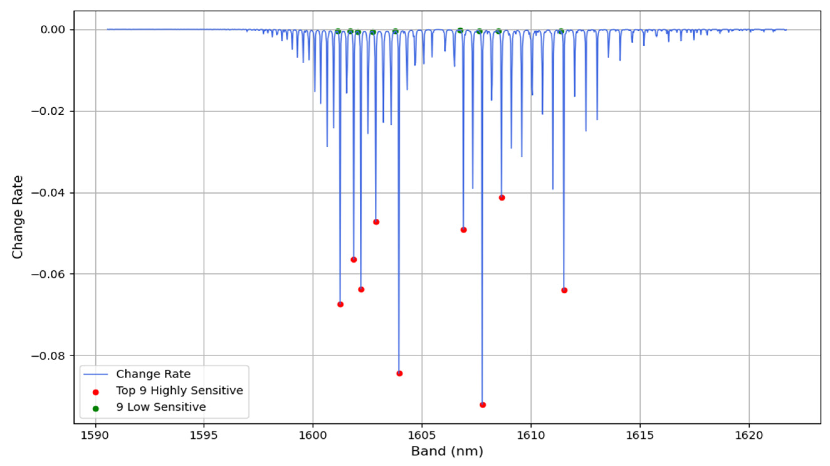
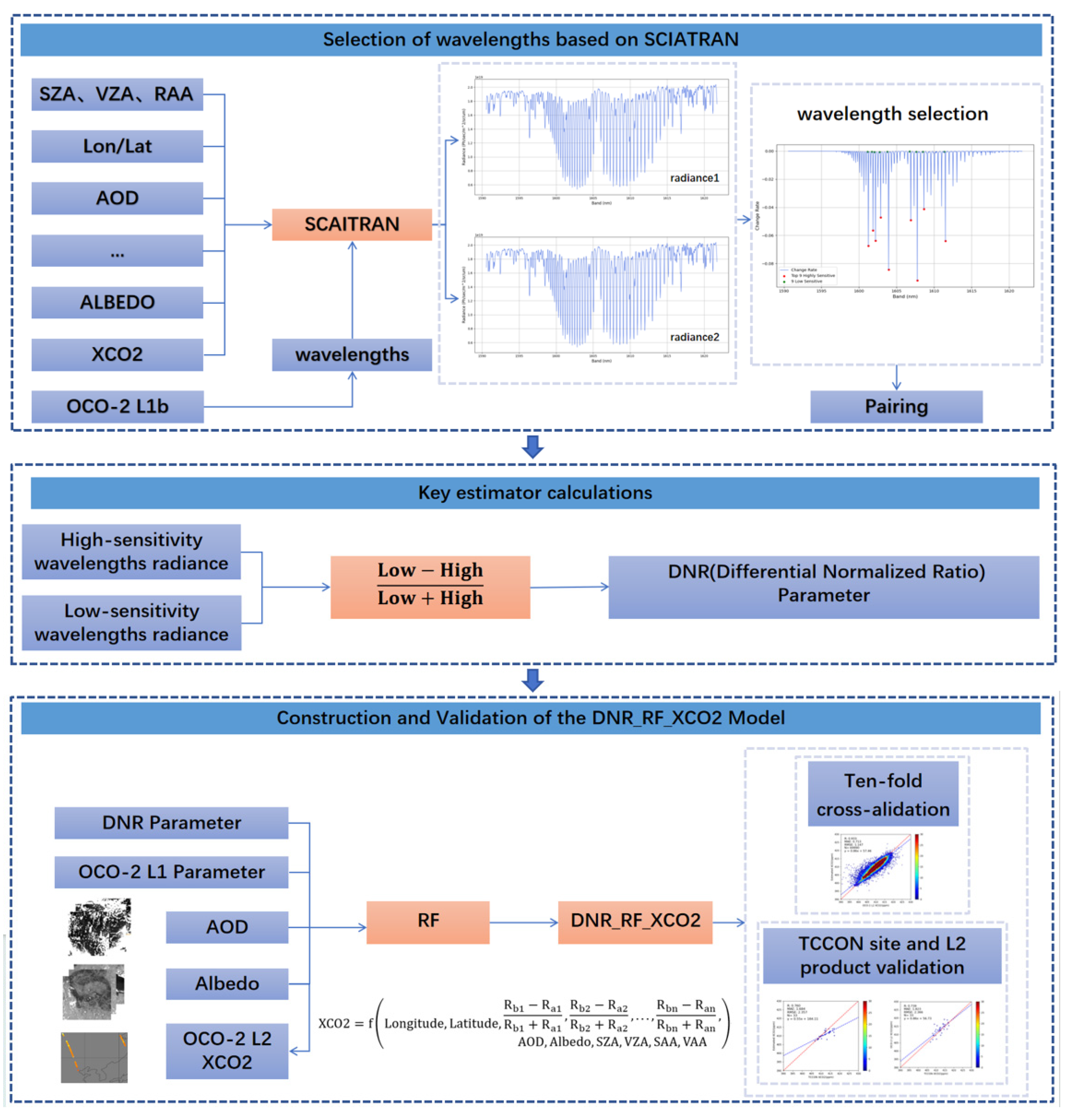
2.1.5. Retrieval Wavelength Selection

The choice of wavelength significantly impacts the accuracy and reliability of retrieval results. Since different wavelengths exhibit varying absorption characteristics for target gases or surface features, selecting the appropriate wavelength is a critical step in enhancing model accuracy [37]. This study employs the SCIATRAN radiative transfer model to perform a sensitivity analysis, identifying wavelengths with high and low sensitivity [38]. By incorporating the Differential Normalized Ratio (DNR) method, the wavelength selection process is optimized, thereby improving the stability and accuracy of the retrieval model.

Sensitivity analysis typically involves single-factor sensitivity analysis, which assumes that the model parameters are independent within a specified range. This approach is used when multiple parameters simultaneously influence the model [39]. In this analysis, only one parameter of interest is varied at a time, while all other parameters remain constant. This approach allows for an assessment of how changes in the selected parameter influence the simulation results.

As shown in Figure 2, based on the sensitivity analysis, nine highly sensitive bands around the 1.6 µm wavelength are selected. The 1.6 µm absorption band is largely unaffected by water vapor, ozone, and other atmospheric constituents, making it relatively ‘clean’ compared to other wavelengths. Furthermore, the absorption intensity at this wavelength is moderate, thus avoiding absorption saturation [40]. Since CO₂ is primarily concentrated near Earth’s surface and the 1.6 µm wavelength is highly sensitive to near-surface CO₂ concentrations, the 1.6 µm absorption band is the most suitable for this simulation. To select the most sensitive wavelengths, this study incorporates various parameters in the SCIATRAN radiative transfer model, including observation geometry, aerosol properties, surface albedo, and different CO₂ concentrations. By comparing the rate of change in simulated radiance under these varying parameters, the nine wavelengths with the largest variation were identified: 1607.77, 1603.947, 1601.251, 1611.516, 1602.201, 1601.875, 1606.907, 1602.884, and 1608.655 (nm). These wavelengths are selected as the highly sensitive wavelengths for this study.

After identifying the highly sensitive wavelengths, the next step is to select appropriate insensitive wavelengths using variation rate analysis. Near the peak of the highly sensitive wavelength, the first derivative of the spectral absorption curve is calculated, and the wavelength with the smallest variation rate is chosen as the insensitive wavelength. These wavelengths are less influenced by CO₂ absorption and better reflect the characteristics of background radiation or non-target absorptions. Finally, for each highly sensitive wavelength, nine insensitive wavelengths with the smallest variation rates, including 1607.555, 1603.786, 1601.415, 1611.837, 1602.364, 1601.744, 1606.721, 1602.722, and 1608.867 (nm), are selected to provide a sufficient background reference. This strategy of pairing sensitive and insensitive wavelengths enhances the robustness of the retrieval algorithm and improves its ability to correct for interference factors.

2.2. Model Dataset Construction

After identifying the highly sensitive and low-sensitive wavelengths, the Differential Normalized Ratio (DNR) method is applied to extract feature values (denoted as band1 to band9). This method calculates the ratio of the difference in radiance between the sensitive and insensitive wavelengths to the sum of their radiances. This approach helps to mitigate the effects of light source intensity and background radiation, thereby emphasizing the absorption characteristics of the target gas. Furthermore, this method effectively suppresses noise interference from non-target wavelengths, enhancing the stability and robustness of the retrieval results. Building on this, the previously identified feature values are combined with seven physical variables and two environmental variables: latitude and longitude, SZA, VZA, SAA, VAA, OCO-2 L2 product XCO₂, surface albedo (Albedo), and AOD, as listed in

Table 1. The specific features used for model training.

Data Sources	Data	Units	Spatial Resolution	Temporal Resolution
OCO-2 L1b	Radiance	Ph/s/m2/sr/um	1.29 km × 2.25 km	16 day
	Longitude	degrees
	Latitude	degrees
	Solar zenith angle (SZA)	degrees
	View zenith angle (VZA)	degrees
	Solar azimuth angle (SAA)	degrees
	View azimuth angle (VAA)	degrees
OCO-2 L2	XCO2	ppm	1.29 km × 2.25 km	16 day
MOD04_3 km	Aerosol optical depth (AOD)	-	3 km	1 day
MCD43A3	Albedo	-	500 m	1 day

. Through spatiotemporal matching of these multi-source data, a retrieval dataset is constructed.

2.3. Model Description

Random Forest is an ensemble learning algorithm that relies on decision trees, employing the Bagging method and random feature selection for model training [41]. By constructing multiple decision trees and aggregating their results through voting or averaging, Random Forest mitigates the overfitting risk associated with individual decision trees and enhances the model’s ability to generalize. Key advantages of Random Forest include its strong adaptability to nonlinear relationships, robustness for missing data, and capacity to assess feature importance [42,43,44]. The hyperparameters of the Random Forest model, such as the number of trees (n_estimators) and maximum depth (max_depth), were optimized using Bayesian optimization. This approach efficiently explores the hyperparameter space to minimize prediction error, ensuring robust model performance.

In this study, the Random Forest model was employed to retrieve the XCO₂ values from OCO-2 satellite observation data. The radiance values from 9 high-sensitivity and 9 low-sensitivity wavelengths, selected from the OCO-2 L1 data, were used to calculate spectral feature values using the Differential Normalized Ratio (DNR) method. These features were combined with additional variables, including longitude, latitude, SZA, VZA, SAA, VAA, albedo, AOD, and XCO₂ from the OCO-2 L2 products. The features were carefully matched in both time and space to ensure the accuracy and consistency of the retrieval data. The model was trained and tested using data from 2019, with a training-to-test ratio of 9:1, and its performance was evaluated through ten-fold cross-validation.

3. Results

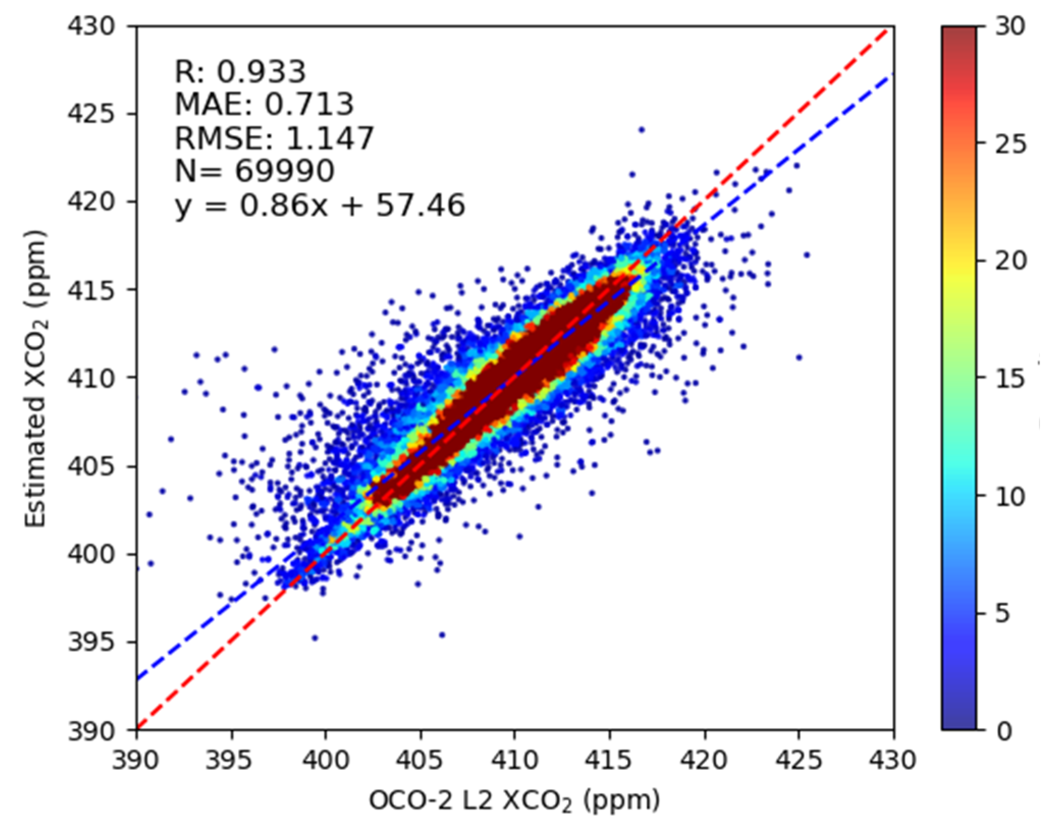
3.1. Model Accuracy Evaluation

As shown in the flowchart in Figure 3, the study used three models for prediction: Random Forest, XGBoost, and LightGBM. The dataset, consisting of 69,990 matched data points, was initially split into training and testing sets with a 9:1 ratio. During each model training phase, the data order was randomly shuffled, and the dataset was re-split to ensure that each iteration used a unique subset of data. This approach enhances the robustness of the experiment by preventing the models from being trained on identical data subsets.

As shown in

Table 2. Detailed settings of model parameters and results.

Model	n_Estimators	Max_Depth	R	MAE (ppm)	RMSE (ppm)
Random Forest	220	100	0.933	0.713	1.147
XGBoost	143	9	0.929	0.768	1.182
LightGBM	442	163	0.840	1.222	1.731

, the results show that the R values were 0.933, 0.929, and 0.840 for Random Forest, XGBoost, and LightGBM, respectively. The MAE values were 0.713, 0.768, and 1.222 (ppm), and the RMSE values were 1.147, 1.182, and 1.731 (ppm). The Random Forest model exhibited the highest R and the lowest RMSE and MAE. Considering these along with the three model evaluation metrics, Random Forest demonstrated the best performance in model validation, showing high prediction accuracy and minimal errors. Thus, the Random Forest model was ultimately chosen to estimate XCO₂. In line with its construction characteristics, the model was named DNR_RF_XCO₂, where ‘DNR’ signifies the model’s integration of dynamic and robust features for accurate CO₂ concentration estimation.

In Figure 4, ten-fold cross-validation was performed on the training data using the Random Forest model. In the sample-based ten-fold cross-validation process, the dataset is first randomly divided into 10 subsets. In each round, one subset is used as the validation set, while the model is trained on the remaining nine subsets. The main objective of this process is to ensure that all samples are included in both the training and validation phases, allowing for a comprehensive evaluation of the model’s ability to generalize. After each round of training, the model’s predictions on the validation set are compared with the actual measured XCO₂ values. This process is repeated for a total of 10 rounds, providing a robust evaluation of the model’s performance.

The results showed that the model exhibited high predictive accuracy. These indicators suggest that while the model effectively captures the underlying patterns in the data, it exhibits a low prediction error, demonstrating strong predictive capability. Moreover, the high correlation coefficient indicates the model’s strong fitting ability for the target variable, while the low MAE and RMSE values suggest that the model’s predictions are stable and reliable. These results validate the applicability of the Random Forest model in this research task, providing a solid foundation for subsequent analysis. Despite the promising performance of the Random Forest model, several potential sources of uncertainty were considered: (1) Non-CO₂ Signal Interference: Errors may arise from non-CO₂ signals, such as those caused by atmospheric conditions like cloudy or high-aerosol areas. These conditions can interfere with the accurate retrieval of CO₂ concentrations, leading to potential biases in the results. (2) Data Matching and Interpolation Errors: During data matching, missing values were addressed using a spatial interpolation method. Specifically, a 3 × 3 pixel window centered on each missing data point was used to extract valid observed values, and the average of these values was calculated as the imputed value. However, if all pixels within the window were invalid (i.e., the average value was 0), the data point was removed. While this approach ensures data continuity, it may introduce errors due to the inherent limitations of interpolation and the potential loss of valid data points. (3) Model Intrinsic Errors: The retrieval model itself may contribute to errors due to uncertainties in its assumptions, parameterizations, or simplifications. These intrinsic errors can propagate through the analysis and affect the overall accuracy of the results.

3.2. Retrieval Accuracy Evaluation

This study utilizes XCO₂ data from two TCCON stations in 2020 and 2021 to validate the retrieval results. The first station, Xianghe, is located in China at coordinates (39.8° N, 116.96° E) with an altitude of 0.036 km, while the second station, Hefei, is situated at (31.91° N, 117.17° E) with an altitude of 0.029 km [45]. Data from the OCO-2 satellite, specifically, from the orbital passes over these stations, were selected for differential normalized ratio retrieval. First, the daily average results were compared, and the correlation between the OCO-2 retrievals and the TCCON ground-based measurements was calculated. Second, a comparative analysis was performed using the daily average data alongside the OCO-2 L2 product data [46].

Figure 5a,b show the results indicate that the correlation between the OCO-2 retrievals and ground station measurements is 0.760, which is higher than the correlation between the OCO-2 L2 products and the ground stations. This suggests that the differential normalized ratio retrieval method effectively reduces the impact of systematic errors, thereby enhancing the model’s ability to capture observation signals. Furthermore, the retrieval method demonstrates greater adaptability to local climate conditions and atmospheric characteristics, resulting in more accurate CO₂ concentration estimates. This improvement in accuracy not only validates the effectiveness of the retrieval method but also highlights its potential to enhance the accuracy of existing satellite products and facilitate ground-based observation validation.

Figure 6a,b show that the DNR_RF_XCO₂ model estimates in the vicinity of the Xianghe station on 7 November 2019 are well aligned with the XCO₂ distribution from the OCO-2 L2 product. In most areas, the model estimates closely match the observed values, demonstrating the model’s strong predictive capability in this region. A similar trend is seen in Figure 6c,d, where the DNR_RF_XCO₂ estimates near the Hefei station on 12 March 2019 also align with the OCO-2 L2 XCO₂ distribution, further confirming the model’s stability and accuracy across different geographical locations. The Figure 6 scatter plots show the distribution of OCO-2 L2 XCO₂ values and DNR_RF_XCO₂ retrieval results for the Xianghe and Hefei stations, respectively.

3.3. Spatiotemporal Extension Evaluation

The retrieval of the CO₂ concentration is a complex task influenced by various factors, such as spectral characteristics, atmospheric conditions, surface reflectance, and instrument properties [47]. These factors can vary significantly across different spatiotemporal scales, making the model’s spatiotemporal transferability crucial. This study validated the spatiotemporal transferability of the model using data from 2020, and the results indicate that the model still possesses high predictive capability under different temporal and spatial conditions.

In Figure 7, the model demonstrated a correlation coefficient R of 0.776, a mean absolute error (MAE) of 2.213 ppm, and a root mean square error (RMSE) of 2.840 ppm when compared with the OCO-2 satellite L2 product in the validation dataset of 2020. This result indicates that, despite the training data being sourced from 2019, the model can still adapt to changes in atmospheric conditions, surface optical properties, and different observational geometries in 2020, showcasing its good spatiotemporal transferability. Compared to traditional products, the model’s higher correlation and lower errors further prove its advantage in capturing detailed variations. In our study, the mean bias of the retrieved XCO₂ is 1.87 ppm; this suggests that our retrieval algorithm can partially capture the global annual increase in XCO₂.

In addition, the good performance of the model in spatiotemporal migration is also due to its use of the differential normalization ratio retrieval method, which can effectively reduce the impact of systematic errors and improve the sensitivity to local climate characteristics and atmospheric vertical structure changes [48].

In summary, the retrieval model of this study not only shows high accuracy within the range of training data, but also demonstrates excellent performance in spatiotemporal transfer through validation.

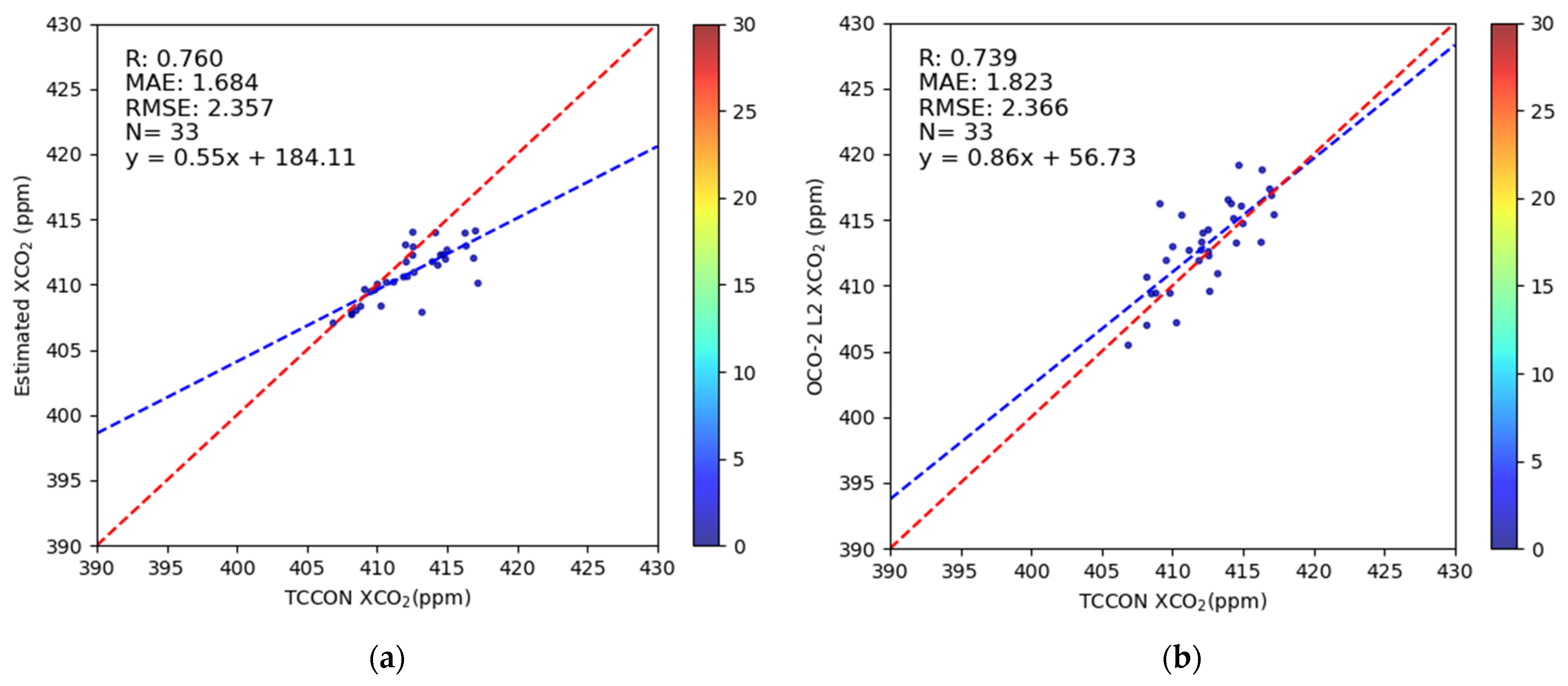
3.4. Analysis Based on TCCON Sites

In Figure 8, we analyze the correlation between the retrieval values and ground-based TCCON observations at Xianghe station and Hefei station. The correlation coefficient between the retrieved XCO₂ values and ground-based observations at Xianghe station in Figure 8a is 0.82, indicating that the retrieval value of Xianghe station has a strong linear relationship with the ground-based TCCON data, and the retrieval accuracy is high. In contrast, the correlation between Hefei station and ground-based observation in Figure 8b is 0.69, reflecting the low correlation between the retrieval value of Hefei station and ground-based TCCON data. Although the correlation of Hefei station is slightly lower, it still shows similar seasonal and interannual variation trends as ground-based TCCON data.

Several factors may contribute to the differences between retrieved XCO₂ and ground-based observations at Xianghe and Hefei stations. First, the geographical location and climatic conditions of Xianghe station may favor higher retrieval accuracy. The region where Xianghe station is located may have more stable atmospheric conditions and better temporal matching, which improves the consistency of the retrieval results with the ground-based TCCON data. The lower correlation at Hefei station may be related to the local climate variability, aerosols, surface albedo, and other factors that may affect the retrieval accuracy [36,49].

In addition, although there is a certain deviation between the retrieval value and the ground observation data—especially, the retrieval value at Hefei station is lower than the ground TCCON data—the seasonal and interannual variation trends of the two are highly consistent. This shows that although there are systematic errors, the retrieval method can still better capture the change trend of the atmospheric CO₂ concentration, indicating that the retrieval method based on satellite data has good potential and can effectively provide support for global CO₂ monitoring.

3.5. Comparison of Results from Different Parameter Models

In order to comprehensively evaluate the performance of different models in CO₂ column concentration retrieval, this study designed four feature combination models: only using high-sensitivity wavelengths (Model 1), high-sensitivity plus low-sensitivity wavelengths (Model 2), low-sensitivity to high-sensitivity wavelengths (Model 3), and low-sensitivity combined with high-sensitivity wavelengths based on the differential normalized ratio (DNR) (Model 4). Model 4, referred to as DNR_RF_XCO₂ in the previous figures, is the differential normalized ratio (DNR)-based model combining low-sensitivity and high-sensitivity wavelengths.

As shown in

Table 3. Model parameters of four different models.

Model	Model Radiance Parameters	Model Parameters
Model 1	Highly sensitive	$\mathrm{X}\mathrm{C}{\mathrm{O}}_2=\mathrm{f}\left(\begin{array}{c}\mathrm{Longitude},\mathrm{Latitude},{\mathrm{R}}_{\mathrm{a}1},{\mathrm{R}}_{\mathrm{a}2},\dots ,{\mathrm{R}}_{\mathrm{a}\mathrm{n}},\\ \mathrm{A}\mathrm{O}\mathrm{D},\mathrm{A}\mathrm{l}\mathrm{b}\mathrm{e}\mathrm{d}\mathrm{o},\mathrm{S}\mathrm{Z}\mathrm{A},\mathrm{V}\mathrm{Z}\mathrm{A},\mathrm{S}\mathrm{A}\mathrm{A},\mathrm{V}\mathrm{A}\mathrm{A}\end{array}\right)$
Model 2	Highly sensitive + Low sensitive	$\mathrm{X}\mathrm{C}{\mathrm{O}}_2=\mathrm{f}\left(\begin{array}{c}\mathrm{L}\mathrm{o}\mathrm{n}\mathrm{g}\mathrm{i}\mathrm{t}\mathrm{u}\mathrm{d}\mathrm{e},\mathrm{L}\mathrm{a}\mathrm{t}\mathrm{i}\mathrm{t}\mathrm{u}\mathrm{d}\mathrm{e},{\mathrm{R}}_{\mathrm{a}1},{\mathrm{R}}_{\mathrm{a}2},\dots ,{\mathrm{R}}_{\mathrm{a}\mathrm{n}},{\mathrm{R}}_{\mathrm{b}1},{\mathrm{R}}_{\mathrm{b}2},\dots ,{\mathrm{R}}_{\mathrm{b}\mathrm{n}},\\ \mathrm{A}\mathrm{O}\mathrm{D},\mathrm{A}\mathrm{l}\mathrm{b}\mathrm{e}\mathrm{d}\mathrm{o},\mathrm{S}\mathrm{Z}\mathrm{A},\mathrm{V}\mathrm{Z}\mathrm{A},\mathrm{S}\mathrm{A}\mathrm{A},\mathrm{V}\mathrm{A}\mathrm{A}\end{array}\right)$
Model 3	Low sensitive/Highly sensitive	$\mathrm{X}\mathrm{C}{\mathrm{O}}_2=\mathrm{f}\left(\begin{array}{c}\mathrm{L}\mathrm{o}\mathrm{n}\mathrm{g}\mathrm{i}\mathrm{t}\mathrm{u}\mathrm{d}\mathrm{e},\mathrm{L}\mathrm{a}\mathrm{t}\mathrm{i}\mathrm{t}\mathrm{u}\mathrm{d}\mathrm{e},{\displaystyle \frac{{\mathrm{R}}_{\mathrm{b}1}}{{\mathrm{R}}_{\mathrm{a}1}}},{\displaystyle \frac{{\mathrm{R}}_{\mathrm{b}2}}{{\mathrm{R}}_{\mathrm{a}2}}},\dots ,{\displaystyle \frac{{\mathrm{R}}_{\mathrm{b}\mathrm{n}}}{{\mathrm{R}}_{\mathrm{a}\mathrm{n}}}},\\ \mathrm{A}\mathrm{O}\mathrm{D},\mathrm{A}\mathrm{l}\mathrm{b}\mathrm{e}\mathrm{d}\mathrm{o},\mathrm{S}\mathrm{Z}\mathrm{A},\mathrm{V}\mathrm{Z}\mathrm{A},\mathrm{S}\mathrm{A}\mathrm{A},\mathrm{V}\mathrm{A}\mathrm{A}\end{array}\right)$
Model 4	(Low sensitive − Highly sensitive)/(Low sensitive + Highly sensitive)	$\mathrm{X}\mathrm{C}{\mathrm{O}}_2=\mathrm{f}\left(\mathrm{L}\mathrm{o}\mathrm{n}\mathrm{g}\mathrm{i}\mathrm{t}\mathrm{u}\mathrm{d}\mathrm{e},\mathrm{L}\mathrm{a}\mathrm{t}\mathrm{i}\mathrm{t}\mathrm{u}\mathrm{d}\mathrm{e},\begin{array}{c}{\displaystyle \frac{{\mathrm{R}}_{\mathrm{b}1}-{\mathrm{R}}_{\mathrm{a}1}}{{\mathrm{R}}_{\mathrm{b}1}+{\mathrm{R}}_{\mathrm{a}1}}},{\displaystyle \frac{{\mathrm{R}}_{\mathrm{b}2}-{\mathrm{R}}_{\mathrm{a}2}}{{\mathrm{R}}_{\mathrm{b}2}+{\mathrm{R}}_{\mathrm{a}2}}},\dots ,{\displaystyle \frac{{\mathrm{R}}_{\mathrm{b}\mathrm{n}}-{\mathrm{R}}_{\mathrm{a}\mathrm{n}}}{{\mathrm{R}}_{\mathrm{b}\mathrm{n}}+{\mathrm{R}}_{\mathrm{a}\mathrm{n}}}},\\ \mathrm{A}\mathrm{O}\mathrm{D},\mathrm{A}\mathrm{l}\mathrm{b}\mathrm{e}\mathrm{d}\mathrm{o},\mathrm{S}\mathrm{Z}\mathrm{A},\mathrm{V}\mathrm{Z}\mathrm{A},\mathrm{S}\mathrm{A}\mathrm{A},\mathrm{V}\mathrm{A}\mathrm{A}\end{array}\right)$

, through experimental analysis, the ten-fold cross-validation results of these four models on the 2019 data are very close, with a correlation coefficient of about 0.933, indicating that the feature extraction methods of each model have high prediction ability under static conditions. However, further testing of its spatiotemporal migration performance, i.e., using the model trained in 2019 to predict the data in 2020, shows that Model 4 performs best, with a correlation coefficient (R) of 0.776, and MAE and RMSE of 2.213 ppm and 2.840 ppm, respectively, which is better than the other three models, and the model results are shown in

Table 4. The different evaluation metrics for the model training results.

Model	Ten-Fold Cross-Validation in 2019			Retrieval Results in 2020
	R	MAE	RMSE	R	MAE	RMSE
Model 1	0.932	0.715	1.151	0.736	2.419	2.944
Model 2	0.933	0.723	1.151	0.764	2.360	2.801
Model 3	0.933	0.723	1.151	0.682	2.599	3.253
Model 4	0.933	0.713	1.147	0.776	2.213	2.840

.

In contrast, the performance of spatiotemporal transfer for other models is not satisfactory. For example, the R value of Model 1 is 0.736, and that of Model 3 is even lower at 0.682, while although the performance of Model 2 has been improved, its R value is 0.764, which is still lower than that of Model 4. In addition, the MAEs of Model 4 are the smallest among the four models, which indicates that it not only has better prediction accuracy but also has significant advantages in adaptability to spatial and temporal changes. The above results show that the feature combination based on the differential normalization ratio method can better capture the relative change characteristics between high-sensitive and low-sensitive wavelengths, and the combination with other input features (e.g., solar zenith angle, observation zenith angle) effectively improves the generalization ability of the model. Therefore, Model 4 was finally selected as the optimal model to achieve high-precision and high-robustness CO₂ column retrieval in this study.

The DNR method (Model 4) demonstrates consistent and significant improvements over other methods in both ten-fold cross-validation (2019) and retrieval results (2020). In the 2019 cross-validation, Model 4 achieved the lowest MAE (0.713) and RMSE (1.147), slightly outperforming Models 1–3 (MAE = 0.715–0.723, RMSE = 1.151). For the 2020 retrieval results, Model 4 showed more pronounced enhancements, achieving the highest correlation coefficient (R = 0.776), the lowest MAE (2.213), and a competitive RMSE (2.840) compared to Models 1–3 (R = 0.682–0.764, MAE = 2.360–2.599, RMSE = 2.801–3.253). Specifically, compared to the best baseline model (Model 2), Model 4 improved R by 1.57%, reduced MAE by 6.23%, and lowered RMSE by 1.39%. Through the DNR method, the characteristic information of carbon dioxide was highlighted, while potential interferences from aerosols and other gas species were minimized. These results demonstrate the capability of the DNR method in improving retrieval accuracy and reducing errors.

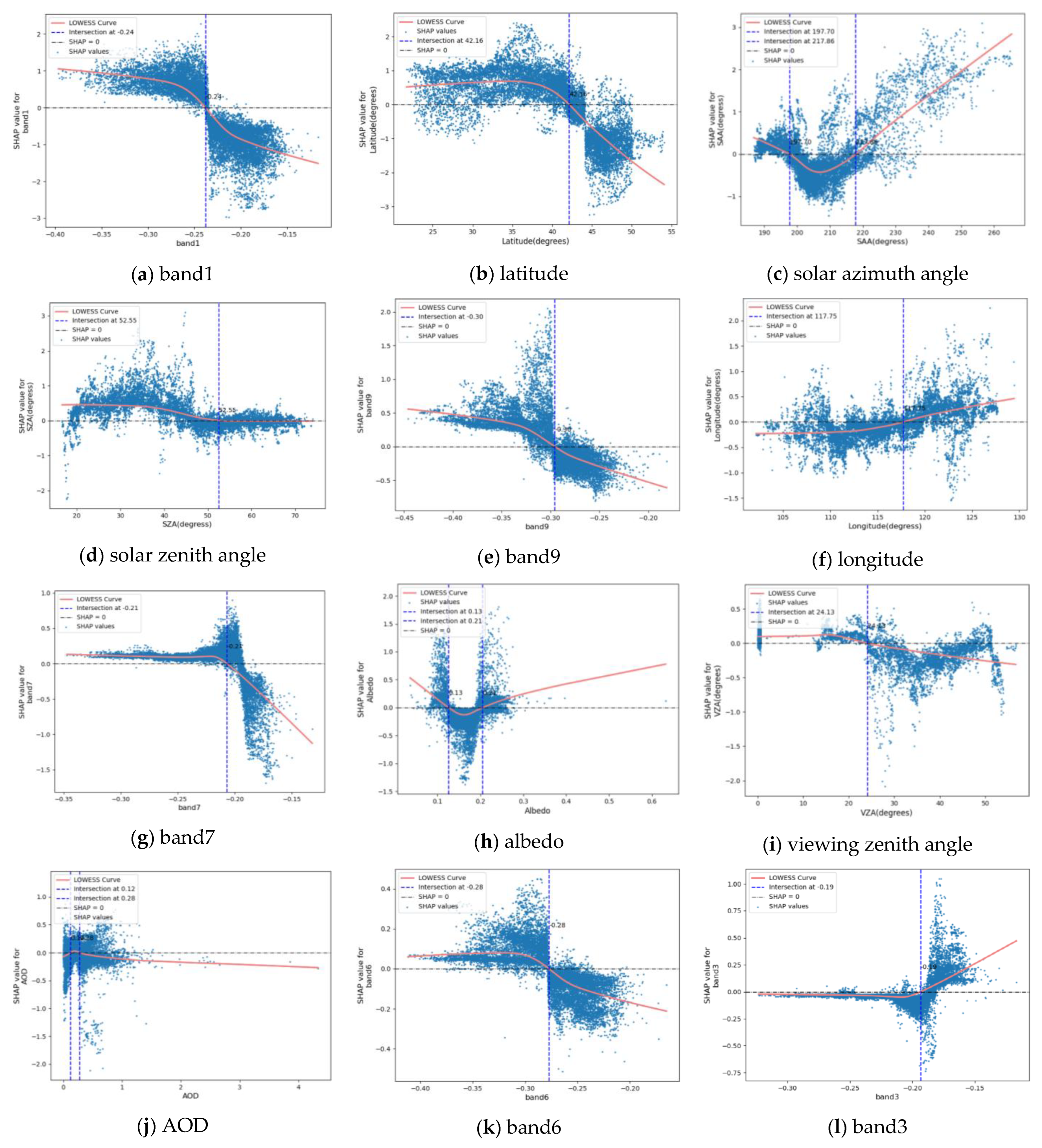
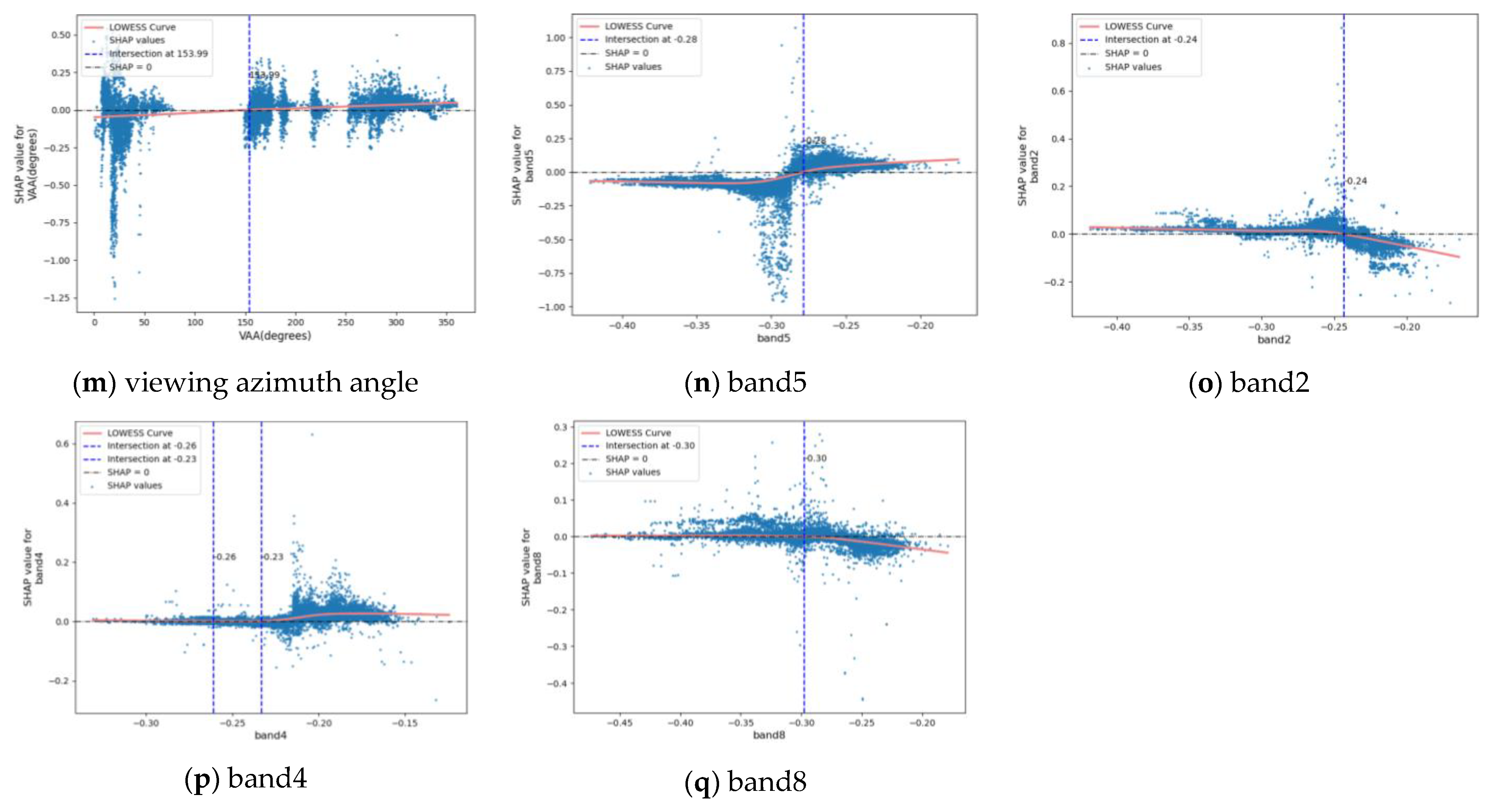
3.6. SHAP Interpretable Analysis

In this study, Shapley analysis is used to assess the impact of various factors listed in Table 1. It provides a more accurate quantitative ranking of influence by calculating feature weights from both local and global perspectives [50,51,52].

In the SHAP bar chart of Figure 9a, the wavelengths band1 and band9, Latitude, SAA, and SZA are listed as the five features that contribute the most to the model’s prediction results. This indicates that the model’s predictions primarily rely on these spectral and geometric characteristics. The high importance of wavelengths band1 and band9 might be related to the target variable being highly sensitive to the spectral absorption or scattering properties at these wavelengths, while the significance of latitude, solar azimuth angle, and solar zenith angle reflects the substantial impact of spatial distribution and lighting conditions on the target variable. The ranking of these features suggests that the model not only considers the spectral characteristics of the target variable but also fully integrates geographical and solar position parameters, achieving precise extraction of complex features from observational data.

The Figure 9b honeycomb diagram further reveals the specific contribution direction and magnitude of feature values to the prediction [52]. Among them, the high values of wavelength band1 and band9 have a negative contribution to the prediction results, while the low values have a positive contribution, indicating that the high radiance of these wavelengths may be related to lower target values, which may be caused by the enhancement of specific absorption characteristics. The distribution of latitude (Latitude) features shows that high-latitude areas contribute negatively to the target value, and low-latitude areas contribute positively to the target value, which is consistent with the natural distribution law of the target variable at different latitudes. SAA presents an opposite pattern, indicating that the larger its value, the higher the contribution to the target value, while the contribution of SZA is mainly concentrated in the middle-value range, indicating its nonlinear impact characteristics. These results collectively reflect the model’s ability to capture complex feature mechanisms and validate the rationality of data preprocessing and model construction.

The LOWESS curve (red line) in Figure 10 is a locally weighted regression curve, which is used to smooth the nonlinear trends in the data. In the graph, it represents the average impact trend of different features on the target variable. From the curve, it can be seen that as the feature values change, the SHAP values fluctuate accordingly. Through this fitted curve, different contributions of different feature intervals to model prediction can be identified. The blue dashed lines in the graph mark the intersections, respectively, representing the intersections of the SHAP value curve with y = 0. These two intersections indicate that at specific features, the SHAP value is zero, meaning that at these points, the features’ impact on the model gradually transition from negative to positive or vice versa.

Figure 10 illustrates the trends and nonlinear relationships between feature values (band1, latitude, solar azimuth angle, and others) and their corresponding SHAP values. The results reveal how each feature contributes positively or negatively to the model’s predictions within specific value ranges. For a detailed analysis of each subplot, please refer to the figure caption.

The above, through fitting curves and intersections, allows for a more intuitive understanding of the nonlinear impact of features on model prediction results. Especially, these intersections reveal the key change points of features in specific intervals for the target variable, which helps to understand how the model handles different features, and how to make more precise interpretations.

4. Discussion

The machine learning-based shortwave infrared CO₂ column concentration remote sensing retrieval method proposed in this study achieved relatively accurate CO₂ concentration prediction results, especially when compared with satellite observation data. The model successfully retrieved high-precision XCO₂ using 18 spectral channels and demonstrated a high correlation (0.933) and low error (MAE: 0.713 ppm, RMSE: 1.147 ppm), indicating that the selected wavelengths encompass core information and that the machine learning model can significantly improve the accuracy of satellite remote sensing CO₂ concentration retrieval, effectively reduce systematic errors, and enhance spatiotemporal adaptability. The retrieval results show that the changes in CO₂ concentration in space and time are significant and are affected by geographical location, climatic conditions, and atmospheric characteristics. Through the validation of data from 2020 and 2021, the adaptability of the model in different years and regions has been verified, showing high accuracy and stability. Compared with TCCON ground station data, the correlation between the model and ground stations is 0.760, further verifying the effectiveness of this method in practical applications. The influencing factors of retrieval accuracy include atmospheric conditions (such as aerosols, surface albedo, etc.) and observation geometry (such as solar zenith angle, observation zenith angle, etc.) [53]. Especially through the differential normalization ratio (DNR) method, the model effectively reduces the impact of these uncertainty factors on the retrieval results. In addition, wavelength selection plays a crucial role in improving accuracy, especially the selection of highly sensitive wavelengths, such as 1607.77 and 1603.947, which can better capture the absorption characteristics of CO₂, reduce background interference, and improve retrieval accuracy.

As climate change progresses, accurate and reliable CO₂ measurements are crucial for tracking the effectiveness of emission reduction strategies and for validating carbon cycle models. The proposed methodology offers an enhanced tool for global CO₂ monitoring, especially in remote and hard-to-reach areas where ground-based measurements are sparse.

Despite this, the accuracy of the model depends on the quality and quantity of training data. Therefore, in extreme climatic conditions or uncommon geographical areas, it may not be fully adapted, leading to increased errors [54]. Future research can focus on introducing more diverse remote sensing data and incorporating a larger variety of ground observation datasets to improve the model’s generalization capability. Enhancing feature selection and model algorithms, improving sensitivity to atmospheric interference factors, and further reducing systematic errors are essential to advancing the accuracy of CO₂ concentration retrieval. Furthermore, expanding the model’s applicability to a broader range of conditions, such as extreme weather events or unusual geographical areas, will be crucial in enhancing its utility for large-scale CO₂ monitoring and climate change research.

5. Conclusions

This paper combines OCO-2 satellite observation data, TCCON station observation data, and AOD data to propose a shortwave infrared CO₂ column concentration retrieval method based on machine learning.

(1)

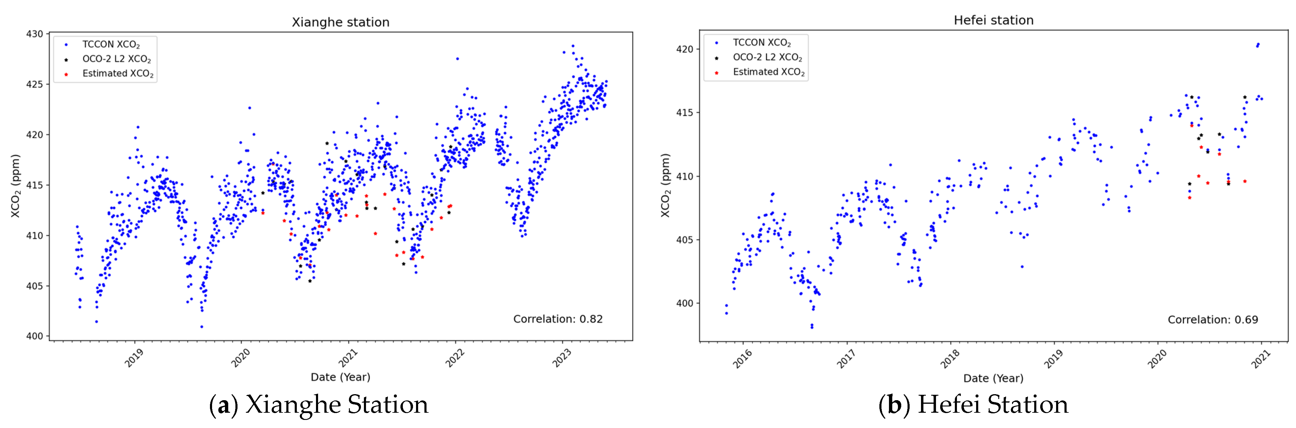
The results show that it can effectively invert the atmospheric CO₂ concentration, and the correlation with the TCCON ground station data when spatially and temporally migrated to different years is 0.760, indicating that this method has broad application prospects in improving the accuracy of CO₂ concentration monitoring.

(2)

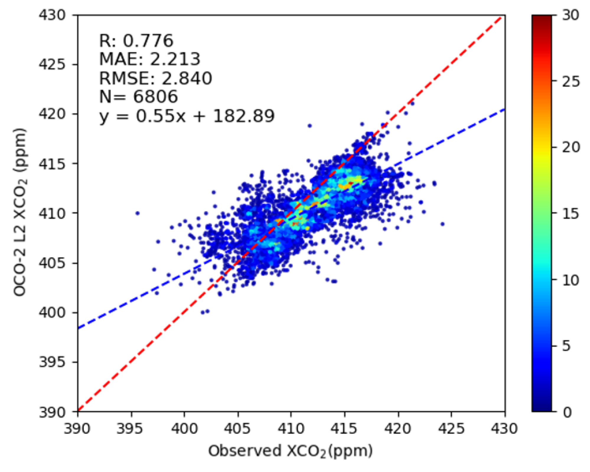
Compared with the existing OCO-2 satellite products, the retrieval method in this paper can significantly reduce systematic errors and demonstrates strong spatiotemporal adaptability, being able to accurately invert CO₂ concentrations under different time and regional conditions, verifying its stability and reliability under various environmental conditions.

(3)

Future research can further optimize the retrieval model by adding more feature variables (such as climate patterns, other satellite data) and improve machine learning algorithms to further enhance retrieval accuracy. Combining more satellite data (such as GOSAT, TanSat, etc.) and ground station data can enhance the diversity of the training set, further improving the robustness and accuracy of the model. At the same time, further improving the model’s spatiotemporal migration capability, especially its performance under extreme climatic conditions, will be a key direction for the future.

(4)

We developed an integrated approach combining OCO-2 satellite spectral data, TCCON ground-based measurements, aerosol optical depth (AOD), and surface albedo, ultimately establishing the DNR_RF_XCO₂ carbon dioxide retrieval model. The model validated its transferability over diverse regions (e.g., Xianghe and Hefei stations) and temporal scales (2019–2021), with consistent performance under varying climatic conditions (e.g., R = 0.776 in 2020). This establishes a reliable foundation for operational large-scale CO₂ monitoring and supports methodological advancements for next-generation greenhouse gas satellites.

References

1. Liu, L.; Chen, L.; Liu, Y.; Yang, D.; Zhang, X.; Lu, N.; Ju, W.; Jiang, F.; Yin, Z.; Liu, G.; et al. Satellite remote sensing for global stocktaking: Methods, progress and perspectives. J. Remote Sens. 2022, 26, 243–267. [Google Scholar] [CrossRef]
2. Liu, Y.; Wang, J.; Che, K.; Cai, Z.; Yang, D.; Wu, L. Satellite remote sensing of greenhouse gases: Progress and trends. Natl. J. Remote Sens. Bull. 2021, 25, 53–64. [Google Scholar] [CrossRef]
3. Hu, K.; Liu, Z.; Shao, P.; Ma, K.; Xu, Y.; Wang, S.; Wang, Y.; Wang, H.; Di, L.; Xia, M.; et al. A Review of Satellite-Based CO2 Data Reconstruction Studies: Methodologies, Challenges, and Advances. Remote Sens. 2024, 16, 3818. [Google Scholar] [CrossRef]
4. He, W.; Jiang, F.; Ju, W.; Chevallier, F.; Baker, D.F.; Wang, J.; Wu, M.; Johnson, M.S.; Philip, S.; Wang, H.; et al. Improved Constraints on the Recent Terrestrial Carbon Sink Over China by Assimilating OCO-2 XCO2 Retrievals. J. Geophys. Res. Atmos. 2023, 128, e2022JD037773. [Google Scholar] [CrossRef]
5. Zhang, L.; Jiang, F.; He, W.; Wu, M.; Wang, J.; Ju, W.; Wang, H.; Zhang, Y.; Sitch, S.; Walker, A.P.; et al. A Robust Estimate of Continental-Scale Terrestrial Carbon Sinks Using GOSAT XCO2 Retrievals. Geophys. Res. Lett. 2023, 50, e2023GL102815. [Google Scholar] [CrossRef]
6. Yang, D.; Boesch, H.; Liu, Y.; Somkuti, P.; Cai, Z.; Chen, X.; Di Noia, A.; Lin, C.; Lu, N.; Lyu, D.; et al. Toward High Precision XCO2 Retrievals from TanSat Observations: Retrieval Improvement and Validation Against TCCON Measurements. J. Geophys. Res. Atmos. 2020, 125, e2020JD032794. [Google Scholar] [CrossRef]
7. Wang, S.; van der A, R.J.; Stammes, P.; Wang, W.; Zhang, P.; Lu, N.; Zhang, X.; Bi, Y.; Wang, P.; Fang, L. Carbon Dioxide Retrieval from TanSat Observations and Validation with TCCON Measurements. Remote Sens. 2020, 12, 2204. [Google Scholar] [CrossRef]
8. Taylor, T.E.; O’Dell, C.W.; Baker, D.; Bruegge, C.; Chang, A.; Chapsky, L.; Chatterjee, A.; Cheng, C.; Chevallier, F.; Crisp, D.; et al. Evaluating the consistency between OCO-2 and OCO-3 XCO2 estimates derived from the NASA ACOS version 10 retrieval algorithm. Atmos. Meas. Tech. 2023, 16, 3173–3209. [Google Scholar] [CrossRef]
9. Wu, C.; Ju, Y.; Yang, S.; Zhang, Z.; Chen, Y. Reconstructing annual XCO2 at a 1 km × 1 km spatial resolution across China from 2012 to 2019 based on a spatial CatBoost method. Environ. Res. 2023, 236, 116866. [Google Scholar] [CrossRef] [PubMed]
10. Jiang, F.; Wang, H.; Chen, J.M.; Ju, W.; Tian, X.; Feng, S.; Li, G.; Chen, Z.; Zhang, S.; Lu, X.; et al. Regional CO2 fluxes from 2010 to 2015 inferred from GOSAT XCO2 retrievals using a new version of the Global Carbon Assimilation System. Atmos. Chem. Meas. 2021, 21, 1963–1985. [Google Scholar] [CrossRef]
11. Wang, H.; Jiang, F.; Liu, Y.; Yang, D.; Wu, M.; He, W.; Wang, J.; Wang, J.; Ju, W.; Chen, J.M. Global Terrestrial Ecosystem Carbon Flux Inferred from TanSat XCO2 Retrievals. J. Remote Sens. 2022, 2022, 9816536. [Google Scholar] [CrossRef]
12. Deschamps, A.; Marion, R.; Briottet, X.; Foucher, P.-Y. Simultaneous retrieval of CO2and aerosols in a plume from hyperspectral imagery: Application to the characterization of forest fire smoke using AVIRIS data. Int. J. Remote Sens. 2013, 34, 6837–6864. [Google Scholar] [CrossRef]
13. He, J.; Zhang, W.; Liu, S.; Zhang, L.; Liu, Q.; Gu, X.; Yu, T. Applicability Analysis of Three Atmospheric Radiative Transfer Models in Nighttime. Atmosphere 2024, 15, 126. [Google Scholar] [CrossRef]
14. Bai, W.; Zhang, P.; Lu, N.; Zhang, W.; Ma, G.; Qi, C.; Liu, H. Carbon dioxide column-retrieval errors arising from neglecting the 3D scattering effect caused by sub-pixel low-level water clouds in the short-wave infrared band. Chin. J. Geophys. 2022, 65, 3759–3769. (In Chinese) [Google Scholar] [CrossRef]
15. Hobbs, J.; Braverman, A.; Cressie, N.; Granat, R.; Gunson, M. Simulation-based uncertainty quantification for estimating atmospheric CO2 from satellite data. SIAM-ASA J. Uncertain. Quantif. 2017, 5, 956–985. [Google Scholar] [CrossRef]
16. Bao, Z.; Zhang, X.; Yue, T.; Zhang, L.; Wang, Z.; Jiao, Y.; Bai, W.; Meng, X. Retrieval and Validation of XCO2 from TanSat Target Mode Observations in Beijing. Remote Sens. 2020, 12, 3063. [Google Scholar] [CrossRef]
17. Zhou, M.; Ni, Q.; Cai, Z.; Langerock, B.; Nan, W.; Yang, Y.; Che, K.; Yang, D.; Wang, T.; Liu, Y.; et al. CO2 in Beijing and Xianghe Observed by Ground-Based FTIR Column Measurements and Validation to OCO-2/3 Satellite Observations. Remote Sens. 2022, 14, 3769. [Google Scholar] [CrossRef]
18. Zhao, Z.; Xie, F.; Ren, T.; Zhao, C. Atmospheric CO2 retrieval from satellite spectral measurements by a two-step machine learning approach. J. Quant. Spectrosc. Radiat. Transf. 2022, 278, 108006. [Google Scholar] [CrossRef]
19. Xie, F.; Ren, T.; Zhao, C.; Wen, Y.; Gu, Y.; Zhou, M.; Wang, P.; Shiomi, K.; Morino, I. Fast retrieval of XCO2 over east Asia based on Orbiting Carbon Observatory-2 (OCO-2) spectral measurements. Atmos. Meas. Tech. 2024, 17, 3949–3967. [Google Scholar] [CrossRef]
20. He, S.; Yuan, Y.; Wang, Z.; Luo, L.; Zhang, Z.; Dong, H.; Zhang, C. Machine Learning Model-Based Estimation of XCO2 with High Spatiotemporal Resolution in China. Atmosphere 2023, 14, 436. [Google Scholar] [CrossRef]
21. Gong, X.; Zhang, Y.; Fan, M.; Zhang, X.; Song, S.; Li, Z. Estimation of the Concentration of XCO2 from Thermal Infrared Satellite Data Based on Ensemble Learning. Atmosphere 2024, 15, 118. [Google Scholar] [CrossRef]
22. Berk, A.; Anderson, G.P.; Bernstein, L.S.; Acharya, P.K.; Dothe, H.; Matthew, M.W.; Adler-Golden, S.M.; Chetwynd, J.H., Jr.; Richtsmeier, S.C.; Pukall, B.; et al. MODTRAN4 Radiative Transfer Modeling for Atmospheric Correction. In Optical Spectroscopic Techniques and Instrumentation for Atmospheric and Space Research III; SPIE: Bellingham, DC, USA, 1999; Volume 3756. [Google Scholar]
23. Clough, S.; Shephard, M.; Mlawer, E.; Delamere, J.; Iacono, M.; Cady-Pereira, K.; Boukabara, S.; Brown, P. Atmospheric radiative transfer modeling: A summary of the AER codes. J. Quant. Spectrosc. Radiat. Transf. 2005, 91, 233–244. [Google Scholar] [CrossRef]
24. Wang, S.; Guan, K.; Wang, Z.; Ainsworth, E.A.; Zheng, T.; Townsend, P.A.; Liu, N.; Nafziger, E.; Masters, M.D.; Li, K.; et al. Airborne hyperspectral imaging of nitrogen deficiency on crop traits and yield of maize by machine learning and radiative transfer modeling. Int. J. Appl. Earth Obs. Geoinf. 2021, 105, 102617. [Google Scholar] [CrossRef]
25. Sheng, M.; Lei, L.; Zeng, Z.-C.; Rao, W.; Song, H.; Wu, C. Global land 1° mapping dataset of XCO2 from satellite observations of GOSAT and OCO-2 from 2009 to 2020. Big Earth Data 2023, 7, 170–190. [Google Scholar] [CrossRef]
26. Boesch, H.; Baker, D.; Connor, B.; Crisp, D.; Miller, C. Global Characterization of CO2 Column Retrievals from Shortwave-Infrared Satellite Observations of the Orbiting Carbon Observatory-2 Mission. Remote Sens. 2011, 3, 270–304. [Google Scholar] [CrossRef]
27. Kunchala, R.K.; Patra, P.K.; Kumar, K.N.; Chandra, N.; Attada, R.; Karumuri, R.K. Spatio-temporal variability of XCO2 over Indian region inferred from Orbiting Carbon Observatory (OCO-2) satellite and Chemistry Transport Model. Atmos. Res. 2022, 269. [Google Scholar] [CrossRef]
28. Tian, X.-P.; Sun, L. Retrieval of Aerosol Optical Depth over Arid Areas from MODIS Data. Atmosphere 2016, 7, 134. [Google Scholar] [CrossRef]
29. Jung, Y.; Kim, J.; Kim, W.; Boesch, H.; Lee, H.; Cho, C.; Goo, T.-Y. Impact of Aerosol Property on the Accuracy of a CO2 Retrieval Algorithm from Satellite Remote Sensing. Remote Sens. 2016, 8, 322. [Google Scholar] [CrossRef]
30. Sun, Z.; Wei, J.; Zhang, N.; He, Y.; Sun, Y.; Liu, X.; Yu, H.; Sun, L. Retrieving High-Resolution Aerosol Optical Depth from GF-4 PMS Imagery in Eastern China. Remote Sens. 2021, 13, 3752. [Google Scholar] [CrossRef]
31. Wu, X.; Wen, J.; Xiao, Q.; You, D.; Dou, B.; Lin, X.; Hueni, A. Accuracy Assessment on MODIS (V006), GLASS and MuSyQ Land-Surface Albedo Products: A Case Study in the Heihe River Basin, China. Remote Sens. 2018, 10, 2045. [Google Scholar] [CrossRef]
32. Xiao, Y.; Ke, C.Q.; Fan, Y.; Shen, X.; Cai, Y. Estimating glacier mass balance in High Mountain Asia based on Moderate Resolution Imaging Spectroradiometer retrieved surface albedo from 2000 to 2020. Int. J. Clim. 2022, 42, 9931–9949. [Google Scholar] [CrossRef]
33. Williamson, S.N.; Copland, L.; Hik, D.S. The accuracy of satellite-derived albedo for northern alpine and glaciated land covers. Polar Sci. 2016, 10, 262–269. [Google Scholar] [CrossRef]
34. Chen, C.; Tian, L.; Zhu, L.; Zhou, Y. The Impact of Climate Change on the Surface Albedo over the Qinghai-Tibet Plateau. Remote Sens. 2021, 13, 2336. [Google Scholar] [CrossRef]
35. Zhou, M.Q.; Zhang, X.Y.; Wang, P.C.; Wang, S.P.; Guo, L.L.; Hu, L.Q. XCO2 satellite retrieval experiments in short-wave infrared spectrum and ground-based validation. Sci. China Earth Sci. 2015, 58, 1191–1197. [Google Scholar] [CrossRef]
36. Fang, J.; Chen, B.; Zhang, H.; Dilawar, A.; Guo, M.; Liu, C.; Liu, S.; Gemechu, T.M.; Zhang, X. Global Evaluation and Intercomparison of XCO2 Retrievals from GOSAT, OCO-2, and TANSAT with TCCON. Remote Sens. 2023, 15, 5073. [Google Scholar] [CrossRef]
37. Wu, Z.; Li, M.; Rao, K.; Fang, R.; Yue, Y.; Xia, A. An improved band design framework for atmospheric pollutant detection and its application to the design of satellites for CO2 observation. J. Quant. Spectrosc. Radiat. Transf. 2023, 309, 108712. [Google Scholar] [CrossRef]
38. Mei, L.; Rozanov, V.; Rozanov, A.; Burrows, J.P. SCIATRAN software package (V4.6): Update and further development of aerosol, clouds, surface reflectance databases and models. Geosci. Model Dev. 2023, 16, 1511–1536. [Google Scholar] [CrossRef]
39. Rong, P.; Zhang, C.; Liu, D.; Zhang, L.; Zhang, X.; Zhang, P.; Huyan, Z. Sensitivity analysis of an XCO2 retrieval algorithm for high-resolution short-wave infrared spectra. Optik 2020, 209, 164502. [Google Scholar] [CrossRef]
40. Rozanov, V.V.; Buchwitz, M.; Eichmann, K.-U.; de Beek, R.; Burrows, J.P. Sciatran—A new radiative transfer model for geophysical applications in the 240–2400 NM spectral region: The pseudo-spherical version. Adv. Space Res. 2002, 29, 1831–1835. [Google Scholar] [CrossRef]
41. Breiman, L. Random forests. Mach. Learn. 2001, 45, 5–32. [Google Scholar] [CrossRef]
42. Georganos, S.; Grippa, T.; Gadiaga, A.N.; Linard, C.; Lennert, M.; VanHuysse, S.; Mboga, N.; Wolff, E.; Kalogirou, S. Geographical random forests: A spatial extension of the random forest algorithm to address spatial heterogeneity in remote sensing and population modelling. Geocarto Int. 2021, 36, 121–136. [Google Scholar] [CrossRef]
43. Sekulić, A.; Kilibarda, M.; Heuvelink, G.B.M.; Nikolić, M.; Bajat, B. Random Forest Spatial Interpolation. Remote Sens. 2020, 12, 1687. [Google Scholar] [CrossRef]
44. Schonlau, M.; Zou, R.Y. The random forest algorithm for statistical learning. Stata J. 2020, 20, 3–29. [Google Scholar] [CrossRef]
45. Malina, E.; Veihelmann, B.; Buschmann, M.; Deutscher, N.M.; Feist, D.G.; Morino, I. On the consistency of methane retrievals using the Total Carbon Column Observing Network (TCCON) and multiple spectroscopic databases. Atmos. Meas. Tech. 2022, 15, 2377–2406. [Google Scholar] [CrossRef]
46. Ma, X.; Zhang, H.; Han, G.; Mao, F.; Xu, H.; Shi, T.; Hu, H.; Sun, T.; Gong, W. A Regional Spatiotemporal Downscaling Method for CO2Columns. IEEE Trans. Geosci. Remote Sens. 2021, 59, 8084–8093. [Google Scholar] [CrossRef]
47. Hong, X.; Zhang, C.; Tian, Y.; Zhu, Y.; Hao, Y.; Liu, C. First TanSat CO2 retrieval over land and ocean using both nadir and glint spectroscopy. Remote Sens. Environ. 2024, 304, 114053. [Google Scholar] [CrossRef]
48. Speiser, J.L.; Miller, M.E.; Tooze, J.; Ip, E. A comparison of random forest variable selection methods for classification prediction modeling. Expert Syst. Appl. 2019, 134, 93–101. [Google Scholar] [CrossRef]
49. Liang, A.; Gong, W.; Han, G.; Xiang, C. Comparison of Satellite-Observed XCO2 from GOSAT, OCO-2, and Ground-Based TCCON. Remote Sens. 2017, 9, 1033. [Google Scholar] [CrossRef]
50. Luo, H.; Wang, C.; Li, C.; Meng, X.; Yang, X.; Tan, Q. Multi-scale carbon emission characterization and prediction based on land use and interpretable machine learning model: A case study of the Yangtze River Delta Region, China. Appl. Energy 2024, 360, 122819. [Google Scholar] [CrossRef]
51. Lin, S.; Zhao, J.; Li, J.; Liu, X.; Zhang, Y.; Wang, S.; Mei, Q.; Chen, Z.; Gao, Y. A Spatial–Temporal Causal Convolution Network Framework for Accurate and Fine-Grained PM2.5 Concentration Prediction. Entropy 2022, 24, 1125. [Google Scholar] [CrossRef] [PubMed]
52. Gu, J.; Yang, B.; Brauer, M.; Zhang, K.M. Enhancing the Evaluation and Interpretability of Data-Driven Air Quality Models. Atmos. Environ. 2020, 246, 118125. [Google Scholar] [CrossRef]
53. Liu, Y.; Yang, D.; Cai, Z. A retrieval algorithm for TanSat XCO2 observation: Retrieval experiments using GOSAT data. Chin. Sci. Bull. 2013, 58, 1520–1523. [Google Scholar] [CrossRef]
54. Bie, N.; Lei, L.; Zeng, Z.; Cai, B.; Yang, S.; He, Z.; Wu, C.; Nassar, R. Regional uncertainty of GOSAT XCO2 retrievals in China: Quantification and attribution. Atmos. Meas. Tech. 2018, 11, 1251–1272. [Google Scholar] [CrossRef]
Figure 1. TCCON site map: (a,b) represent the Xianghe and Hefei stations, respectively.
Atmosphere 16 00238 g001
Figure 2. Selection of sensitive wavelengths: red represents high sensitivity, while green corresponds to low sensitivity.
Atmosphere 16 00238 g002
Figure 3. The flowchart of the XCO2 estimation with the aid of the DNR_RF_XCO2 approach developed in this study.
Atmosphere 16 00238 g003
Figure 4. Results of ten-fold cross-validation for the Random Forest model. The red dashed line represents the reference line y = x, and the blue dashed line indicates the fitted line of the scatter plot.
Atmosphere 16 00238 g004
Figure 5. Comparison of retrieval results and OCO-2 L2 products with ground stations. (a) Comparison of retrieval results with the accuracy of ground stations; (b) Comparison of the OCO-2 L2 product with the accuracy of ground stations. The red dashed line represents the reference line y = x, and the blue dashed line indicates the fitted line of the scatter plot.
Atmosphere 16 00238 g005
Figure 6. Spatial distribution of XCO2 from DNR_RF_XCO2 and OCO-2 L2 at Xianghe (a,b) and Hefei stations (d,e); (c,f) show the comparison of the retrieval values at the Xianghe and Hefei sites with the corresponding OCO-2 L2 product values, respectively.
Atmosphere 16 00238 g006aAtmosphere 16 00238 g006b
Figure 7. Results of the comparison between the retrieval results of 2020 and OCO-2 L2 products. The red dashed line represents the reference line y = x, and the blue dashed line indicates the fitted line of the scatter plot.
Atmosphere 16 00238 g007
Figure 8. Analysis of retrieval accuracy at Xianghe and Hefei stations: (a) shows the comparison between the retrieval values at the Xianghe site, the OCO-2 L2 product, and the ground station values; (b) shows the comparison between the retrieval values at the Hefei site, the OCO-2 L2 product, and the ground station values.
Atmosphere 16 00238 g008
Figure 9. Model input feature importance and specific contribution value of each feature: (a) Represents the importance ranking of each feature; (b) Represents the contribution of each feature to the model’s prediction.
Atmosphere 16 00238 g009
Figure 10. Sample dependence scatter plot showing the trends and nonlinear relationships between feature values and their corresponding SHAP values: (a) Band1: When the differential normalized radiance ratio at band1 is less than −0.24, the SHAP value is positive, indicating a positive impact on predictions. As the ratio increases, the SHAP value gradually decreases and becomes negative, reflecting a shift to negative influence. (b) Latitude: Similar trend to (a), demonstrating the transition from positive to negative SHAP values with increasing latitude. (c) Solar azimuth angle (SAA): At SAA = 197.70°, SHAP values transition from positive to negative, indicating increasing negative contribution. At SAA = 217.86°, SHAP values transition from negative to positive, indicating weakening influence. (dq) Other features: Trends are analogous to (ac), with SHAP values revealing the positive/negative contributions of features within specific value ranges.
Atmosphere 16 00238 g010aAtmosphere 16 00238 g010b