Abstract
Rainfall–runoff models are crucial tools for managing water resources. The absence of reliable rainfall data in many regions of the world is a major limitation for these models, notably in many African countries, although some recent global rainfall products can effectively monitor rainfall from space. In Algeria, to identify a relevant modeling approach using this new source of rainfall information, the present research aims to (i) compare a conceptual model (GR4J) and seven machine learning algorithms (FFNN, ELM, LSTM, LSTM2, GRU, SVM, and GPR) and (ii) compare different types of precipitation inputs, including four satellite products (CHIRPS, SM2RAIN, GPM, and PERSIANN), one reanalysis product (ERA5), and observed precipitation, to assess which combination of models and precipitation data provides the optimal performance for river discharge simulation. The results show that the ELM, FFNN, and LSTM algorithms give the best performance (NSE > 0.6) for river runoff simulation and provide reliable alternatives compared to a conceptual hydrological model. The SM2RAIN-ASCAT and ERA5 rainfall products are as efficient as observed precipitation in this data-scarce context. Consequently, this work is the first step towards the implementation of these tools for the operational monitoring of surface water resources in Algeria.
1. Introduction
For effective planning and management of water resources, rainfall–runoff modeling is a key tool. This relationship is based on the fundamental idea that the rain that falls on a watershed is transformed into river flow. For this reason, it plays a crucial role in the assessment of the risk of natural disasters such as flooding and it helps to maintain sustainable water use. It also allows us to better understand the hydrological functioning of the basin, which is influenced by basin geomorphology, vegetation, land use, and the hydraulic properties of the hydrographic network [1,2].
Various approaches have been developed to represent the main characteristics of the rainfall–runoff relationship: nonlinearity, non-stationarity, and persistence. Models can be classified into three main groups: (i) physically based distributed hydrological models, which require more detailed knowledge of the watershed’s physical processes [3,4]; (ii) conceptual models, in which the watershed is schematized as a reservoir to present the flow, infiltration, and storage processes in the watershed [5,6]; and (iii) empirical or black-box models and data-driven models, which are used when the hydrological processes are complex and data access is limited [7,8,9]. Empirical models are often the most widely used because of their simplicity and accuracy [10,11] compared with other models which require several data types with topographical, vegetation, hydrological, and climatological data, and a calibration that can be time-consuming and difficult to apply.
Recently, with the development of computer science, research has been directed towards the use of artificial intelligence techniques in the field of hydrology, which have demonstrated their effectiveness in simulating flow using rainfall as input data, notably, their ability to represent the complexity of the rainfall–runoff relationship, and the flexibility to process large datasets to provide accurate and reliable predictions [12,13]. Among the techniques that have established a good track record are artificial neural networks (ANNs), which predict flows using a structure inspired by the workings of the human brain, such as FFNN and ELM [8,14]. There are also Support Vector Machines (SVMs), which can be useful for classifying hydrological events [15,16]. Recurrent neural networks can predict flows or detect anomalies using their memory cells, such as LSTM and GRU [17,18]. Despite their beneficial impact on various hydrological contexts and the importance of developing these tools, very few studies have been carried out in Algeria on rainfall–runoff modeling, the majority of which have used traditional hydrological models such as GR, HEC HMS, SCS-CN, and others [19], while the application of machine learning tools has not been applied previously. Only very few studies [20] have used these methods and produced reliable results in the Algerian or North African region.
Different types of data are required for rainfall–runoff modeling, including river flow, the variables required to estimate evapotranspiration, such as air temperature, and most importantly, precipitation. The latter can be provided by rain gauges in watersheds, as well as radar and satellite sources. Unfortunately, some countries suffer from a lack of in situ hydrometeorological measurements due to poor monitoring networks and poor data accuracy and reliability, not to mention the low spatial coverage of rain gauges, as in North Africa. In recent years, some research has turned to the use of satellite products in the field of hydrological modeling [21,22,23] given their high spatial and temporal resolution and their availability of data globally, which has made them very easy to obtain. Table 1 summarizes some of the scientific research evaluating satellite products. However, little research has been carried out in the Maghreb [2,24,25] and especially in Algeria to assess the usefulness of satellite rainfall and assess the reliability of these products in terms of the rainfall–runoff relationship. Satellite rainfall is of great benefit to water balance [26] or water quality modeling [27]. Among the products commonly used and evaluated by the studies cited above are the Tropical Rainfall Measuring Mission (TRMM), Global Precipitation Measurement (GPM), Climate Hazards Group Infrared Precipitation with Station data (CHIRPS), and Precipitation Estimation from Remote Sensed Information using Artificial Neural Networks (PERSIANN), which have shown a high degree of concordance with ground rainfall measurements and to simulate the river discharge.

Table 1.
Evaluation of satellite products in various scientific studies.
This research aims to accomplish the following:
- Compare four different satellite rainfall products with high spatial and temporal resolution: Global Precipitation Measurement Integrated Multi-Satellite Retrievals (GPM-IMERGs), Climate Hazards Group Infrared Precipitation with Station data (CHIRPS), Precipitation Estimation from Remote Sensed Information using Artificial Neural Networks (PERSIANN), Soil Moisture to Rain (SM2RAIN-ASCAT), and a reanalysis product (ERA5).
- Simulate river discharge from satellite rainfall and evaluate the performance of eight types of models: the 4-Parameter Daily Rural Engineering model (GR4J), feed-forward neural networks (FFNNs), extreme machine learning (ELM), long short-term memory (LSTM), LSTM2, gated recurrent unit (GRU), Gaussian process regression (GPR), and Support Vector Machine (SVM).
The goal is to provide a comparative study between the different rainfall products and models to determine the best combination for the region. The study comprises four main sections: The first covers the area and all the data (ground rainfall, satellite products, flow, and humidity) used in the study. The second deals with the various techniques used in this work. The third summarizes the results obtained. And at the end, conclusions are drawn and some future recommendations are described.
2. Materials and Methods
2.1. Study Area
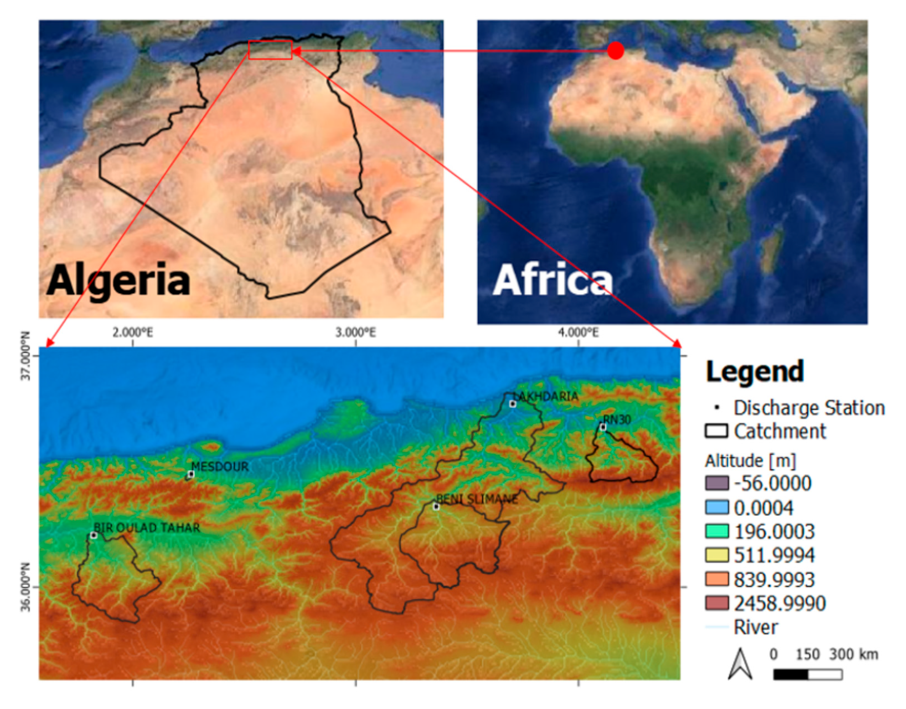
The availability, quality, and size of the climatological data play an important role in the choice of the selected watersheds. According to these criteria, five watersheds located in the northern part of Algeria were selected in our case (Figure 1), which are the Aissi, Zddine, Malah, Isser, and Boukdir catchments. These basins are characterized by a semi-arid climate with high evapotranspiration combined with low annual precipitation, as is the case for the basins of North Africa with zero flows during summer months. Table 2 shows the main properties of these basins. Two basins are influenced by the presence of dams, which is the dam of Koudiat Acerdoune upstream of the Isser basin and the Ouled Mellouk dam in the downstream part of the Zddine basin. The presence of Koudiat Acerdoune has a weak influence on the flow of water because it is considered one of the perennial rivers in Algeria with important flows, unlike Ouled Mellouk which influences a lot of river runoff, and this will be represented in the Section 3.
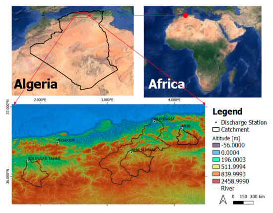
Figure 1.
Map of the study area.
Table 2.
Watershed characteristics.
2.2. Datasets
The series of climatological data used in this study over a period of 10 years (2005–2015) is summarized in daily maximum and minimum temperatures, daily streamflow, and daily precipitation, except for SM2RAIN with only the period 2007–2015 available. Table 3 represents the characteristics of 15 rain gauge stations available for the present study during the time period 2005–2015. The daily maximum and minimum temperatures are extracted from the ERA5 product due to the lack of complete meteorological station data to calculate the evapotranspiration in the different basins. Observed daily river discharge was obtained at 4 hydrometric stations from the National Agency of Hydraulic Resources (ANRH) of Algeria. Table 1 summarizes the characteristics of the hydrometric stations.
Table 3.
Characteristics of the rain gauge stations.
2.2.1. Global Precipitation Products
Different sources of global daily precipitation data are used in this work, including GPM, SM2RAIN, PERSIANN, and CHIRPS from satellite observations and the rainfall from the ERA5 reanalysis; their characteristics are in Table 4.
Table 4.
Satellite rainfall dataset characteristics.
GPM-IMERG
After the great success achieved by the Tropical Rainfall Measuring Mission (TRMM) satellite product founded by cooperation between two space agencies, the National Aeronautics and Space Administration (NASA) and the Japan Aerospace Exploration Agency (JAXA) in 1997 for 17 years, an advanced successor of TRMM was launched in February 2014 called The Global Precipitation Measurement (GPM) spacecraft; the GPM microwave imager powered by NASA and the JAXA-provided dual-frequency precipitation radar are the primary sensors of GPM, and these sensors play the role of observers of rainfall and snowfall structure and intensity [33].
These merged satellite precipitation data showed 30 min temporal resolution, 0.1° × 0.1° spatial resolution, and near-global coverage (65° N to 65° S). The extended capability to measure light rainfall (<0.5 mm), solid precipitation, and microphysical properties of precipitating particles highlights MOC over TRMM. The Integrated Multi-satellitE Retrievals for GPM (IMERG) algorithm has enabled the collection of rain and snow precipitation from space for more than 20 years from NASA’s TRMM and GPM missions by merging early precipitation estimates collected between 2000 and 2015 during TRMM satellite operations with more recent (2014–present) precipitation estimates collected during GPM satellite operations.
SM2RAIN-ASCAT
Due to the lack of consistency and scarcity of in situ observations of precipitation, a recent approach, called SM2RAIN, based on the inversion of the soil–water equilibrium equation, more precisely the water balance, uses soil moisture variations to estimate precipitation using the SM2RAIN (Soil Moisture to Rain) algorithm [34,35]. In our case, satellite-derived SM data derived from the Advanced SCATterometer (ASCAT), provided by the European Organization for the Exploitation of Meteorological Satellites (EUMETSAT) Satellite Application Service on Operational Hydrology and Water Management Support (H SAF), with a daily time step and a spatial resolution of 12.5 km, were exploited. The product covers the period 2007–2021. Several studies have adopted this satellite product in semi-arid regions and it has proven to be effective [24,28,36].
PERSIANN-CCS-CDR
The PERSIANN-CCS-CDR (Precipitation Estimation from Remotely Sensed Information using Artificial Neural Networks–Cloud Classification System–Climate Data Record) product was developed by the Center for Hydrometeorology and Remote Sensing (CHRS) at the University of California, Irvine (UCI), and provides precipitation estimates at spatial resolutions of 0.04° and temporal resolutions of 3 h from 1983 to the present over the global domain of 60° S to 60° N. As its name implies, PERSIANN applies artificial neural network (ANN) technology to determine the relationship between precipitation rates and remotely sensed cloud top temperatures measured by longwave infrared (IR) sensors on GEO satellites. PERSIANN-CCS-CDR is the latest version of the PERSIANN family of products, combining the algorithms that were used to develop PERSIANN-CCS and PERSIANN-CDR and exploiting GEO satellite information as input to provide a fine spatial–temporal precipitation dataset with a long record period. Additional details on the PERSIANN product, its origin, and characteristics can be found in [37,38].
CHIRPS
CHIRPS (Climate Hazards Group Infrared Precipitation with Station data) is a recent database that has been available since early 2014; it is a result of the collaboration of the Climate Hazards Group (CHG) of the University of California and the United States Geological Survey (USGS) [39,40]. It joins various information sources, such as satellite estimates, global rainfall climatology, and in situ observations, which is why it belongs, in part, to the family of the “satellite corrected by rain gauge” category. For more accuracy, it includes the monthly precipitation climatology CHPClim (Climate Hazards Group Precipitation Climatology), the Tropical Rainfall Measuring Mission (TRMM) product 3B42, the near-global observations from the geostationary thermal infrared satellite GEO and the MODIS satellite, the precipitation fields from the NOAA CFS (Climate Forecast System) atmospheric models, and precipitation observations from various sources [41]. CHIRPS has been available since 1981 up until today, with a spatial resolution of 0.05° and at daily time resolution scales, covering 50° S–50° N (and all longitudes).
ERA5
In the framework of the Copernicus Climate Change Service (C3S), the European Centre for Medium-Range Weather Forecasts (ECMWF) released its fifth generation of ERA-5 reanalysis in February 2019. ERA5 combines large amounts of historical observations into global estimates using advanced modeling and data assimilation systems. These systems are based on the 4D-Var data assimilation system with a modern global atmospheric model (cycle 41r2 of the Integrated Forecasting System (IFS)), which was operational at ECMWF in 2016, to integrate measurements from different observing systems (station measurements, upper air soundings, satellite radiances, etc.). This product has a spatial resolution of 31 km and an hourly temporal resolution and the period covered will be extended to 1950 in the future. ERA5 has been applied in many recent studies [2] for hydrological modeling. A more detailed review of the ERA5 configuration and how it was produced is presented in [42,43].
2.2.2. Evapotranspiration Data
In the rainfall–runoff simulation, hydrological models need other climatological parameters besides precipitation, such as temperature and potential evapotranspiration (PET). In our work, PET is calculated using the Hargreaves–Samani equation based on minimum and maximum daily temperature values extracted from the ERA5 reanalysis product. In this study, the Hargreaves–Samani equation to estimate potential evapotranspiration was chosen for its suitability to the available data and the semi-arid context of the catchments studied, particularly in regions where climatic data are limited. This method offers a simple and effective alternative and its applicability has been demonstrated in several semi-arid basins, both in Algeria and semi-arid regions [24,44,45].
2.3. Methods
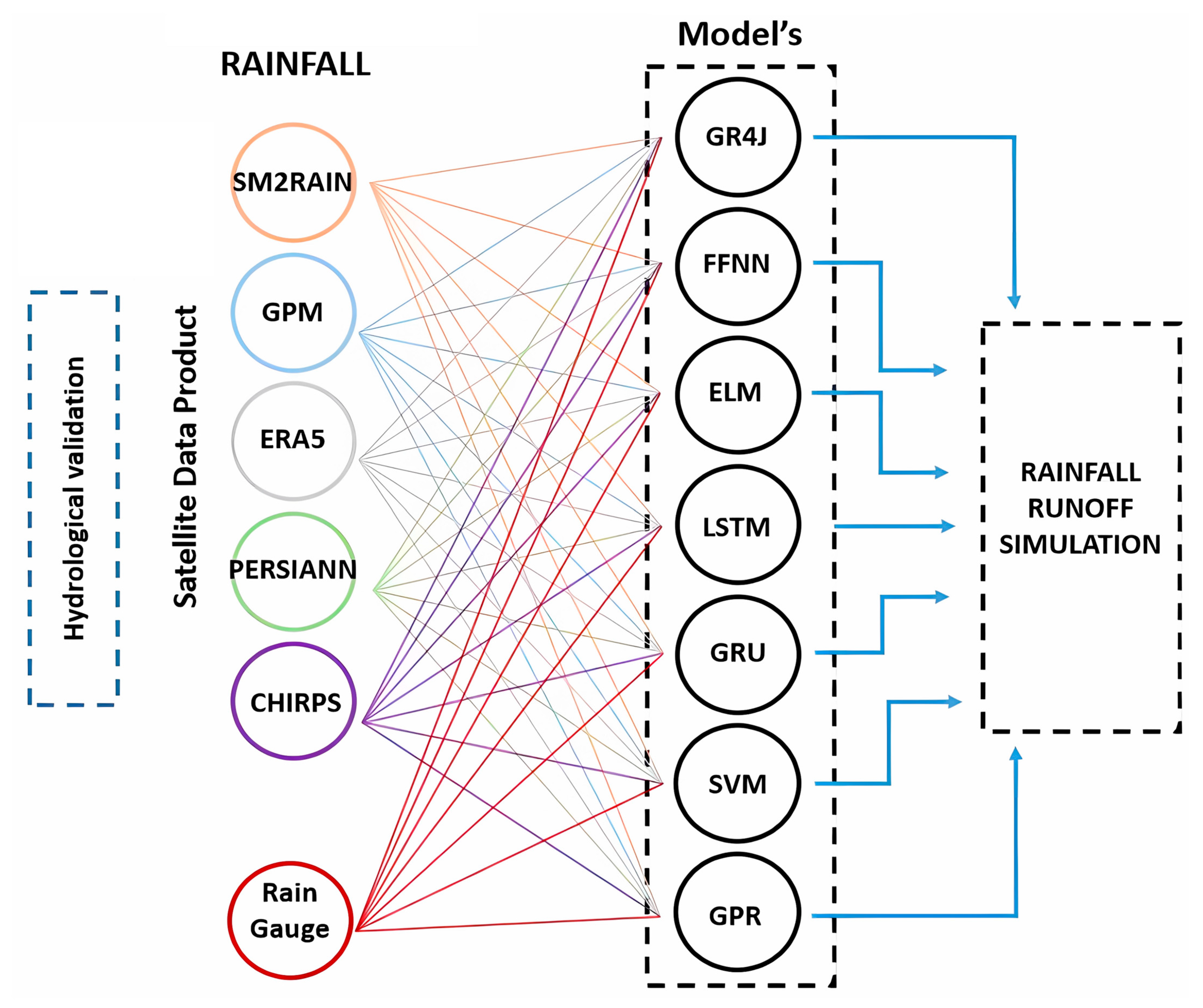
The aim of this study is to assess the ability of satellite products to predict river flow and to estimate the performance of various new modeling techniques in semi-arid regions. Hydrological validation is used to, firstly, evaluate these products by comparing the river flows estimated from satellite precipitation with the observed flows, and secondly, estimate the performance of these models by comparing the simulated flows from the models used with the observed precipitation with the flows measured at gauging stations. Figure 2 shows the different steps followed in this research. The time periods with data gaps have not been included in our analysis in order to avoid any bias linked to the processing of missing data or to a reconstruction likely to compromise the robustness of the results. We have therefore opted for the 2005–2015 period, during which the hydrometric records are complete and show minimal gaps. This period was specifically chosen to guarantee the reliability and continuity of the time series used in the modeling of rainfall and runoff, except for SM2RAIN which we used over a period from 2007 to 2015 with 85% of the data for calibration and the remaining 15% for validation.
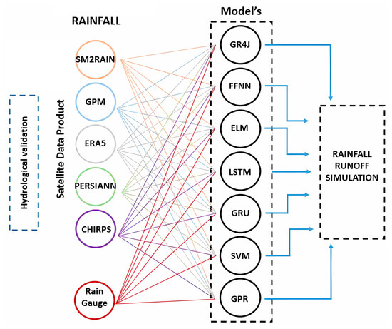
Figure 2.
The method used for rainfall–runoff simulation.
The approach adopted is based on the calibration–validation of 8 models belonging to two different families that are conceptual (GR4J and machine learning (FFNN, ELM, LSTM, LSTM2, GRU, SVM, and GPR)) with the satellite products (CHIRPS, ERA5, PERSIANN, SM2RAIN, and GPM) mentioned in the background as inputs.
2.3.1. Analysis of Catchment Response Time
When simulating the river discharge, the use of rainfall data matching the timing of river flow did not give satisfactory results in our preliminary experiments. This result is strongly linked to the way river flows are observed in these basins. These are manual stage measurements, recorded on a daily basis with a 24 h aggregation time step, which may differ from the aggregation method used for global precipitation products such as those used in the present study. In addition, the climate context of these basins in Algeria is semi-arid, with very strong modulation of river discharge during the day and the occurrence of flash floods; therefore, data at the daily time step are not the best suited to accurately report the timing of these events. This is why we have introduced a time lag between rainfall and flow to take into account these issues. Usually, the time lag is a hydrological model parameter that represents the time taken for rainwater to reach its outlet in the catchment area by passing through the hydrological system following a rainfall event, which directly affects hydrological dynamics and flow behavior. It is indeed a key parameter to improve the accuracy of hydrological forecasts. In this study, it is important to not introduce a bias in the estimation of this parameter for the reasons aforementioned, so we first used an empirical approach based on the analysis of time lags between rainfall and flows to estimate the best time lag between the time series of river discharge and rainfall.
2.3.2. Conceptual Hydrological Model (GR4J)
The “Génie Rural à 4 Paramètres Journalier” (GR4J) is one of the most widely used conceptual models in the world developed by [46] and requires 4 parameters. Two important inputs are used in this model: daily precipitation (P) and evapotranspiration (E). It is a reservoir-based model because it schematizes the watershed as a reservoir. The first reservoir is used to simulate the water balance of the soil and fills the ground reservoir. The second reservoir is used to transfer the water to the output using the routing function. This last action is divided into two parts: the 1st part is made by the 1st unit hydrograph (UH1) of an amount of 90%, and the remaining 10% of the direct runoff is made by the 2nd unit hydrograph (UH2). The simulated flow is the sum of the flows generated by UH1 and UH2.
2.3.3. Machine Learning Models
Feed-Forward Neural Network (FFNN)
The feed-forward neural network (FFNN), also called the multi-layer perceptron, is the most used architecture for artificial neural networks to manage various problems such as the forecast of a hydrological time series. The structure of this technique contains three main layers: an input layer, a hidden layer, and an output layer. To generate the desired output, first, the input data () and weights () are summed with the bias () according to Equation (1):
Second, the transfer function is applied to the result obtained by Equation (1) at the level of the hidden layer; from Equation (2), we obtain the desired output:
Before the learning procedure, the number of neurons in the hidden layer and the length of the input sequence must be fixed. During learning, the weights and biases are adjusted through the back-propagation (BP) algorithm [47]. To improve the performance of output estimates, the error between the estimated measurements and the measured values reaches predefined thresholds by an iterative task [48,49].
Extreme Learning Machine (ELM)
This recent algorithm belongs to the group of feed-forward neural networks developed by [50,51]. This method, which is extreme machine learning (ELM), is characterized by its simple structure consisting of three layers, an input, output, and a single hidden layer, unlike the feed-forward network, which uses several hidden layers. In order to generate the final output of the model, first, ELM chooses the input weights and the biases of the hidden layer in a random way; then, with the help of the least square method, we calculate the weights of the output layer instead of the iterative setting; and finally, we apply Equation (3) to obtain the final result:
We note that is the number of neurons, () is the activation function used in the model, () is the bias associated with the hidden neurons, () is the weight that connects the input layer and the hidden layer, () is the weight that connects the hidden layer and the output layer, and finally, and are the inputs and outputs, respectively, of the model.
Long Short-Term Memory (LSTM)
LSTM or long short-term memory is one of the most used neural network architectures (RNNs) in the field of deep learning [52]. This model has been improved to solve the concern of gradient vanishing or gradient exploding of the error slope in the case of a too-long time sequence encountered in RNNs, which first appeared in [53]. This structure is characterized by a memory mechanism of previous entries; its role is to help the model recognize past data to predict future data sequences. An LSTM unit consists of three gates, a forget gate, an impute gate, and an output gate, plus a memory cell (cell state) internal to the unit that serves to save, store, and maintain the outputs of the previous units for a long time. The steps of LSTM operation are, first, at the forget gate, it receives new input information and previous hidden data and it decides which information will be deleted from the cell according to Equation (4) (); then, the input gate controls which new information will be stored in the cell state. In this part, two steps are realized: the first one, which follows Equation (5) (), uses the sigmoid function () for an update to the information; the second step, summarized in Equation (6), uses the hypertangent function (tanh) to create a candidate cell () that will be used only when a new cell state is updated. The next step will combine these two cells to create a memory cell update according to Equation (7). Finally, the output gate will select the desired output using the sigmoid function according to Equation (8) which determines which part of the cell state should be output, and the product of the hypertangent function with the activated cell state () is the desired output as shown in Equation (9):
where , , and are vectors for the activation values of the forget gate, the input gate, and the output gate; , , , and are the network weights matrices; and , , , and are bias vectors.
Gated Recurrent Unit (GRU)
To speed up the training process and simplify the structure of LSTM, with the same principle as previous models, the GRU (gated recurrent unit) model has been proposed [54] in order to unite the three gates of the LSTM into only two gates. The only difference is that a GRU does not have a remotely separated memory cell or otherwise it exploits a single hidden state () by merging the hidden state and the cell state () of the LSTM cell in order to provide previous information. The operating principle of the GRU is based on two control gates: the update gate () and the reset gate (). On the one hand, the update gate serves as a tool to determine how much information will be transmitted in the future according to Equation (12); on the other hand, the reset gate helps the model to decide which data will be forgotten. In case the 2nd gate is deactivated, the GRU forgets what it has calculated previously. In order to generate the final output of the model, we go through these different calculations:
where is the input data; W and U are the network weight matrices; , , and are the hidden layer of step t, the hidden layer of step t − 1, and the present new state of step t, respectively; and and are the bias vectors.
Gaussian Process Regression (GPR)
Gaussian process regression belongs to the class of supervised machine learning algorithms that can solve nonlinear regression problems. This approach is non-parametric [55] and fully Bayesian stochastic which assumes that the probability distribution of the output is Gaussian [56]; that is, instead of computing the probability distribution of the parameterized ones of a specific function, the GPR computes the probability distribution over all admissible functions that match the data. The two essential functions to handle the Gaussian process are the mean and the covariance :
The output measure of the GPR model is calculated as follows:
where x stands for a measurement of input variables, f is the unknown functional dependence, and e is a Gaussian noise.
Support Vector Machine (SVM)
This model is also part of a set of non-parametric [57] supervised learning techniques aimed at eliminating discrimination and regression problems. SVM or wide margin separator was developed in the 1990s [58]. It uses a method called kernel function which allows for the use of linear classifiers to solve a nonlinear problem. The version of SVM that deals with regression is called Support Vector Regression (SVR). The latter is built on the principle of structural risk minimization, as it also incorporates the alternative loss function, in order to compute the existing deviations between the fitted values of the null and non-parametric models.
2.3.4. Hydrological Model Evaluation
In this study, a sequential validation approach was implemented to evaluate the performance of hydrological models in short-term streamflow prediction. This approach was divided into two main steps:
- -
- Validation with GR4J
First, the conceptual GR4J model was used. The sequential validation involves daily recalibration of the model using the available data up to the previous day (t − 1) to predict the streamflow for the following day (t). For each day in the evaluation period, the model is recalibrated based on historical data from the beginning of the training period up to i − 1. The initial conditions of the model are updated using the simulated or observed values from the previous day before generating the streamflow prediction for day i.
- -
- Validation with Machine Learning Techniques
Next, the same methodology was applied to machine learning techniques, specifically Extreme Learning Machines (ELMs) and feed-forward neural networks (FFNNs). These models use, as inputs, precipitation data at different time lags (t, t − 1, t − 2) as well as observed streamflow from previous days (t − 1 and t − 2) to predict the streamflow for day t. This strategy allows the models to account for the delayed effects of precipitation on streamflow, thereby capturing the complex hydrological dynamics of the watershed.
It is important to note that models with memory, such as long short-term memory (LSTM) and gated recurrent units (GRUs), do not use this methodology. These models inherently capture temporal dependencies and store past information, making them well suited for time series forecasting. Due to their memory-based nature, we did not apply the same sequential recalibration approach used for other machine learning models, as these models are capable of learning and adapting to the time-dependent relationships in the data without needing recalibration for each individual time step.
The performance of the GR4J, ELM, and FFNN models was assessed using standard hydrological metrics such as the Nash–Sutcliffe efficiency (NSE), the Kling–Gupta efficiency (KGE), and Root Mean Square Error (RMSE). These metrics provide a quantitative evaluation of these models’ ability to accurately reproduce observed streamflow and generate reliable predictions, which are critical for early warning systems in contexts where real-time data are limited.
2.3.5. Efficiency Criteria
After collecting the hydrometric data, which will be used for calibration and validation, the model parameters are adjusted to obtain the best possible agreement with the observed data. Once the parameters are calibrated or the model is trained, the model simulations are evaluated using independent validation data to assess its performance. Finely metrics such as Nash–Sutcliffe efficiency (NSE) and Kling–Gupta efficiency (KGE) are calculated to quantify the accuracy and performance of the model compared to observations.
Several criteria help to evaluate the predictive efficiency of the models. For our study, we used four criteria, which are Root Mean Square Error (RMSE), NSE, coefficient of determination (), and KGE, with Equations (16)–(19) shown below:
with
where Qoi and Qpi are, respectively, the observed and predicted streamflow, n is the data sample size, and are the means of observed and predicted streamflow, respectively, r is the Pearson correlation coefficient, β is the bias between observed and simulated flows, and γ is the variability ratio.
Nash–Sutcliffe efficiency (NSE) [59] is the most used criterion in the field of hydrology, when the agreement between observed and predicted values is good, its values tend to be close to 1. Root Mean Square Error (RMSE) represents the difference between measured and simulated outcomes, and the tendency of RMSE to be close to 0 means a perfect fit; if its value increases, it means that the model is less efficient. The coefficient of determination () represents the measure of the degree of reproduction of the results by the model, which is in the range of [−∞, 1]; to say that a prediction is optimal, must be close to 1. And finally, the Kling–Gupta efficiency (KGE) [60,61] is a linear combination of the three parameters of modeling errors mentioned in this section. These scores were computed only for discharge values above zero to remove the influence of intermittency and the presence of zero-flow days in the record.
2.3.6. Taylor Diagram
The Taylor diagram is a mathematical diagram whose purpose is to indicate graphically which of the different models or techniques used to model the hydrological process of the basin is the most realistic and also facilitates the comparative evaluation between the different models. Its representation is based on two shapes: the semi-circle represents positive and negative correlations and the quadrant indicates positive correlations only. The diagram is essentially based on two parameters: the correlation coefficient between the observed and simulated data and the standard deviation. A reference point (red dot) is used to indicate the accuracy of the model as a function of the position of its point; any model close to the reference point is more appropriate and more realistic.
3. Results
3.1. Impact of Time Lag Between Rainfall and Runoff on Hydrological Forecast Accuracy
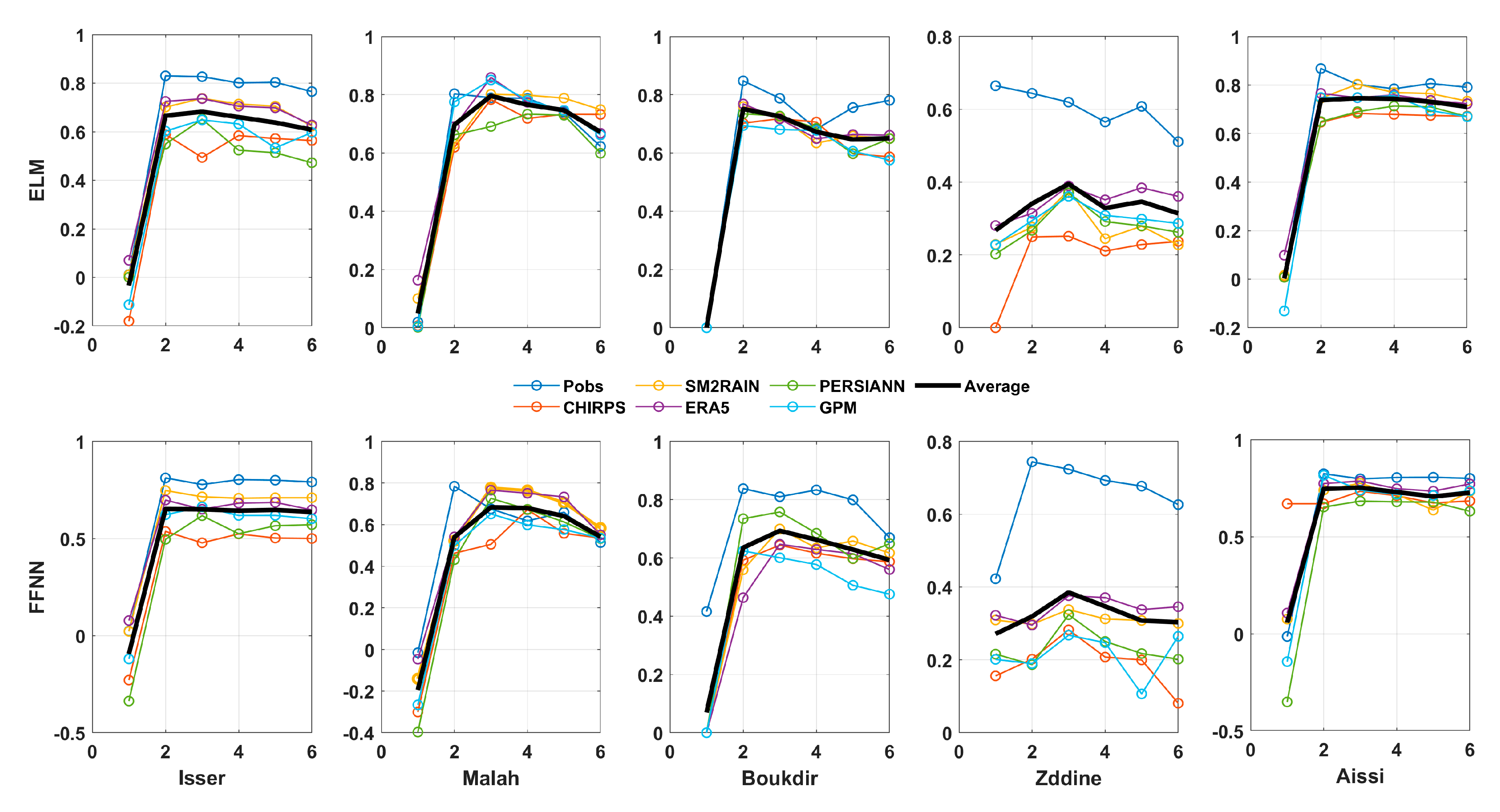
In our case, we tested several delays between one and five days (t, t − 1, t − 2, t − 3, t − 4, and t − 5) with the different rainfall inputs with the FFNN and ELM models to find out the most realistic time lag. By using the rainfall of the previous days, the model takes this delay into account and produces more accurate flow forecasts. Figure 3 shows the results obtained from the different lag times used. We have seen that the best results obtained from the observed rainfall are with the lag of the previous day (t − 1). This is most likely due to different daily data computation procedures between rainfall and river flow data. For satellite products, the best results vary between lag times t − 1 and t − 2, so we drew the black curve in Figure 3 which represents the average between the different satellite products for the different lag times. The majority of the curves show that the best results are achieved with a lag time of two days (t − 2). Consequently, we set the time lag to two days for the remainder of the study.
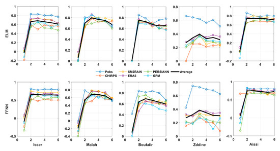
Figure 3.
Impact of time lag between rainfall and runoff on hydrological forecast accuracy.
3.2. Which Global Rainfall Product Is the Most Effective?
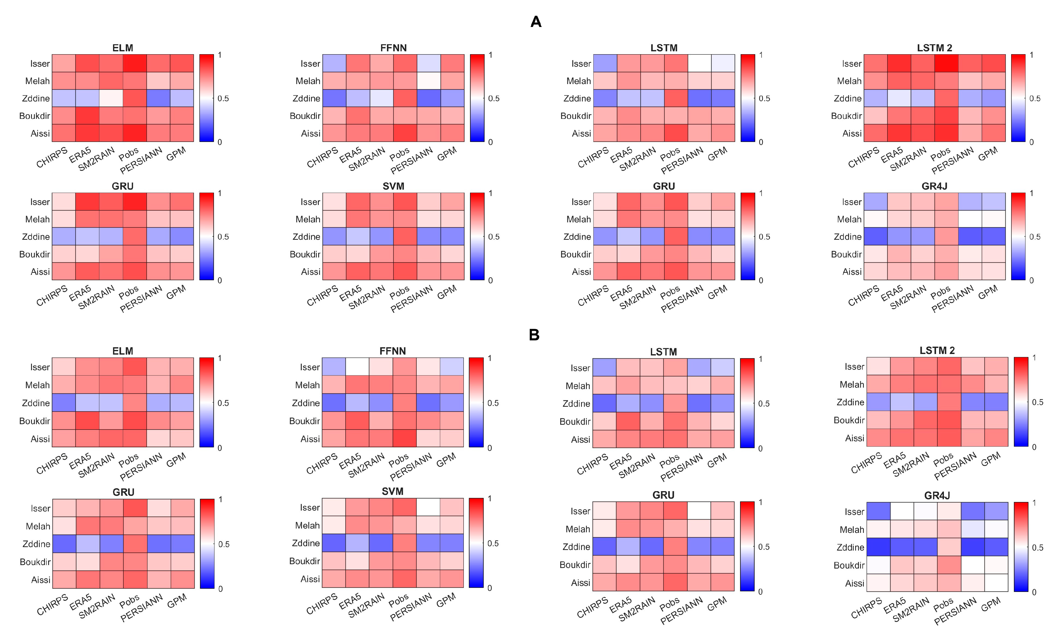
We obtained satisfactory results and significant correlations during the calibration stage, which entails adjusting the models so that they are as realistic as possible with regard to the learning information. The best KGE values recorded between Qobs and Qsim are obtained with the reanalysis product ERA5 and SM2RAIN, followed by GPM-IMERG and CHIRPS, while the least reliable product is PERSIANN, as shown in Figure 4. A good consistency of results is observed between the different basins studied, with ERA5 and SM2RAIN outperforming the others with NSE values (>0.7) only in the Zddine basin with NSE values between 0.2 and 0.4 with the FFNN, ELM, LSTM, LSTM2, GRU, SVM, GPR, CHIRPS, and GPM-IMERG ranked second with the same models with values of 0.8 ÷ 0.4 and PERSIANN ranked last with low scores in all basins. GR4J, SM2RAIN, and ERA5 demonstrated superior results to other products. In some cases, hydrological model configurations may differently represent the sequences of high or low river runoff. This highlights the need to use a variety of hydrological models when comparing different precipitation datasets in order to identify the most appropriate model to accurately illustrate local hydrographic processes. Overall, the validation process shows a slight change in scores compared with the calibration process, which is in line with expectations (Figure 4). Despite a slight decrease in correlations in some basins (such as basin 5), the performance of models such as GRU, LSTM, and FFNN remained stable between the calibration and validation stages. This indicates that these models generalized relatively well on an unseen sample of data. The validation performances of the different products used indicate that SM2RAIN and ERA5 provide the best KGE scores (0.9–0.5), with all machine learning techniques estimating runoff realistically and not underestimating it, as is the case with the other models (Figure 4). However, the initial conclusions of the evaluation suggest that the products exploiting satellite observations of soil moisture (SM2RAIN) and reanalysis products (ERA5) are proving to be very effective in detecting precipitation events in the context of near-real-time monitoring for the basins considered and that the results produced by the different inputs are not strongly influenced by the specific structures of the hydrological models used.

Figure 4.
KGE coefficient between simulated flow and observed flow of the different rainfall products for the different models. (A) is during calibration and (B) is during validation.
Observed rainfall (Pobs) is the most reliable data source, with correlations between Qobs and Qsim often greater than 0.7 for most models even with GR4J (Figure 4), both in calibration and validation. This demonstrates that the locally observed data accurately depict the dynamics of precipitation in the basins. In our case, we used Pobs as reference data, which show very small differences with the simulations obtained with SM2RAIN and ERA5. In contrast, other PPSs (CHIRPS, GPM, and PERSIANN) have failed to reproduce river discharge measurements. The effectiveness of SM2RAIN and ERA5 provides a sound alternative to rain gauge data capable of replacing observed rainfall for the catchment considered in the present study.
3.3. The Most Effective Model Structure
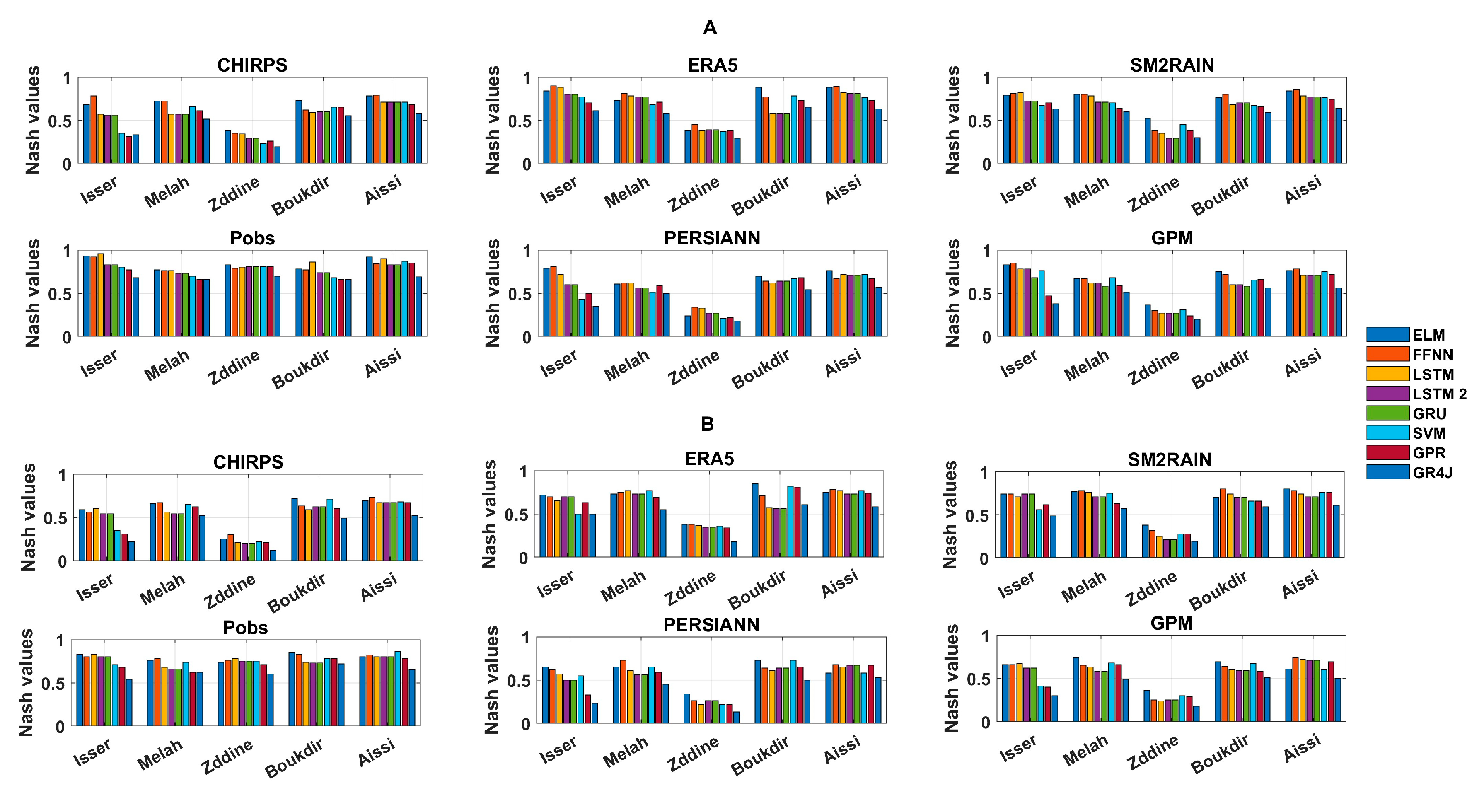
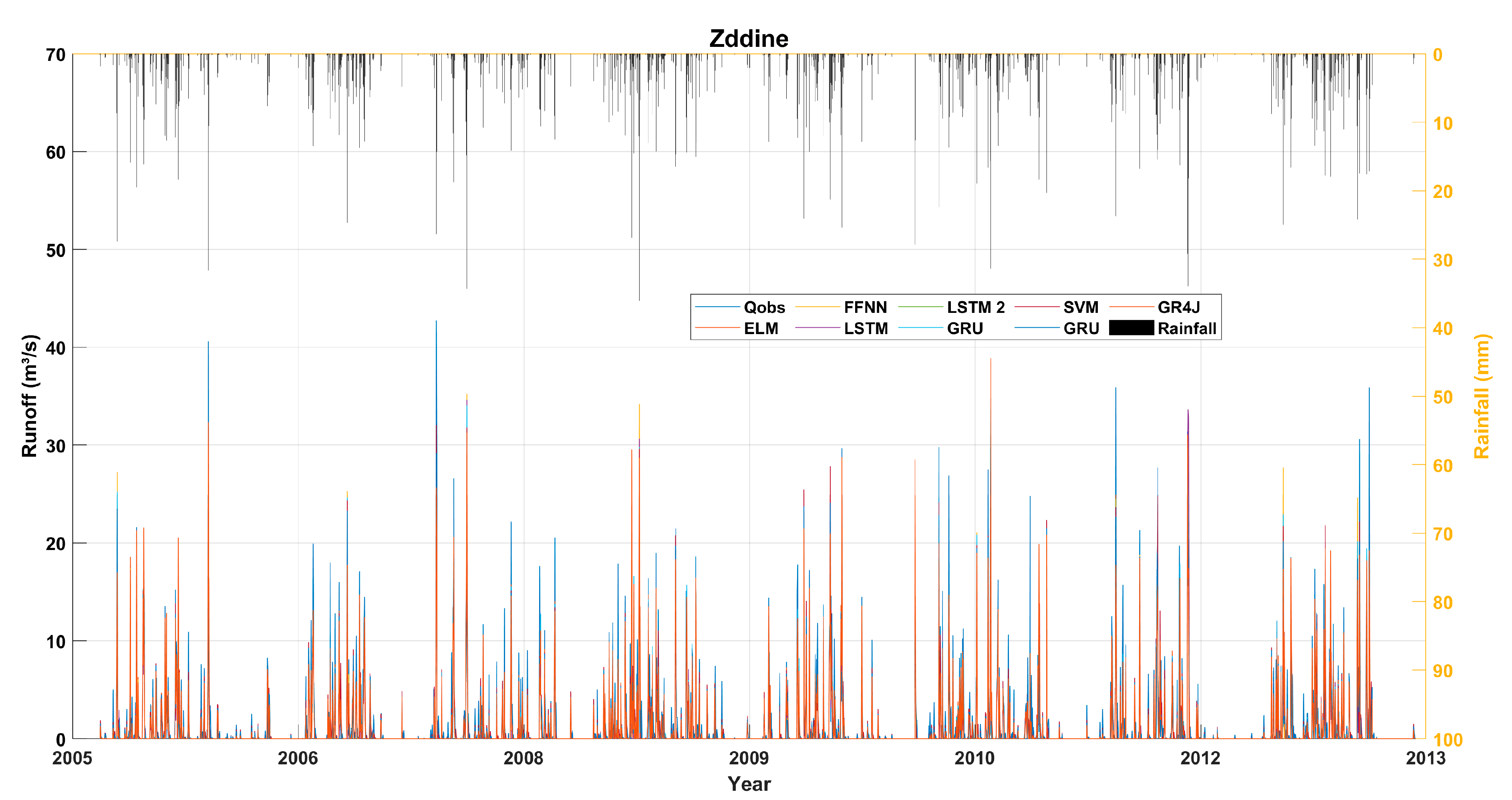
In order to determine which type of model is the most efficient and which structure is the most realistic to reproduce river runoff, Figure 5 shows the distribution of Nash values for the calibration and validation phases, respectively, obtained with the different models used for the five catchments listed in Table 1. The ELM, FFNN, LSTM, LSTM2, and GRU models generally have high correlations (>0.6), both in calibration and validation, particularly with observed rainfall and ERA5 and SM2RAIN reanalysis data. This shows that these machine learning models are able to simulate river runoff when reliable data (such as Pobs and ERA5) are used, except for the Zddine basin, where mediocre results are observed. SVM and GPR show mixed results, with moderate correlations with certain data sources, such as Pobs (around 0.7 to 0.8). However, their performance deteriorates more in validation than in some other models, particularly with precipitation data from GPM and CHIRPS. In general, the ELM, FFNN, LSTM, LSTM2, and GRU models show significant correlations (>0.6) for both calibration and validation, particularly in relation to direct precipitation observations (Pobs) and ERA5 and SM2RAIN reanalysis results. This shows that these machine learning models can efficiently reproduce observed river discharge with some rainfall inputs (such as Pobs and ERA5), except for the Zddine basin, where poor results are observed. The SVM and GPR results are mixed, showing moderate correlations with various data sources such as Pobs (around 0.5 to 0.7). Nevertheless, its validation results are poorer than those of other models, particularly with sources such as GPM and CHIRPS. The GR4J hydrological model shows poor performance compared with the machine learning models, varying between 0.1 and 0.6 in validation. This may indicate that this model is not well suited to the specific conditions of these basins, particularly for representing river intermittency, or to these types of data, especially when tested in validation.
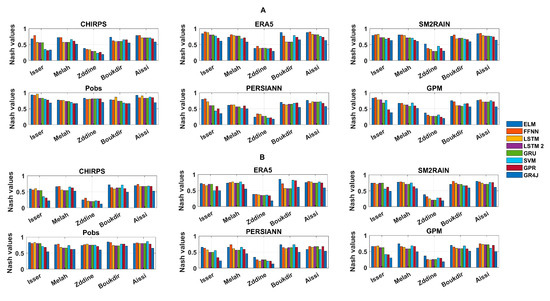
Figure 5.
Nash scores for each rainfall input in combination with the different hydrological models in calibration (A) and validation (B).
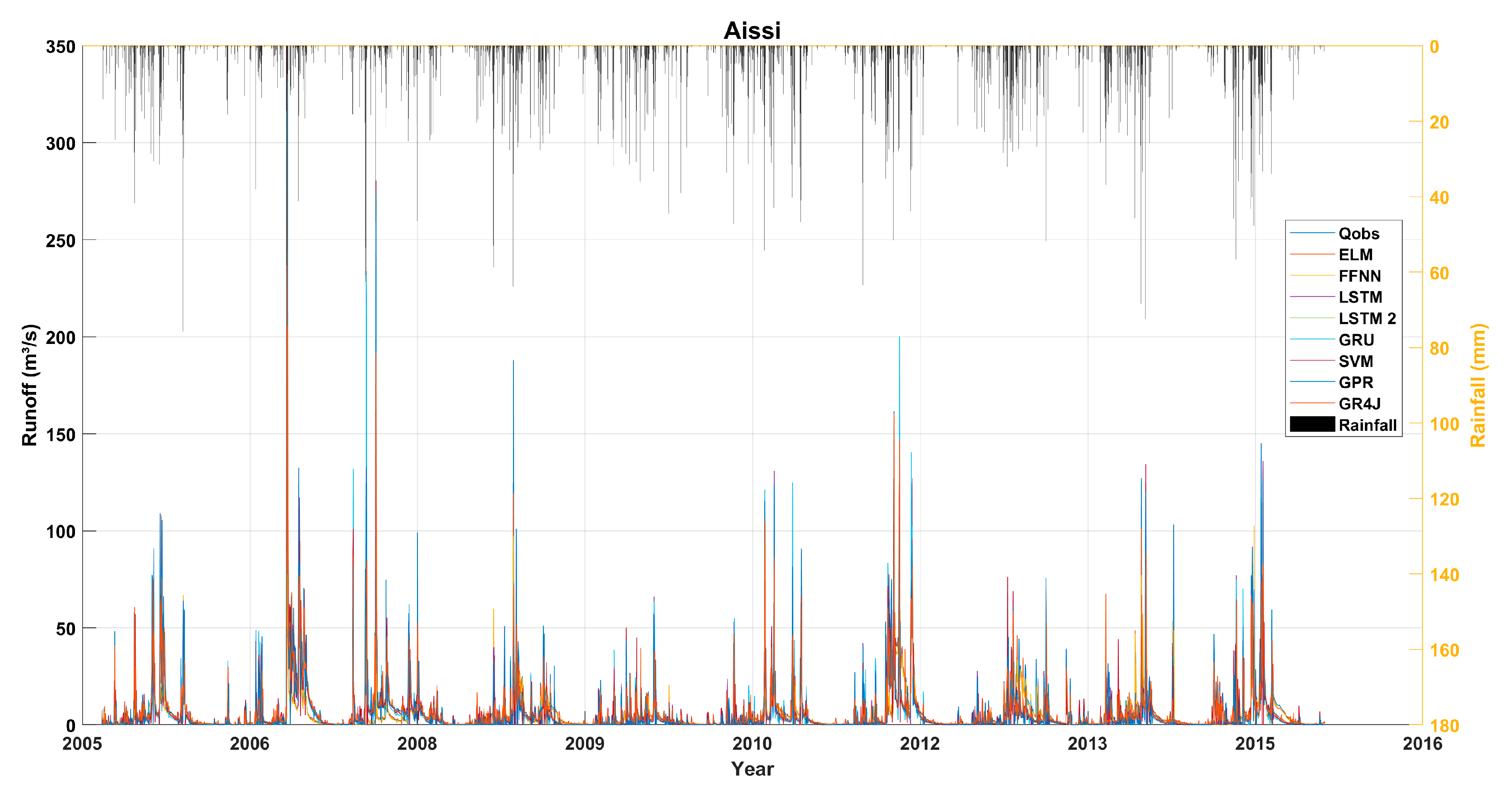
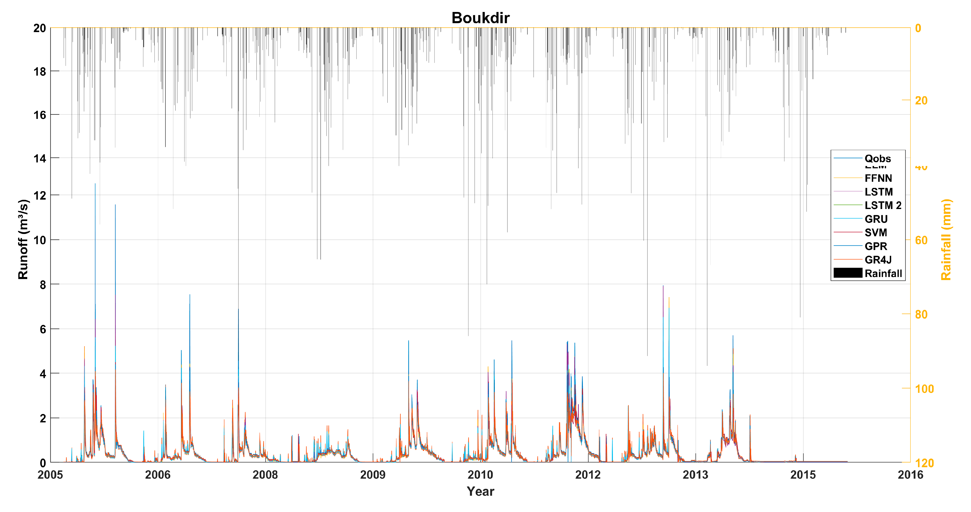
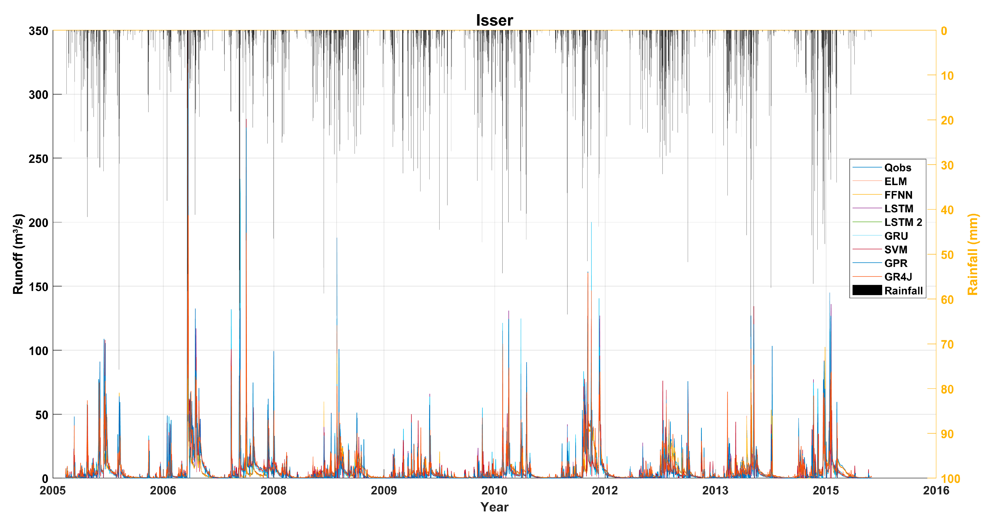
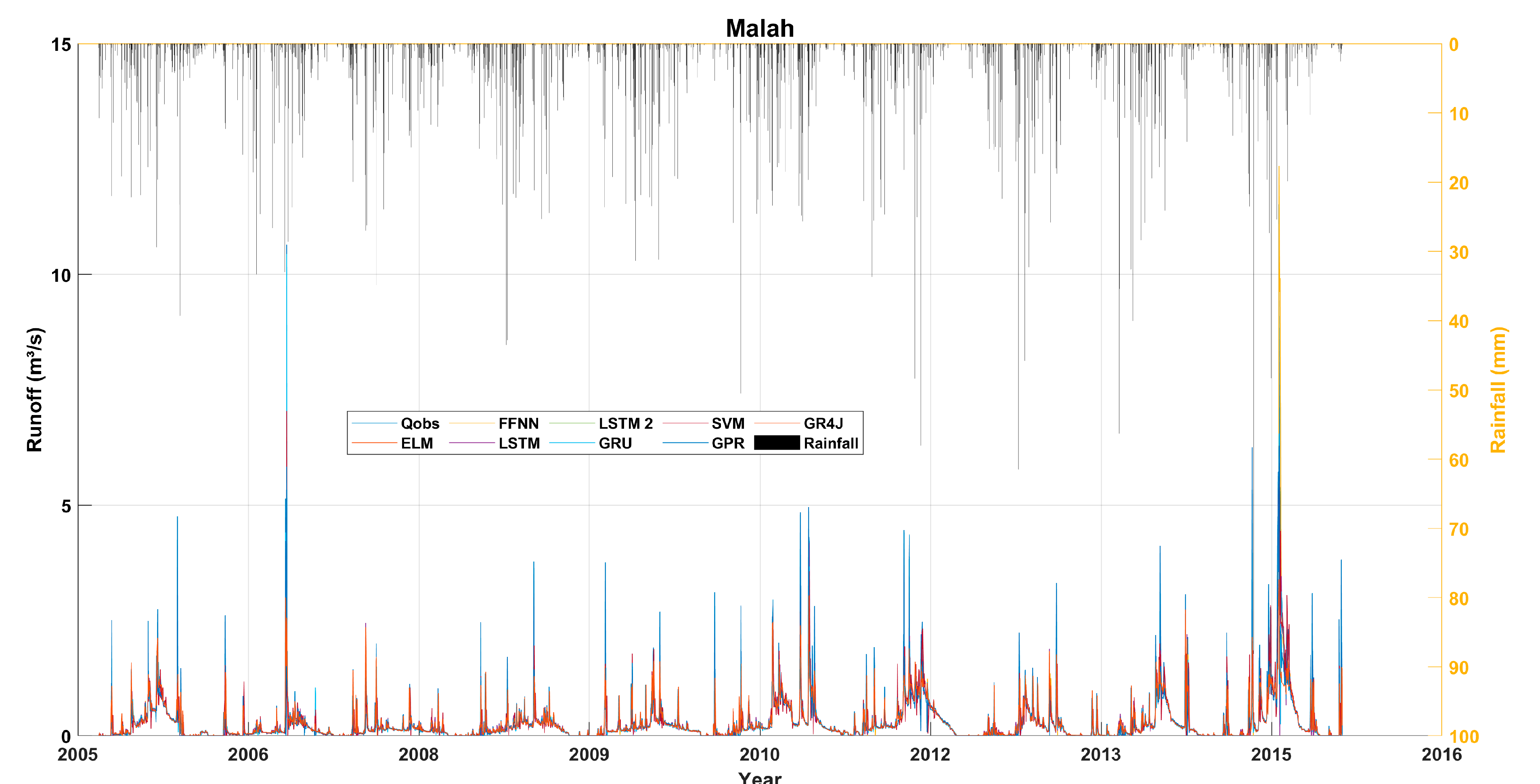
Figure 6, Figure 7, Figure 8, Figure 9 and Figure 10 shows the relationship between the flows simulated by the various models and the observed flow. There is a very good overlap with ELM, FFNN, LSTM, LSTM2, and GRU. These models capture the different peaks well, unlike GR4J, which does not manage to capture the different peaks nor the periods with very low to no runoff. Figure 7 represents all the results obtained in order to see the effectiveness of the different techniques used. This Taylor diagram (Figure 11) shows that the FFNN, ELM, LSTM, LSTM2, and GRU models perform best, as their points are closer to the reference, indicating a higher level of agreement between calculated and observed values. These observations are generalized to all the basins and all the SPs simulated with FFNN, ELM, LSTM, LSTM2, and GRU. For techniques based on basic structures (SVM and GPR), the points are between 0.4 and 0.6, unlike the results obtained with GR4j, where we notice that the points are between 0.1 and 0.4 in most instances. These observations indicate that the use of methods based on artificial intelligence makes it possible to simulate flows more realistically and accurately in the semi-arid zone. Overall, machine learning models (FFNN, ELM, LSTM, and GRU) outperform traditional hydrological models such as GR4J in their ability to capture complex precipitation dynamics and their transformation into surface runoff in these semi-arid basins.
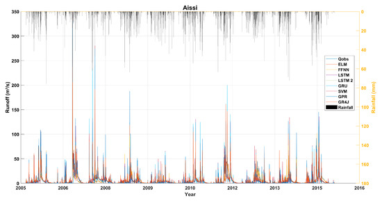
Figure 6.
Time series of observed and forecast runoff in the Aissi basin.
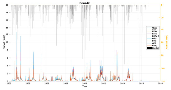
Figure 7.
Time series of observed and forecast runoff in the Boukdir basin.
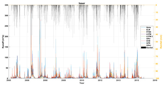
Figure 8.
Time series of observed and forecast runoff in the Aissi Isser.
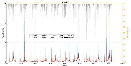
Figure 9.
Time series of observed and forecast runoff in the Malah basin.
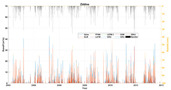
Figure 10.
Time series of observed and forecast runoff in the Zddine basin.
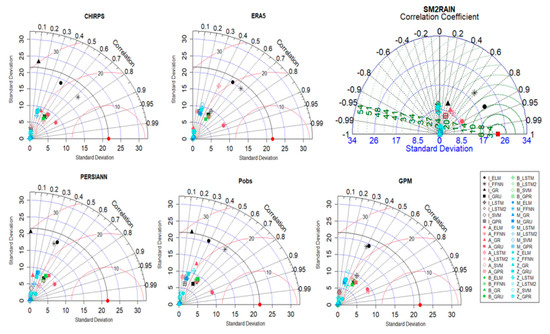
Figure 11.
Taylor diagrams for the different rainfall inputs.
4. Discussion
In this study, a hydrological evaluation was carried out for different types of precipitation data: SM2RAIN, ERA5, CHIRPS, GPM-IMERG, and PERSIANN-CCS-CDR, considering rain gauges as a reference. The objective of this comparison was to identify which product is the most suitable for the region. We also evaluated the performance of different models representing the rainfall–runoff relationship and compared the results to determine which of them (FFNN, ELM, LSTM, LSTM2, GRU, SVM, GPR, or GR4J) performed best for our region. Our study results show that SM2RAIN and ERA5 rainfall products, when combined with the ELM, FFNN, LSTM, LSTM2, and GRU models, show the best performance and consistency for calibration and validation periods.
The results presented in this study can be compared to the previous studies shown in Table 1, presented in the Section 1, which summarizes the results of recent studies evaluating the performance of satellite products in various regional and hydrological contexts. It provides an overview of the products studied, the methodological approaches adopted, and the performances obtained, with particular emphasis on their effectiveness in different regions and climatic conditions similar to Algeria. For example, products such as CHIRPS-2.0 and SM2RAIN-ASCAT stand out for their ability to accurately capture the spatio-temporal variability of precipitation in semi-arid environments, such as Pakisan and Morocco, with correlation coefficients above 0.8. In tropical zones, such as the Amazon, GPM excels in estimating intense precipitation, while SM2RAIN is highly effective for wet soils. Previous simulation tests on the evaluation of satellite products in other semi-arid regions [31,32] have also shown that PERSIANN-CCS-CDR shows the worst overall performance. Other studies in Morocco [2,24] show that SM2RAIN represents the most efficient product for this region, probably due to the low vegetation cover in this region, allowing a good satellite retrieval of soil moisture. These studies also show that the accuracy of GPM, CHIRPS, and ERA5 is higher than PERSIANN-CCS-CDR in these semi-arid regions. The integration of merged data, combining satellite observations and in situ measurements, significantly improves the performance of rainfall–runoff models, as shown by studies carried out in Turkey [30] and other regions. This picture highlights the need to choose products adapted to regional specificities and to adopt hybrid approaches to optimize rainfall estimates and hydrological modeling. The results of our research confirm that the ERA5 and SM2RAIN products offer the best performance, particularly in semi-arid regions such as the basins studied in Algeria. Their high accuracy in capturing the spatio-temporal variability in precipitation and soil moisture conditions places them at the forefront of rainfall–runoff modeling tools in these contexts. PERSIANN-CCS-CDR, on the other hand, performs less well, underlining the importance of selecting products adapted to the region and its specific hydrological characteristics.
Comparison with previous studies in various regions of the world [8,23,62] confirms the robustness of some of the AI models. These studies show that LSTM outperforms FFNN and is similar to ELM, which is the opposite in our case: LSTM performs worse than FFNN. Unfortunately, there is no other published research conducted with such models in Algeria for comparison purposes, so the present research aims to fill this knowledge gap. LSTMs undoubtedly work better in wetter areas (Asia and the USA), with a realistic simulation of base flow and seasonal dynamics notably related to snowmelt processes, whereas our basins are mostly semi-arid and intermittent (no flow during summer). Other analyses in semi-arid basins [25] have also revealed the difficulties of the GR4J model in reproducing intermittent hydrographs and the cessation of river runoff during extended periods. It should also be noted that this phenomenon of river intermittence has become more frequent in the region in recent years as a result of the temporary drying up caused by global climate change inducing higher temperatures and evapotranspiration rates, or by human activities increasing water withdrawals. This intermittency has a direct impact on the availability, quality, and quantity of observed data, as it causes gaps in the series during the drying period, which complicates model calibration and validation. It also leads to significantly increased temporal variability in flows, which makes it difficult to reproduce flow and dry periods accurately, and it can modify hydrological processes such as evaporation, infiltration, and runoff so that models lose their ability to represent these processes realistically in order to predict flows.
An important limitation of any hydrological modeling study in the Maghreb region is the human influence on the hydrological cycle. The presence of dams and irrigation systems means that the streamflow data used in the models are often strongly influenced by human activities. Indeed, we can distinguish between large dams, which are often well identified and for which we can estimate withdrawals [63], and, above all, the very large number of small-scale structures [64], notably from traditional irrigation systems [65], which can also withdraw significant quantities of water but are not well documented. For example, it has been shown that almost half of the surface flows from the Atlas Mountains can be derived from these ancestral systems [66]. Thus, representing the quantities of water withdrawn in the absence of reliable data enabling them to be measured remains a challenge [67].
5. Conclusions
This study provided the first evaluation of a machine learning algorithm together with global precipitation products for river discharge simulations over several catchments of Algeria. The aim of this study was to (1) evaluate eight models, ELM, FFNN, LSTM, LSTM2, GRU, SVM, GPR, and GR4J, in order to identify the most efficient and robust structure in North Algeria, and (2) evaluate the satellite products (SM2RAIN, GPM-IMERG, CHIRPS, and PERSIANN) and the ERA5 reanalysis product for hydrological simulation. This analysis was carried out using the hydrological validation method and compared simulated flows with observed flows. The results show that combining the ELM, FFNN, LSTM, LSTM2, and GRU models with the SM2RAIN and ERA5 products provided the most reliable and consistent calibration and validation scores, and that machine learning techniques are able to reproduce reliable and realistic river flows in Algerian basins. In addition, the use of satellite products or reanalysis data has a beneficial effect, given the small difference in the performance of certain products with rain gauges, especially with SM2RAIN-ASCAT and ERA5. Observed rainfall, SM2RAIN, and ERA5 give Nash values greater than 0.7, and it can be said that these products provide a good opportunity to complete rain gauge data due to the lack of measurements and the absence of monitoring networks in large parts of Algeria, and North Africa more generally, which directly affects model performance. Recent advances in flood risk forecasting and flow simulation have led to the development of hybrid models [68,69,70] combining conceptual models and machine learning that could be considered in further studies. These models demonstrate their effectiveness and encourage future research to make use of satellite products to improve the monitoring of river discharge for a better management of water resources.
Author Contributions
Conceptualization, R.B., H.B., T.B. and Y.T.; methodology, R.B., H.B., T.B. and Y.T.; formal analysis, R.B. and T.B.; resources, H.B. and Y.T.; data curation, R.B. and T.B.; writing—original draft preparation, R.B.; writing—review and editing, H.B., T.B. and Y.T.; supervision, H.B., T.B. and Y.T. All authors have read and agreed to the published version of the manuscript.
Funding
DGRSDT from Algeria granted support for the PhD of Rayane Bounab. Financial support for travel was granted by the IRD-IRN RHYMA.
Data Availability Statement
Data are available from the corresponding author upon reasonable request.
Conflicts of Interest
The authors declare no conflicts of interest.
References
- Gowda, C.C.; Mahesha, A.; Mayya, S.G. Development of operation policy for dry season reservoirs in tropical partially gauged river basins. Int. J. River Basin Manag. 2022, 22, 187–201. [Google Scholar] [CrossRef]
- El Khalki, E.M.; Tramblay, Y.; Massari, C.; Brocca, L.; Simonneaux, V.; Gascoin, S.; Saidi, M.E.M. Challenges in flood modeling over data-scarce regions: How to exploit globally available soil moisture products to estimate antecedent soil wetness conditions in Morocco. Nat. Hazards Earth Syst. Sci. 2020, 20, 2591–2607. [Google Scholar] [CrossRef]
- Sayama, T.; Tatebe, Y.; Tanaka, S. An emergency response-type rainfall-runoff-inundation simulation for 2011 Thailand floods. J. Flood Risk Manag. 2017, 10, 65–78. [Google Scholar] [CrossRef]
- Chen, Y.; Li, J.; Xu, H. Improving flood forecasting capability of physically based distributed hydrological models by parameter optimization. Hydrol. Earth Syst. Sci. 2016, 20, 375–392. [Google Scholar] [CrossRef]
- Unduche, F.; Tolossa, H.; Senbeta, D.; Zhu, E. Evaluation of four hydrological models for operational flood forecasting in a Canadian Prairie watershed. Hydrol. Sci. J. 2018, 63, 1133–1149. [Google Scholar] [CrossRef]
- Kan, G.; He, X.; Ding, L.; Li, J.; Liang, K.; Hong, Y. Study on applicability of conceptual hydrological models for flood forecasting in humid, semi-humid semi-arid and arid basins in China. Water 2017, 9, 719. [Google Scholar] [CrossRef]
- Hadid, B.; Duviella, E.; Lecoeuche, S. Data-driven modeling for river flood forecasting based on a piecewise linear ARX system identification. J. Process. Control 2019, 86, 44–56. [Google Scholar] [CrossRef]
- Boulmaiz, T.; Guermoui, M.; Boutaghane, H. Impact of training data size on the LSTM performances for rainfall–runoff modeling. Model. Earth Syst. Environ. 2020, 6, 2153–2164. [Google Scholar] [CrossRef]
- Roy, B.; Singh, M.P.; Kaloop, M.R.; Kumar, D.; Hu, J.-W.; Kumar, R.; Hwang, W.-S. Data-driven approach for rainfall-runoff modelling using equilibrium optimizer coupled extreme learning machine and deep neural network. Appl. Sci. 2021, 11, 6238. [Google Scholar] [CrossRef]
- Mazrooei, A.; Sankarasubramanian, A. Improving monthly streamflow forecasts through assimilation of observed streamflow for rainfall-dominated basins across the CONUS. J. Hydrol. 2019, 575, 704–715. [Google Scholar] [CrossRef]
- Ahani, A.; Shourian, M.; Rad, P.R. Performance assessment of the linear, nonlinear and nonparametric data driven models in river flow forecasting. Water Resour. Manag. 2017, 32, 383–399. [Google Scholar] [CrossRef]
- Xu, T.; Liang, F. Machine learning for hydrologic sciences: An introductory overview. WIREs Water 2021, 8, e1533. [Google Scholar] [CrossRef]
- Nearing, G.S.; Kratzert, F.; Sampson, A.K.; Pelissier, C.S.; Klotz, D.; Frame, J.M.; Prieto, C.; Gupta, H.V. What role does hydrological science play in the age of machine learning? Water Resour. Res. 2021, 57, e2020WR028091. [Google Scholar] [CrossRef]
- Alizadeh, A.; Rajabi, A.; Shabanlou, S.; Yaghoubi, B.; Yosefvand, F. Modeling long-term rainfall-runoff time series through wavelet-weighted regularization extreme learning machine. Earth Sci. Inform. 2021, 14, 1047–1063. [Google Scholar] [CrossRef]
- Tașar, B.; Üneş, F.; Varçin, H. Prediction of the rainfall—runoff relationship using neuro-fuzzy and support vector machines. In Proceedings of the Air and Water Components of the Environment 2019 Conference, Cluj-Napoca, Romania, 22–24 March 2019. [Google Scholar]
- Granata, F.; Gargano, R.; De Marinis, G. Support vector regression for rainfall-runoff modeling in urban drainage: A comparison with the epa’s storm water management model. Water 2016, 8, 69. [Google Scholar] [CrossRef]
- Xu, Y.; Hu, C.; Wu, Q.; Jian, S.; Li, Z.; Chen, Y.; Zhang, G.; Zhang, Z.; Wang, S. Research on particle swarm optimization in LSTM neural networks for rainfall-runoff simulation. J. Hydrol. 2022, 608, 127553. [Google Scholar] [CrossRef]
- Gao, S.; Huang, Y.; Zhang, S.; Han, J.; Wang, G.; Zhang, M.; Lin, Q. Short-term runoff prediction with GRU and LSTM networks without requiring time step optimization during sample generation. J. Hydrol. 2020, 589, 125188. [Google Scholar] [CrossRef]
- Abdi, I.; Meddi, M. Comparison of conceptual rainfall–runoff models in semi-arid watersheds of eastern Algeria. J. Flood Risk Manag. 2020, 14, e12672. [Google Scholar] [CrossRef]
- Zeroual, A.; Meddi, M.; Assani, A.A. Artificial Neural Network Rainfall-Discharge Model Assessment Under Rating Curve Uncertainty and Monthly Discharge Volume Predictions. Water Resour. Manag. 2016, 30, 3191–3205. [Google Scholar] [CrossRef]
- Nourani, V.; Gökçekuş, H.; Gichamo, T. Ensemble data-driven rainfall-runoff modeling using multi-source satellite and gauge rainfall data input fusion. Earth Sci. Inform. 2021, 14, 1787–1808. [Google Scholar] [CrossRef]
- Parisouj, P.; Lee, T.; Mohebzadeh, H.; Khani, H.M. Rainfall-runoff simulation using satellite rainfall in a scarce data catchment. J. Appl. Water Eng. Res. 2021, 9, 161–174. [Google Scholar] [CrossRef]
- Yeditha, P.K.; Rathinasamy, M.; Neelamsettya, S.S.; Bhattacharyab, B.; Agarwalc, A. Investigation of satellite rainfall-driven rainfall–runoff model using deep learning approaches in two different catchments in India. J. Hydroinform. 2021, 24, 16–37. [Google Scholar] [CrossRef]
- Tramblay, Y.; El Khalki, E.M.; Ciabatta, L.; Camici, S.; Hanich, L.; Saidi, M.E.M.; Ezzahouani, A.; Benaabidate, L.; Mahé, G.; Brocca, L. River runoff estimation with satellite rainfall in Morocco. Hydrol. Sci. J. 2023, 68, 474–487. [Google Scholar] [CrossRef]
- Cantoni, E.; Tramblay, Y.; Grimaldi, S.; Salamon, P.; Dakhlaoui, H.; Dezetter, A.; Thiemig, V. Hydrological performance of the ERA5 reanalysis for flood modeling in Tunisia with the LISFLOOD and GR4J models. J. Hydrol. Reg. Stud. 2022, 42, 101169. [Google Scholar] [CrossRef]
- Gadhawe, M.A.; Guntu, R.K.; Agarwal, A. Network-based exploration of basin precipitation based on satellite and observed data. Eur. Phys. J. Spéc. Top. 2021, 230, 3343–3357. [Google Scholar] [CrossRef]
- Ali, S.; Shahbaz, M. Streamflow forecasting by modeling the rainfall–streamflow relationship using artificial neural networks. Model. Earth Syst. Environ. 2020, 6, 1645–1656. [Google Scholar] [CrossRef]
- Satgé, F.; Hussain, Y.; Molina-Carpio, J.; Pillco, R.; Laugner, C.; Akhter, G.; Bonnet, M. Reliability of SM2RAIN precipitation datasets in comparison to gauge observations and hydrological modelling over arid regions. Int. J. Clim. 2020, 41, E517–E536. [Google Scholar] [CrossRef]
- Alazzy, A.A.; Lü, H.; Chen, R.; Ali, A.B.; Zhu, Y.; Su, J. Evaluation of Satellite Precipitation Products and Their Potential Influence on Hydrological Modeling over the Ganzi River Basin of the Tibetan Plateau. Adv. Meteorol. 2017, 2017, 3695285. [Google Scholar] [CrossRef]
- Akbaş, A.; Ozdemir, H. Comparing Satellite, Reanalysis, Fused and Gridded (In Situ) Precipitation Products Over Türkiye. Int. J. Climatol. 2024, 44, 5873–5889. [Google Scholar] [CrossRef]
- Anjum, M.N.; Irfan, M.; Waseem, M.; Leta, M.K.; Niazi, U.M.; Rahman, S.U.; Ghanim, A.; Mukhtar, M.A.; Nadeem, M.U. Assessment of PERSIANN-CCS, PERSIANN-CDR, SM2RAIN-ASCAT, and CHIRPS-2.0 Rainfall Products over a Semi-Arid Subtropical Climatic Region. Water 2022, 14, 147. [Google Scholar] [CrossRef]
- Najmi, A.; Igmoullan, B.; Namous, M.; El Bouazzaoui, I.; Brahim, Y.A.; El Khalki, E.M.; Saidi, M.E.M. Evaluation of PERSIANN-CCS-CDR, ERA5, and SM2RAIN-ASCAT rainfall products for rainfall and drought assessment in a semi-arid watershed, Morocco. J. Water Clim. Change 2023, 14, 1569–1584. [Google Scholar] [CrossRef]
- Skofronick-Jackson, G.; Kirschbaum, D.; Petersen, W.; Huffman, G.; Kidd, C.; Stocker, E.; Kakar, R. The Global Precipitation Measurement (GPM) mission’s scientific achievements and societal contributions: Reviewing four years of advanced rain and snow observations. Q. J. R. Meteorol. Soc. 2018, 144, 27–48. [Google Scholar] [CrossRef] [PubMed]
- Brocca, L.; Filippucci, P.; Hahn, S.; Ciabatta, L.; Massari, C.; Camici, S.; Schüller, L.; Bojkov, B.; Wagner, W. SM2RAIN–ASCAT (2007–2018): Global daily satellite rainfall data from ASCAT soil moisture observations. Earth Syst. Sci. Data 2019, 11, 1583–1601. [Google Scholar] [CrossRef]
- Brocca, L.; Massari, C.; Ciabatta, L.; Moramarco, T.; Penna, D.; Zuecco, G.; Pianezzola, L.; Borga, M.; Matgen, P.; Martínez-Fernández, J. Rainfall estimation from in situ soil moisture observations at several sites in Europe: An evaluation of the SM2RAIN algorithm. J. Hydrol. Hydromech. 2015, 63, 201–209. [Google Scholar] [CrossRef]
- Koohi, S.; Azizian, A.; Brocca, L. Spatiotemporal drought monitoring using bottom-up precipitation dataset (SM2RAIN-ASCAT) over different regions of Iran. Sci. Total. Environ. 2021, 779, 146535. [Google Scholar] [CrossRef]
- Ashouri, H.; Hsu, K.-L.; Sorooshian, S.; Braithwaite, D.K.; Knapp, K.R.; Cecil, L.D.; Nelson, B.R.; Prat, O.P. PERSIANN-CDR: Daily precipitation climate data record from multisatellite observations for hydrological and climate studies. Bull. Am. Meteorol. Soc. 2015, 96, 69–83. [Google Scholar] [CrossRef]
- Sadeghi, M.; Nguyen, P.; Naeini, M.R.; Hsu, K.; Braithwaite, D.; Sorooshian, S. PERSIANN-CCS-CDR, a 3-hourly 0.04° global precipitation climate data record for heavy precipitation studies. Sci. Data 2021, 8, 157. [Google Scholar] [CrossRef]
- Funk, C.; Peterson, P.; Landsfeld, M.; Pedreros, D.; Verdin, J.; Shukla, S.; Husak, G.; Rowland, J.; Harrison, L.; Hoell, A.; et al. The climate hazards infrared precipitation with stations—A new environmental record for monitoring extremes. Sci. Data 2015, 2, 150066. [Google Scholar] [CrossRef]
- Funk, C.C.; Peterson, P.J.; Landsfeld, M.F.; Pedreros, D.H.; Verdin, J.P.; Rowland, J.D.; Romero, B.E.; Husak, G.J.; Michaelsen, J.C.; Verdin, A.P. A quasi-global precipitation time series for drought monitoring. US Geol. Surv. Data Ser. 2014, 832, 1–12. [Google Scholar]
- Katsanos, D.; Retalis, A.; Michaelides, S. Validation of a high-resolution precipitation database (CHIRPS) over Cyprus for a 30-year period. Atmos. Res. 2016, 169, 459–464. [Google Scholar] [CrossRef]
- Hersbach, H.; Bell, B.; Berrisford, P.; Horányi, A.; Sabater, J.M.; Nicolas, J.; Radu, R.; Schepers, D.; Simmons, A.; Soci, C.; et al. Global reanalysis: Goodbye ERA-Interim, hello ERA5. ECMWF Newsl. 2019, 159, 17. [Google Scholar]
- Hersbach, H.; Bell, B.; Berrisford, P.; Hirahara, S.; Horányi, A.; Muñoz-Sabater, J.; Nicolas, J.; Peubey, C.; Radu, R.; Schepers, D.; et al. The ERA5 global reanalysis. Q. J. R. Meteorol. Soc. 2020, 146, 1999–2049. [Google Scholar] [CrossRef]
- Belkhiri, F.E. Performance evaluation of eighteen models for estimating reference evapotranspiration under subhumid conditions of Mitidja, Algeria. Rech. Agron. 2020, 19, 5–32. Available online: https://asjp.cerist.dz/en/article/148748 (accessed on 5 February 2025).
- Ndiaye, P.M.; Bodian, A.; Diop, L.; Djaman, K. Evaluation of twenty methods for estimating daily reference evapotranspiration in Burkina Faso. Physio-Géo 2017, 11, 129–146. [Google Scholar] [CrossRef]
- Perrin, C.; Michel, C.; Andréassian, V. Improvement of a Parsimonious Model for Streamflow Simulation. J. Hydrol. 2003, 279, 275–289. [Google Scholar] [CrossRef]
- Chen, L.; Sun, N.; Zhou, C.; Zhou, J.; Zhou, Y.; Zhang, J.; Zhou, Q. Flood Forecasting Based on an Improved Extreme Learning Machine Model Combined with the Backtracking Search Optimization Algorithm. Water 2018, 10, 1362. [Google Scholar] [CrossRef]
- Ghimire, S.; Deo, R.C.; Raj, N.; Mi, J. Deep solar radiation forecasting with convolutional neural network and long short-term memory network algorithms. Appl. Energy 2019, 253, 113541. [Google Scholar] [CrossRef]
- Guermoui, M.; Rabehi, A.; Benkaciali, S.; Djafer, D. Daily global solar radiation modelling using multi-layer perceptron neural networks in semi-arid region. Leonardo Electron. J. Pract. Technol. 2016, 15, 35–46. [Google Scholar]
- Huang, G.-B.; Zhou, H.; Ding, X.; Zhang, R. Extreme learning machine for regression and multiclass classification. IEEE Trans. Syst. Man Cybern. Part B Cybern. 2012, 42, 513–529. [Google Scholar] [CrossRef]
- Huang, G.-B.; Zhu, Q.-Y.; Siew, C.-K. Extreme learning machine: Theory and applications. Neurocomputing 2006, 70, 489–501. [Google Scholar] [CrossRef]
- Kratzert, F.; Klotz, D.; Brenner, C.; Schulz, K.; Herrnegger, M. Rainfall–runoff modelling using long short-term memory (LSTM) networks. Hydrol. Earth Syst. Sci. 2018, 22, 6005–6022. [Google Scholar] [CrossRef]
- Hochreiter, S.; Schmidhuber, J. Long Short-Term Memory. Neural Comput. 1997, 9, 1735–1780. [Google Scholar] [CrossRef] [PubMed]
- Chung, J.; Gulcehre, C.; Cho, K.; Bengio, Y. Empirical evaluation of gated recurrent neural networks on sequence modeling. arXiv 2014, arXiv:1412.3555. [Google Scholar]
- Grbić, R.; Kurtagić, D.; Slišković, D. Stream water temperature prediction based on Gaussian process regression. Expert Syst. Appl. 2013, 40, 7407–7414. [Google Scholar] [CrossRef]
- Rasmussen, C.E.; Williams, C.K.I. Gaussian Processes for Machine Learning, 3. Print; MIT Press: Cambridge, MA, USA, 2008. [Google Scholar]
- Hipni, A.; El-Shafie, A.; Najah, A.; Karim, O.A.; Hussain, A.; Mukhlisin, M. Daily Forecasting of Dam Water Levels: Comparing a Support Vector Machine (SVM) Model With Adaptive Neuro Fuzzy Inference System (ANFIS). Water Resour. Manag. 2013, 27, 3803–3823. [Google Scholar] [CrossRef]
- Cortes, C.; Vapnik, V. Support-vector networks. Mach. Learn. 1995, 20, 273–297. [Google Scholar] [CrossRef]
- Nash, J. River flow forecasting through conceptual models, I: A discussion of principles. J. Hydrol. 1970, 10, 398–409. [Google Scholar] [CrossRef]
- Gupta, H.V.; Kling, H.; Yilmaz, K.K.; Martinez, G.F. Decomposition of the mean squared error and NSE performance criteria: Implications for improving hydrological modelling. J. Hydrol. 2009, 377, 80–91. [Google Scholar] [CrossRef]
- Kling, H.; Fuchs, M.; Paulin, M. Runoff conditions in the upper Danube basin under an ensemble of climate change scenarios. J. Hydrol. 2012, 424–425, 264–277. [Google Scholar] [CrossRef]
- Le, X.-H.; Nguyen, D.-H.; Jung, S.; Yeon, M.; Lee, G. Comparison of Deep Learning Techniques for River Streamflow Forecasting. IEEE Access 2021, 9, 71805–71820. [Google Scholar] [CrossRef]
- Zahar, Y.; Ghorbel, A.; Albergel, J. Impacts of large dams on downstream flow conditions of rivers: Aggradation and reduction of the Medjerda channel capacity downstream of the Sidi Salem dam (Tunisia). J. Hydrol. 2008, 351, 318–330. [Google Scholar] [CrossRef]
- Sadaoui, M.; Ludwig, W.; Bourrin, F.; Le Bissonnais, Y.; Romero, E. Anthropogenic Reservoirs of Various Sizes Trap Most of the Sediment in the Mediterranean Maghreb Basin. Water 2018, 10, 927. [Google Scholar] [CrossRef]
- Remini, B.; Achour, B.; Kechad, R. Traditional techniques for increasing the discharge from qanats in Algeria. Irrig. Drain. Syst. 2011, 25, 293–306. [Google Scholar] [CrossRef]
- Ouassanouan, Y.; Fakir, Y.; Simonneaux, V.; Kharrou, M.H.; Bouimouass, H.; Najar, I.; Benrhanem, M.; Sguir, F.; Chehbouni, A. Multi-decadal analysis of water resources and agricultural change in a Mediterranean semiarid irrigated piedmont under water scarcity and human interaction. Sci. Total Environ. 2022, 834, 155328. [Google Scholar] [CrossRef]
- Tramblay, Y.; El Khalki, E.M.; Khedimallah, A.; Sadaoui, M.; Benaabidate, L.; Boulmaiz, T.; Boutaghane, H.; Dakhlaoui, H.; Hanich, L.; Ludwig, W.; et al. Regional flood frequency analysis in North Africa. J. Hydrol. 2024, 630, 130678. [Google Scholar] [CrossRef]
- Kapoor, A.; Pathiraja, S.; Marshall, L.; Chandra, R. DeepGR4J: A deep learning hybridization approach for conceptual rainfall-runoff modelling. Environ. Model. Softw. 2023, 169, 105831. [Google Scholar] [CrossRef]
- Kwon, M.; Kwon, H.-H.; Han, D. A Hybrid Approach Combining Conceptual Hydrological Models, Support Vector Machines and Remote Sensing Data for Rainfall-Runoff Modeling. Remote. Sens. 2020, 12, 1801. [Google Scholar] [CrossRef]
- Okkan, U.; Ersoy, Z.B.; Kumanlioglu, A.A.; Fistikoglu, O. Embedding machine learning techniques into a conceptual model to improve monthly runoff simulation: A nested hybrid rainfall-runoff modeling. J. Hydrol. 2021, 598, 126433. [Google Scholar] [CrossRef]

Disclaimer/Publisher’s Note: The statements, opinions and data contained in all publications are solely those of the individual author(s) and contributor(s) and not of MDPI and/or the editor(s). MDPI and/or the editor(s) disclaim responsibility for any injury to people or property resulting from any ideas, methods, instructions or products referred to in the content. |
© 2025 by the authors. Licensee MDPI, Basel, Switzerland. This article is an open access article distributed under the terms and conditions of the Creative Commons Attribution (CC BY) license (https://creativecommons.org/licenses/by/4.0/).