Abstract
This paper investigates the collection of aerosol particles (APs), ranging from 0.002 μm to 0.2 μm in diameter, by solid hydrometeors such as cloud ice, snow, and graupel. It specifically examines electrostatic scavenging (ESS) of APs and compares it with our previously studied scavenging by cloud droplets and raindrops. ESS by solid hydrometeors is contrasted with other scavenging mechanisms. The original two-moment aerosol scheme, which includes prognostic equations for the number and mass of APs within the numerical model, is employed in this work. It is concluded that ice crystals are most effective at electrostatic scavenging of APs compared to other solid hydrometeors. The reduction in the total mass of APs in the air caused by ESS from liquid hydrometeors exceeded six times the reduction caused by ESS from cloud ice after one hour of integration. ESS by solid hydrometeors increases the relative aerosol precipitation mass (RAPM) by less than 0.1%, whereas ESS by liquid hydrometeors raises RAPM by over 24%.
1. Introduction
Atmospheric aerosol particles (APs) significantly influence climate by absorbing or reflecting radiation and altering cloud properties. In addition to their impact on radiation, APs serve as condensation nuclei for cloud formation, which can consequently affect precipitation levels. Da Silva et al. [1] found that increased amounts of APs lead to a decrease in precipitation. In a climate model that includes aerosol–radiation and aerosol–cloud interactions, ref [2] observed that while the total amount of precipitation remains unchanged, there is a spatial redistribution of precipitation patterns. APs also have implications for human health, as they are linked to respiratory and cardiovascular diseases, particularly affecting children [3]. In 2019, air pollution caused 4.2 million deaths worldwide [4]. Mamadou and Pascal [5] concluded that neglecting the electrical charges of radionuclides in model calculations might result in an underestimation of soil contamination, which could lead to inadequate predictions of health risks associated with this contamination. These examples highlight why aerosols are an important area of research in contemporary science.
APs in natural environments carry electrical charges, which they can acquire either naturally or artificially. Various factors contribute to this charging process, including cosmic rays, radiation from radioactive materials present in the air or on the surface, electromagnetic radiation, atmospheric lightning, and static electricity generated by particle collisions [6]. APs collect ions produced in the atmosphere through the interaction of galactic cosmic rays with atmospheric gases. These ions form charge clusters that can grow and eventually develop into cloud droplets [7]. While galactic cosmic rays are a minor source of ions at the Earth’s surface, they become the dominant source of ions at altitudes around 20 km [8].
1.1. Motivation
To obtain sufficient knowledge about APs scavenging by cloud hydrometeors in cumulonimbus clouds, it is necessary to investigate the effect of electrostatic (ES) forces on the collection efficiency, in addition to other known mechanisms such as Brownian diffusion, thermophoresis, diffusiophoresis, turbulent diffusion, and intercept collection. It has been shown that small electric charges on droplets and APs in clouds can affect the scavenging of APs. Electrical charges on aerosol particles and droplets modify the droplet–particle collision efficiencies involved in scavenging, as well as the droplet–droplet and particle–particle collision efficiencies involved in the coalescence of droplets and particles, even in weakly electrified clouds and aerosol layers [9]. Ambaum et al. [10] studied the attractive force between drops carrying a fluctuating charge distribution. They concluded that the force increases as the charge variance increases.
Electrostatic forces are highly relevant to the removal of submicron APs because they provide an additional mechanism to capture particles that might otherwise be difficult to remove from the atmosphere. Small APs, with low inertia, easily follow air flow and are less likely to be trapped by other collection mechanisms. Electrostatic forces are especially important for APs that are larger than those readily collected by Brownian diffusion, but smaller than those for which inertial impaction is the dominant collection mechanism. These two APs size limits define the so-called Greenfield gap.
As for the APs scavenging by raindrops, numerous field observations, chamber experiments, and numerical simulations were conducted. However, not only liquid hydrometeors but also ice particles contribute to the removal of APs. Ice particles include ice or snow crystals, which grow by diffusion of water vapour on ice nuclei aerosol (deposition), or are formed from the freezing of supercooled drops through heterogeneous nucleation mechanisms. APs scavenging by snow is a more complex process than scavenging by raindrops, and depends on the shape and size of crystals or snowflakes, the ES charge, vapour, and temperature gradients between snow and the environmental air. It causes large differences in the values of collection efficiency between experimental results and theoretical models, especially for submicron APs.
Kyrö et al. [11] calculated snow scavenging coefficients for APs ranging from 10 nm to 1 μm, based on four years of measurements of the amount and intensity of precipitation and APs size spectra, without consideration of the APs charge. The median was 1.8 × 10⁻⁶ s−1, a value that was not significantly different from the scavenging coefficients for rainfall.
The knowledge that the electrostatic force significantly increases the collection efficiency for small APs (with a radius between 0.001 and 10 μm) comes from the first work by [12], which investigated the effect of ES charge on the collection efficiency of APs by ice crystals. The crystals were idealised as oblate spheroids. Murakami et al. [13] investigated the collection efficiency of charged natural snow crystals for APs of 0.1 to 6 μm in diameter. They showed that enhancement of collection efficiency due to the ES charges on snow crystals increases as the APs size decreases, with a maximum around 0.2 μm. Wang and Pruppacher [14,15] performed theoretical determinations of the efficiency of APs collection under subsaturated conditions. They found that increasing the ES charge leads to an increase in the collection efficiency.
The electroscavenging of APs by cloud water and rainwater is investigated by [16]. They explicitly calculated the efficiency with which APs less than 0.2 μm in diameter collide with cloud droplets and raindrops in the air due to the individual and combined simultaneous action of all ice nucleation and collection mechanisms, including ES forces caused by electric charges on the cloud droplets and APs. They concluded that electroscavenging by cloud droplets significantly affects the mass of APs in precipitation at the end of the integration period. At the same time, its influence on the number of APs is not so important. An important finding is that considering the charge distribution on the APs leads to a significant increase in the number and mass of APs in precipitation on the surface per square metre at the end of the integration.
For the first time, the effect of the simultaneous action of different ice nucleation mechanisms and electroscavenging on the temporal evolution of the total mass and number of APs in the air, hydrometeors, and precipitation on the surface is analysed by [17]. ES collection was only performed with liquid hydrometeors. They concluded that ES collection of APs by cloud droplets is the predominant collection mechanism for submicron APs, except for the smallest APs where Brownian diffusion dominates. The depositional nucleation scavenging mechanism, which removes APs from the air by acting as ice nuclei during depositional ice nucleation, the direct phase transition from water vapour to ice, most effectively reduces the mass of APs in the air.
1.2. Knowledge Gap
Image charge interactions between APs and both liquid and solid hydrometeors play a significant role in AP collection. Vučković et al. [16] studied AP scavenging by cloud droplets through image charge in detail. Applying the flux method results in a differential equation that cannot be solved analytically. Therefore, the kernel for electrocollection of APs by cloud droplets, when image charge is included, cannot be obtained in an analytical form suitable for use in bulk models. The solution was to divide the APs and hydrometeors into discrete bins and calculate the collection kernels separately, using the trajectory method, for all AP–hydrometeor pairs, for every possible value of the charge on the APs, and for different altitudes. These kernels could then be used in the 3D numerical cloud-resolving model as lookup tables.
It is difficult to determine how this should be conducted for crystals, which exhibit a wide variety of shapes and an electric AP charge distribution, as well as a complex image charge distribution from a point charge located near the ice surface. To the best of our knowledge, no one has applied the image charge method to cloud ice. Usually, the electrostatic collection of APs by cloud ice is investigated using parameterisations for the two most common ice crystal shapes: plates and columns. In numerical simulations of diffuse growth and accretion by hydrometeors, their shapes are usually approximated by oblate (flattened) and prolate (elongated) spheroids, respectively. There is no suitable approximation in the literature for the image charge on a spheroid due to the presence of a point charge outside the spheroid. As far as we know, there is no parameterisation of the collection coefficient of APs by ice crystals due to image charge in the literature.
1.3. Aim and Scope
As precipitation in the upper troposphere is usually solid, especially in winter, the ice crystals, snow, and graupel act as important scavengers in the atmosphere. However, this scavenging is less well known than scavenging by liquid hydrometeors, both theoretically and experimentally. Motivated by the deficiencies in the knowledge on the scavenging of APs by ice crystals, we addressed the impact of ES collection of APs by solid hydrometeors on the scavenging of APs from the air in this study. Also, all the other known collection mechanisms are taken into account. To achieve this, we calculated kernels for the ES collection of APs by solid hydrometeors, as well as the kernels for all other collection mechanisms. The Boltzmann charge distribution on APs is assumed in the calculation. An image charge is supposed to exist only for cloud droplets. We then calculated the spectral scavenging coefficients for the discrete values of submicronic APs with diameters ranging from 0.002 to 0.2 μm. These values are then compared with the values of the spectral scavenging coefficients for the other collection mechanisms to estimate the impact of ES collection by solid hydrometeors on the APs scavenging from the atmosphere. The collection kernels are calculated for discrete values of the diameters of cloud ice, snow and graupel, using the innovative approach proposed by [17]. The kernels calculated in this way are then used in a numerical model, where the scavenging coefficients, the rate of mixing ratio, and the number concentration of solid hydrometeors are also calculated. We designed several numerical experiments to analyse how ES collection of APs by solid hydrometeors affects the total mass and number of APs in the air, in all hydrometeors, and the precipitation on the surface. We intend to use the model to simulate the seeding of convective clouds with submicron-sized reagents. Therefore, we must include all possible collection mechanisms to achieve a more complete treatment of the spatial and temporal redistribution of reagents.
2. Methods
It is commonly assumed that the mean charge on hydrometeors is proportional to their surface:
where is the charge of the hydrometeor, a is the surface charge density and has a value of C m−2 for liquid hydrometeors and for graupel, while for cloud ice and snow a has a value of C m−2, and α is an empirical parameter that varies from zero, reflecting the neutral electrical conditions, to seven [18]. Charge parameter α of three and five that we used characterised the highly electrified clouds, which are the object of our research. The average magnitude of charge carried by particles of a given size in a highly electrified cloud is fairly close to the equilibrium value arising from conduction charging in the ambient electric field. Comparing the average charge of cloud droplets and raindrops that we calculated according to Equation (1) to the measured values in [19] shows very good agreement. It fully justifies the taken values of three and five for α. Value α = 7 gives the charge on the cloud droplets and raindrops that is greater than the charge values corresponding to the observed maximum values of electric field in the thunderstorm cloud [20], and because of that, we used the values of three and five as representative. According to [21], the average charge on both graupel and ice crystals is similar in magnitude to that of drops found in ordinary thunderclouds; therefore, the chosen values for α are applicable to them as well.
The diameter size range of the APs examined in this research varies between 0.002 and 0.2 μm. For these APs, Equation (1) is not suitable because it yields unrealistically small charges. The charge of these particles follows a Boltzmann charge distribution, which is shown by [22], a hypothesis that has been utilised in numerous studies [17,23,24]. While this distribution more accurately reflects natural conditions, it presents a challenge because the scavenging coefficients cannot be solved analytically. This is resolved by dividing aerosol and hydrometeor distributions into bins and calculating the collection efficiencies and spectral scavenging coefficients for discrete values of the diameters of APs and hydrometeors. APs distribution was divided into km = 200 bins with diameters from 0.002 μm to 0.2 μm. On the other hand, hydrometeor distribution was divided into nm = 100 bins. Using the expression
the electrostatic collection efficiency for the AP with diameter Dap(k) and hydrometeor x with diameter Dx(n) have to be calculated numerically. The hydrometeor–APs electrostatic collection efficiency is the result of the net action of various forces influencing the relative motion of APs and hydrometeors. Hydrometeors can be cloud water, rain, cloud ice, snow, and graupel (x = c, r, i, s, and g, respectively). is the electrostatic collection efficiency for the pair AP with diameter Dap(k) and electrostatic charge , and hydrometeor x with diameter Dx(n) and charge qx = aiαDx2; e is the elementary charge unit (e = 1.602∙10−19 C), l = (−lm, lm). The values of surface charge density for ice hydrometeors is (see Appendix A). F(k,l) represents the fraction of APs with diameter Dap(k) with l elementary charge units. In this sum for the charge, only terms originating from the oppositely charged APs and the hydrometeor are explicitly calculated.
The collection kernel , as a volume from which the hydrometeor collects APs per unit of time, for each pair of bins for the hydrometeor and APs is calculated as
where is the terminal velocity of the hydrometeor x with the diameter . Kernels for all pairs of bins of hydrometeors and APs for different altitudes, signs of the charge of the hydrometeors, and different values of α (cloud electrification level) are calculated separately and written into lookup tables.
The collection kernel is used for the calculation of the spectral scavenging coefficients (SSC) of APs by hydrometeors x due to ES collection: , where is a size distribution of the hydrometeor x. Now, the scavenging coefficients, (s−1), for the APs electrostatically collected by hydrometeors x are calculated by integrating the SSC over the APs diameter:
where is the normalised number distribution function of the APs. The scavenging ability of hydrometeors is represented by scavenging efficiency, defined as the fraction of APs collected by a hydrometeor relative to the initial number concentrations of APs in its path. The scavenging coefficient (SC) for particles of different sizes is the rate of AP washout by hydrometeors, which varies with collection efficiency, the size distributions of particles and hydrometeors, and their terminal velocities. The number distribution of APs used in the model is [25], where is the total number of APs per unit air volume, is the m-th moment of the number distribution for APs, is the parameter of the APs size distribution, and is the gamma function. The kernels are calculated for the discrete diameters of hydrometeors and APs, and because of that, the integral should be approximated by the sum.
The expressions for SC for cloud water and rainwater are given in [17] by Equations (5) and (6). The size distributions for the rainwater, cloud ice, snow, and graupel are of the same shape and correspond to the gamma distribution (Equation (A2)):
where is the total number of hydrometeor x per unit of air volume, and and are the parameters of the hydrometeor size distribution, respectively. SCs for solid hydrometeors have the same shape as for the rainwater:
The integrals have to be replaced by sums, since the kernel is not a continuous function with Dap and Dx:
This equation can be written as
where and .
After that, the cloud-resolving numerical model calculates SCs for ES collection of APs by hydrometeor.
ES collection of APs by cloud ice is researched using parameterisations for the two most common ice crystal habits observed in the atmosphere: planar and columnar ice crystals. Ice crystals have a large variety of shapes, around which the complicated flow patterns of air are established. Therefore, these two simple forms are mainly considered theoretically in the literature [12,15,26]. Kernels for the given pair of bins, the hydrometeor–APs, for these two shapes of cloud ice (ice plates, , and columns, ) are the same:
The only difference in the calculation of these two kernels is the values of the constants and , which are given in Appendix A. Kernels for snow, , and graupel, , are, respectively,
Detailed derivation of these expressions is given in Appendix A. In the numerical model, the main variables we are forecasting are the mixing ratio and the number concentration of cloud ice. These two variables are related to cloud ice as a single entity, meaning they do not exist for ice plates and ice columns separately. Because of that, we use the arithmetic mean of these two types of kernels to represent the kernel for cloud ice.
The kernels are influenced by meteorological variables such as terminal velocity, air temperature, density, and pressure, which all depend on altitude. Therefore, we calculated the kernels at 18 different heights, spaced every 500 m from the surface up to 8500 m, using air pressure, temperature, and density based on the International Standard Atmosphere. These calculated kernels are written into the lookup tables, from which the numerical model reads them. For each model point, the nearest height for which a kernel has been calculated is identified, and the corresponding variables are used to compute the scavenging coefficients. Because the vertical resolution of the model is 500 m, there are no significant deviations in height between the model point and the point at which the kernel was calculated.
The derivation of the expressions for the scavenging coefficients for the other collection mechanisms besides electrostatic collection is given in Appendix B. For cloud ice, there are Brownian diffusion, thermophoresis, and diffusiophoresis. In the case of snow, two new mechanisms are added: directional interception and inertial collection. For the graupel, the collection mechanisms are the same as for the snow, and the expressions have the same shape as for rainwater [27].
We assumed that APs in the model could act as ice nuclei. Ice forms readily on materials with a crystallographic structure similar to that of ice. One such material is silver iodide, which is widely used in cold cloud seeding operations. Therefore, the characteristics of APs in the model—activity, density, and size distribution—are set to match those of silver iodide. Primary ice nucleation from active APs can occur from vapour (by depositional and condensation-freezing nucleation) and from cloud water (by contact and immersion nucleation). Active APs can serve as contact or immersion nuclei for freezing raindrops. The fractions of injected APs that are active as deposition, condensation-freezing, and contact ice nuclei are included in the calculation of APs mixing ratios and number concentration. Further details are available in [25], Section 4.
Using all the mechanisms previously mentioned, the production terms for the APs number concentration and the APs mixing ratio in air and all hydrometeors in the numerical model are finally calculated in the following way: and , where is the time step in the model.
Figure 1 shows the SSC for cloud ice, snow, and graupel under the conditions of supersaturation and subsaturation over the ice. The range of AP diameters in this figure is broader than what we considered in this paper. The values of the mixing ratios and concentrations for cloud ice, snow, and graupel that are used in the calculations are Qi = 10−3 kg kg−1, Ni = 2.5∙108 m−3, Qs = 0.5∙10−3 kg kg−1, Ns = 15 × 104 m−3, Qg = 5∙10−3 kg kg−1, Ng = 2.5∙103 m−3. Figure 1a,b show the SSC for each collection process for cloud ice: Brownian diffusion (black), thermophoresis (red), diffusiophoresis (green), and electroscavenging for the two cases—when the main charge of the APs is proportional to the square of the effective cloud ice diameter (Es, dark blue lines) and when the main charge of the APs is distributed according to the Boltzmann distribution (Es distr, magenta lines) for two values of the parameter alpha: α = 3 and α = 5 (dashed and dash-dotted lines, respectively). The light blue line represents the total SSC due to all collection mechanisms, excluding ES collection (Net-Es). If the ES collection is included and the charge of the APs is calculated according to expression (1), the net SSC is shown as an orange line. When the Boltzmann charge distribution is applied to APs, the net SSC is the olive-coloured line. Brownian diffusion is the dominant collection process for the smallest APs from the diameter range used. For the larger APs, ES collection becomes the dominant mechanism of APs collection. The dominance is particularly pronounced when the charge of the APs is distributed according to the Boltzmann charge distribution. In this way, the ES collection of APs fills the spectral gap.
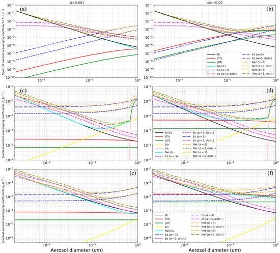
Figure 1.
Spectral scavenging coefficients for (a,b) cloud ice, (c,d) snow, and (e,f) graupel, in the conditions of supersaturation and subsaturation over the ice (left and right column, respectively). Abbrevations are as follows: Br—Brownian diffusion (black), Th—thermophoresis (red), Df—diffusiophoresis (green), Es—electroscavenging in the case when the main charge on APs is proportional to the square of the effective cloud ice diameter (dark blue lines), Es (α, distr)—electroscavenging in the case when the main charge on APs are distributed according to the Boltzmann distribution (magenta), Net-Es—the total spectral scavenging coefficient resulting from all collection mechanisms excluding electrostatic scavenging (light blue), Td—turbulent diffusion (black), Dir—directional interception (yellow), Int—inertial collection (pink). Electrostatic scavenging is calculated for two values of parameter α, α = 3 and α = 5.
In the case of snow, two new collection mechanisms are introduced: directional interception (Dir, yellow line, Figure 1c,d) and inertial collection (Int, pink line). All collection mechanisms are summarised in Table 1 and indicates which hydrometeors they apply to. The ES collection of APs is most dominant when the charge distribution is applied. ES collection is the dominant mechanism among all others when α = 5, until directional interception and inertial collection are activated. These two mechanisms become dominant for AP sizes larger than the APs considered in this study (0.002 to 0.2 μm). For α = 3, the effect of the other collection mechanism is more significant than ES collection for the smallest APs in our set of APs. Therefore, we can conclude that ES collection contributes the most to filling the Greenfield gap. For the graupel (Figure 1e,f), ES collection is again the dominant mechanism, with smaller SSC values. It can be concluded that the distribution of charge on APs makes the collection of APs more effective than in the case where the charge of APs is proportional to their surface area. The ranges of AP sizes in which ES collection dominated all other collection mechanisms for the conditions used for calculation (Qi = 10−3 kg kg−1, Ni = 2.5∙108 m−3, Qs = 0.5∙10−3 kg kg−1, Ns = 15 × 104 m−3, Qg = 5∙10−3 kg kg−1, Ng = 2.5∙103 m−3) are given in Table 2.

Table 1.
Summary of all collection mechanisms used in the investigation. The hydrometeors which they were applied to are indicated.
Table 2.
The ranges of AP diameter sizes in which ES collection dominated all other collection mechanisms for the supersaturation and subsaturation over ice.
The influence of ES collection of APs on SSCs is shown in Figure 2. The black line represents the total SSC for all collection mechanisms of APs by all hydrometeors, excluding ES collection (CTRL). When the ES collection of APs by solid hydrometeors is added to the other collection mechanisms (red lines), the SSCs are greater compared to those in CTRL. When the additional ES collection of APs by liquid hydrometeors is included (orange lines), the SSC increases significantly, especially for the larger APs in the investigated APs size range. The larger the parameter α is, the stronger this effect is. Consequently, ES collection by the solid hydrometeors affects the mass more than the number of APs. This figure shows that the ES collection of APs by solid hydrometeors contributes to filling the spectral gap. The x-axis shows the range of diameters of the APs used in the numerical model: 0.002 to 0.2 μm.
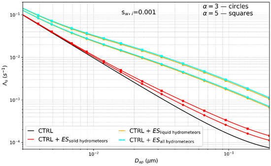
Figure 2.
The total spectral scavenging coefficients for all collection mechanisms excluding the electrostatic scavenging (ES) collection of APs (CTRL, black line); all collection mechanisms and the ES collection of APs: by solid hydrometeors (CTRL + ESsolid hydrometeors, red), by liquid hydrometeors (CTRL + ESliquid hydrometeors, orange), and all hydrometeors (CTRL + ESall hydrometeors, cyan). The calculation is performed for α = 3 (lines with circles) and α = 5 (lines with squares) in the supersaturated environment over the ice.
3. Numerical Simulations
3.1. Model Framework
For these calculations, we have used version 5.3.4 of the ARPS model (Advanced Regional Prediction System) as a basis. This model is developed by the Center for Analysis and Prediction of Storms at the University of Oklahoma [28,29] and is available for free use and further development. We have taken this opportunity to develop and implement the prognostic equations for submicron aerosols in it. This two-moment scheme for aerosols is described in detail in our previous work [25]. The three-moment microphysical scheme of [30], consisting of two liquid and four solid hydrometeor classes, is used.
3.2. Experimental Setup
The experiments are conducted under the conditions of an unstable atmosphere in which strong summer cumulonimbus develops. For this purpose, the model is initialised with the meteorological data from the radio-sounding measurements, which were characterised by a strong wind shear in the lower troposphere and a relatively high relative humidity. The cloud was initialised with an ellipsoidal bubble with a perturbed potential temperature of 4 °C. The 1.5 turbulent kinetic energy was used with the subgrid-scale turbulence parameterisation of Moeng and Wyngaard [31]. The scalar advection option is the multidimensional version of Zalesak’s flux-corrected transport scheme [32]. Open lateral boundary conditions are used. A rigid wall is assumed at the top of the domain. The domain of integration is 112 × 112 × 16 km, with a horizontal and vertical resolution of 1000 m and 500 m, respectively. The numerical simulations lasted 3 h, with a time step of 6 s.
The APs are initialised in the model in the following way. When the maximum radar reflectivity in the cloud exceeded 35 dBZ, APs were injected once into the cloud in the volume between the isotherms of 0 °C and −15 °C, where the amount of cloud and rainwater is greater than 5 × 10⁻⁴ kg kg−1. The total number and mass of injected APs was 3.84 × 10¹⁸ and 923.5 g. The mixing ratio of APs in the air was 10−11 kg kg−1 at the beginning of the seeding. The AP density used in the model is the density of silver iodide, and it is 5.67 × 10³ kg m−3. Initially, the aerosol sizes are represented by the gamma distribution previously described in [25] and shown in Figure 2 of the same article. The total AP concentrations and mixing ratios are then calculated alongside the distribution parameters in each grid point at each time step. The AP size distribution with an initial value of evolves depending on the environmental conditions and physical processes at that location. In one of the earlier papers, we showed the evolution of the mean distribution of APs over time (Figure 6 in [16]). After the first injection, no more APs are introduced into the model domain. APs either behave as passive tracers or act as ice nuclei (IN), and no AP–AP coagulation takes place. Since only a small fraction of the aerosols produced in cloud seeding practices is soluble in water, no solubility parameters were calculated, so condensation on these particles is neglected. No aerosols were present in the inertial collection region; therefore, inertial effects were neglected. The APs considered in the paper are so small that their terminal velocity can be considered negligible, so we assumed they move with the air.
We performed a series of four numerical experiments with the numerical model to explore how ES scavenging of APs by the solid hydrometeors affects the APs. The effect of electrostatic collection of APs by different hydrometeors is evaluated by analysing changes in the mass and number of APs in the air, the hydrometeors, and precipitation on the surface. To investigate how ice nucleation affects APs scavenging, these four experiments are performed twice: once when APs act as passive substances, and a second time under the same conditions, with the addition that APs serve as ice nuclei (IN), which have all the properties of silver iodide [17].
A brief overview of the experiments is provided in Table 3. EXP1 is the control experiment in which all hydrometeors (cloud droplets, raindrops, cloud ice, snow, and graupel) collect APs by various mechanisms, including Brownian diffusion, turbulent diffusion, thermophoresis, diffusiophoresis, and intercept collection, except for ES collection of APs. The effect of ES collection by the liquid hydrometeors on APs scavenging will be given in EXP2. We investigated the effect of ES collection by snow and graupel on APs scavenging and found that its influence is negligible, leading to almost identical results as in EXP1. Therefore, we concluded that only ES collection by cloud ice should be considered in EXP3. Finally, in addition to other scavenging mechanisms, ES collection of APs by all hydrometeors was considered in EXP4. In all experiments, the image charge is only present on cloud droplets. We assume that the image charge interactions between ice crystals and APs would probably not contribute significantly to the overall scavenging, since the collection of APs by cloud droplets exceeds that of other hydrometeors by at least an order of magnitude (see Figure 2). As far as we know, there is no suitable parameterisation of the collection coefficient of APs by ice crystals due to image charge in the literature. Furthermore, there is no suitable approximation for an image charge for spheroids due to a point charge, which can be used to calculate the collection coefficients of APs by the trajectory method. EXP2, EXP3, and EXP4 were performed for two values of the parameter α: α = 3 and α = 5.
Table 3.
Definitions of the numerical experiments. Yes indicates that the process is included, while No means that the process is excluded. All remaining collections (Brownian diffusion, turbulent diffusion, thermophoresis, diffusiophoresis, and intercept collection) by all hydrometeors are included in each experiment.
4. Results
The change in total mass and number of APs over time for all experiments when the APs are not acting as active ice nuclei is shown in Figure 3. This figure shows the influence of ES collection of APs by liquid and solid hydrometeors on APs from the atmosphere for α = 3 and α = 5. ES collection by liquid hydrometeors (mainly by cloud droplets) is more significant than ES collection by solid hydrometeors (mainly by cloud ice). This becomes clear in Figure 3a when looking at EXP2 and EXP3. The decrease in the total mass of APs in the air in EXP2 for α = 3 compared to the control experiment EXP1 is 8.8 times larger than in EXP3 after 1 h of integration. In EXP4, the change in APs mass in air is about 95% of the sum of the changes in APs mass in EXP2 and EXP3 at the same time. For α = 5, these values are 6.8 and 93%.
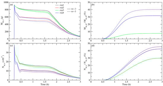
Figure 3.
Time series of the total (a) mass and (c) number of APs in the model domain in the air, and (b) the relative AP precipitation mass (RAPM) and (d) the relative AP number (RAPN) for the designated experiments for two values of the parameter α: α = 3 (solid line) and α = 5 (dashed line). APs are inactive as IN.
In EXP2, when α = 3, the total mass of APs in the air decreases by a factor that is six times greater than in EXP3 after 1.5 h of integration. In EXP4, this change in the mass of APs in the air corresponds to about 94% of the combined changes observed in EXP2 and EXP3 for the same duration. When α = 5, the changes are 4.9 times greater, which makes 90.5% of the previously mentioned combined changes.
We defined the relative aerosol precipitation mass (RAPM) as the ratio of the total precipitated AP mass (Map_pr) to the initial total mass of APs injected into the air (Map_a0). Similarly, the relative AP precipitation number (RAPN) is defined as the ratio of the total precipitated AP number (Nap_pr) to the total number of APs injected in the air (Nap_a0). These quantities were defined to analyse the impact of ES collection of APs on their scavenging. The influence of ES collection of APs by cloud ice on the RAPM is negligible for both values of the parameter α (see Figure 3b). In the EXP3 experimental setup, the RAPM at the end of the integration period is 0.03% higher for α = 3 and 0.06% higher for α = 5 than in the control experiment. Similarly, the difference between RAPM in EXP 4 and EXP 2 is also 0.04% for α = 3 and 0.1% for α = 5, indicating that ES collection of APs by solid hydrometeors has a negligible effect on RAPM. RAPM increases from 7.6% in the control experiment to 31.7% in EXP4 for α = 3 and to 40.2% for α = 5 by the end of integration. Consequently, the increase in RAPM due to ES collection of APs is solely the result of the ES collection process with cloud water.
The total number of APs present in the model domain is illustrated in Figure 3c. After 1 h of integration, the decrease in the total number of APs in the air in EXP2 is 6.6 times greater than the corresponding decrease observed in EXP3 for α = 3. For α = 5, this decrease is 4.4 times greater. After 1.5 h, these values change to 5 times and 3.6 times for α = 3 and α = 5, respectively. In EXP4, the reduction in the total number of APs in the air is approximately 93% of the sum of the reduction seen in EXP2 and EXP3 after one hour of integration for α = 3, and 87.7% for α = 5. After 1.5 h of integration, these numbers are 92% for α = 3, and 86% for α = 5. Therefore, the ES collection of APs by liquid hydrometeors is significantly more effective for scavenging APs.
The change in RAPN at the end of integration when ES collection of APs by cloud ice is included compared to the values in the control experiment for both values of α is negligible, about 0.1%. RAPN increases from 29.8% in the control experiment to 42.3% in EXP4 for α = 3 and to 45.5% for α = 5 by the end of integration. The change in RAPM at the end of integration for EXP4 is almost twice as high as the change observed in RAPN for both values of α compared to the control experiment.
In the control experiment EXP1, RAPM is significantly lower than RAPN at the end of integration. This means that in the absence of ES collection of APs, small APs are collected more compared to the larger ones. This could be assumed by looking at the SSC curve for this experiment in Figure 2 (black line). If the ES collection of APs by all hydrometeors is included, RAPM increases to 31.7% for α = 3 and to 40.2% for α = 5, i.e., to 24.1% and 32.6%, respectively. RAPN increases to 42.3% (α = 3) and 45.5% (α = 5), i.e., by 12.5% and 15.7%, respectively. From this we can conclude that in EXP4, the increase in RAPM is 1.93 (α = 3) and 2.08 times (α = 5) greater than the increase in RAPN. This is also to be expected if one considers the SSC in Figure 2 (cyan-coloured line).
Figure 4 illustrates the total mass and number of aerosols (APs) present in cloud ice and snow in the domain of integration across four experiments using two different values of the parameter α. The experimental setup in which cloud ice ES collects aerosols (EXP3) leads to an increase in both the mass and the number of APs in cloud ice and an increase in the mass of snow compared to the control experiment. This increase leads to the reduction in APs in the air and is more pronounced at a higher value of α. Remarkably, the mass of APs in cloud ice is significantly larger than in snow, almost ten times larger. Interestingly, although the mass of APs in snow is higher, their number is lower (EXP3) compared to the control experiment (EXP1). Two processes take place here. Firstly, if the cloud ice collects more APs through ES collection, a smaller number of APs remain in the air, and therefore fewer of them are collected through all other collection mechanisms except ES collection through snow. For this reason, the mass and number concentration of APs in the snow decreases. Secondly, the maximum mass of APs in cloud ice increases by more than the concentration (by a factor of 2 and 1.65 times, respectively) regarding EXP1. When part of the cloud ice is converted into snow, the mass of APs in the snow increases more than their number concentration. The result of these two processes is a greater mass of APs in the snow and a lower number concentration as a consequence of ES collection of APs by cloud ice.
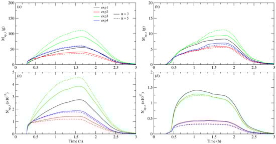
Figure 4.
Time series of the total mass and number of APs in the model domain in cloud ice (a,c) and snow (b,d) for the designated experiments for two values of the parameter α: α = 3 (solid line) and α = 5 (dashed line).
A higher value of α leads to a greater mass and fewer number of APs in the snow. Although the mass of APs is greater in cloud ice and snow, this is not reflected in the RAPM (Figure 3b). The cloud ice is at a higher altitude, so it is advected through the integration domain, and only a small amount converts into snow. In contrast, the ES collection of APs exclusively by liquid hydrometeors (EXP2) leads to a decrease in both the mass and number of APs in cloud ice and snow compared to the control experiment (EXP1), with a more pronounced decrease observed at a higher value of α.
The influence of ES collection of APs by cloud droplets on the decrease in APs number in the air, and consequently their smaller number in the cloud ice, is significantly greater than the influence of ES collection of APs by cloud ice on the increase in their number. Therefore, the number of APs in cloud ice is lower when APs are collected by all hydrometeors than in the control experiment (Figure 4c).
When ice nucleation on injected APs is considered, both the mass and the number of APs in the air decrease significantly in all experiments (see Figure 5). It appears that the ES collection of APs by cloud ice (EXP3) has no significant effect on the mass and number of APs in the air. The ES collection of APs by cloud water does not have as pronounced an effect on the ratio of aerosol particle mass (RAPM) as when the APs are passive. When APs act as reagents, both EXP2 and EXP4 show a smaller RAPM for α = 5 compared to the same experiments with passive APs. However, in the control experiment (EXP1), the RAPM value with ice nucleation is larger (15.1%) compared to the same experiments with passive APs (7.6%). The RAPN decreases in EXP2 as well as in EXP4 for both values of the parameter α. The decrease is more pronounced for α = 5 (about 9%) than for α = 3 (almost 0.1%). The influence of ES collection by all hydrometeors on RAPM and RAPN is visible in the difference between their values in EXP4 and EXP1. For the case when APs act as ice nuclei, the increase in RAPM is 16.7% (for α = 3) and 23.2% (for α = 5). The increase in RAPN is 9.7% (for α = 3) and 12.2% (for α = 5).
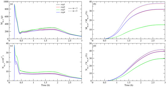
Figure 5.
Time series of the total (a) mass and (c) number of APs in the model domain in the air, and (b) the relative AP precipitation mass (RAPM) and (d) the relative AP number (RAPN) for the designated experiments for two values of the parameter α: α = 3 (solid line) and α = 5 (dashed line). APs are active as IN.
When APs are passive, the increase in RAPM is 24.2% (for α = 3) and 32.6% (for α = 5). Therefore, the larger influence on RAPM has ES collection of passive APs. The increase in RAPN is 12.6% (for α = 3) and 15.7% (for α = 5). It should be mentioned that the values of RAPN for the control experiment in these two cases at the end of integration are the same: 29.77% (passive APs) and 29.75% (APs as ice nuclei). When the APs serve as ice nuclei, the total mass is greater by 7.5% in EXP1 and by 0.1% in EXP4 for α = 3. For α = 5, however, the total mass is about 2% lower. The results shown in subfigures (b) and (d) of Figure 3 and Figure 5 are summarised in Table 4 for ease of reading. The table presents changes in RAPM (%) and RAPN (%) for the designated experiments at the end of the integration for two values of the parameter α (three and five).
Table 4.
A summary table of changes in the relative AP precipitation mass (RAPM) and the relative AP precipitation number (RAPN) for the designated experiments at the end of the integration for two values of the parameter α. In these experiments, APs are (a) inactive and (b) active as ice nuclei.
Figure 6 illustrates the total mass and number of aerosols (APs) present in cloud ice and snow in the domain of integration across four experiments, especially when ice nucleation is incorporated in all experiments. The mass of APs in snow is significantly larger when ice nucleation on APs is included than in the case of passive APs (see Figure 4). In cloud ice for EXP3, the maximum mass of APs is about six times higher than in the case without ice nucleation. However, the number of APs in the cloud ice remains almost the same as the values in Figure 4. This phenomenon is due to how AP collection is calculated. When ice nucleation is included in the model, nucleation occurs first at larger APs, followed by smaller ones, which has a greater impact on the mass than on the number of APs [25]. The maximum values of and occur very soon after the injection of APs, as you can see from the shape of the curves in Figure 6. This is a consequence of the freezing of cloud droplets due to collection of the active APs (Figure 4a in [16]). The shape of the curves representing the number of APs in cloud ice differs from those in Figure 4. It initially increases before gradually decreasing. In snow, the shape of the curve is similar to that in Figure 4, although the influence of the enhancement of AP collection by cloud ice is less significant (blue line compared to the red line). When APs act as a reagent, both the mass and concentration of APs in snow decrease when ES collection of APs is included.
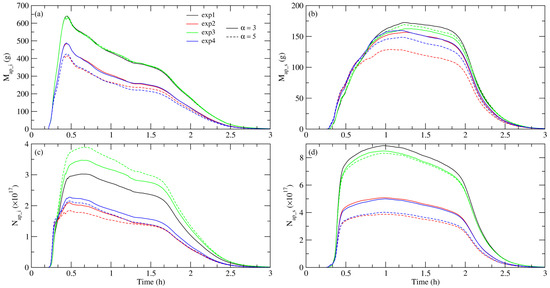
Figure 6.
Time series of the total mass and number of APs in the model domain in cloud ice ((a) and (c), respectively), and snow ((b) and (d), respectively), for the designated experiments for two values of the parameter α: α = 3 (solid line) and α = 5 (dashed line). Ice nucleation on injected APs is included.
Figure 3, Figure 4, Figure 5 and Figure 6 show the total mass and the number of APs (in the air, in various hydrometeor categories, and those precipitated on the surface) in the entire model domain.
The spatial distribution of the number of precipitated active particles (NAPs, number m−2) and their mass (MAPs, ng m−2) was assessed at the end of the control experiment (EXP1) and the experiment (EXP4) for α-values of 3 and 5 as a way to estimate the efficacy of the AP electroscavenging. These quantities are related to the surface. Two scenarios were considered in this assessment: when APs are passive (Figure 7a–c) and when they act as nuclei for cloud ice particles (Figure 7d–f).
Figure 7.
Spatial distribution of precipitated number of APs per metre squared (NAPs, ×106 m−2, isolines) and mass (MAPs, nanogram per metre squared (ng m−2), shaded) of APs at the surface at the end of integration of the control experiment EXP1, and EXP4 for α = 3 and α = 5 in the case when the APs are passive (a–c) and in the case when the APs act as nuclei for cloud ice particles (d–f).
When APs are passive, the maximum mass of APs in the control experiment is 200 ng m−2 (see Figure 7a). When ES collection of APs by all hydrometeors is included (EXP4), the maximum mass of APs is 950 ng m−2 for α = 3 and more than 1200 ng m−2 for α = 5. The conclusion is that electroscavenging increases the mass of APs in the precipitate. This is also reflected in their RAPM, which increases from 7.63% in EXP1 to 31.67% and 40.1% in EXP4 for α = 3 and α = 5, respectively (see Figure 3b). Similarly, electroscavenging increases the maximum number of APs from 1800 × 106 m−2 (EXP1) to 2800 × 106 m−2 (EXP4, α = 3) and 3000 × 106 m−2 (EXP4, α = 5). In the RAPN, the figures are as follows: 29.8% (EXP1), 42.4% (EXP4, α = 3), and 45.5% (EXP4, α = 5); see Figure 3d.
When APs are the ice nuclei, electroscavenging increases the maximum values for both the mass and the number of APs in the precipitation. The maximum mass in the control experiment is 200 ng m−2 and increases to 600 ng m−2 (EXP4, α = 3) and 950 ng m−2 (EXP4, α = 5). The RAPM is 15.1% (EXP1), 31.8% (EXP4, α = 3), and 38.4% (EXP4, α = 5). The maximum values of the number of APs in precipitation are 1800 × 106 m−2 (EXP1), 2600 × 106 m−2 (EXP4, α = 3) and 2800 × 106 m−2 (EXP4, α = 5). The RAPN in EXP1 is 29.8% (EXP1), and when including ES collection by all hydrometeors, it increases to 39.3% (EXP4, α = 3) and 42% (EXP4, α = 5).
The comparison of these two rows of Figure 7 helps us understand the effects of ice nucleation (IN) on the scavenging of APs from the atmosphere. In the control experiment, the maximum precipitated number of APs at the surface at the end of integration does not change much if the APs act as IN, and it is higher if they are passive. In EXP4, it decreases. This decrease in APs is more pronounced when α is set to 5 (3.5% decrease) than when α is set to 3 (3.1% decrease). In EXP4, the maximum mass is significantly higher when APs are passive, exceeding 1200 ng m−2 for α = 5.
5. Conclusions
The ES collection of aerosols (APs) by solid hydrometeors increases the spectral scavenging coefficients compared to situations without this collection process. The influence of ES becomes the dominant collection mechanism for larger APs. The relative increase is more pronounced for the larger AP sizes, which contributes to filling the spectral gap. However, spectral scavenging coefficients for ES collection of APs by solid hydrometeors are significantly smaller than those for the ES collection by cloud water.
Of the solid hydrometeors, cloud ice has the greatest influence on aerosol scavenging through this ES collection process, surpassing the influence of snow, hail, and graupel. However, the role of cloud ice in ES collection of APs is still less significant than that of cloud droplets. The influence of ES collection by solid hydrometeors on the relative aerosol precipitation mass (RAPM) and relative aerosol precipitation number (RAPN) is negligible due to the strong advection of cloud ice and the fact that only a small fraction of it is converted to snow.
When the injected APs serve as ice-nucleating agents, the effect of ES collection of APs on their mass and number in the air is less than in the case where they are passive tracers. The relative increase in RAPM due to ES collection of APs by all hydrometeors is greater when APs are passive tracers.
ES collection of passive APs only by cloud ice increases the mass and number of APs in cloud ice and the mass in snow, and decreases their number in snow.
ES collection by all hydrometeors increases the maximum precipitated mass and the number of APs on the surface. The maximum precipitated mass increases more than the maximum precipitated number, and these values are higher when APs are passive tracers.
The results presented in this paper highlighted the importance of including the electrostatic scavenging of APs in numerical models to improve the representation of hydrometeor–aerosol interactions.
Limitations and Future Work
The proposed approach and methodology strictly adhere to the physical formalism and the known, verified parameterisations. To our knowledge, no suitable observational data are currently available to validate the numerical results presented in this paper. We have employed the most advanced methods, utilising a comprehensive three-dimensional numerical cloud model that incorporates a detailed size-resolved three-moment microphysical scheme, a two-moment aerosol resolving scheme, and all processes recommended to enhance scavenging studies, including Brownian motion, turbulence, phoretic and electric forces, and directional interception. We have explicitly calculated the number and mass of scavenging APs at the surface and indicated their spatial distribution. However, the obtained results should be considered in light of the factors we did not take into account:
- -
- The influence of the electric field in the cloud on the supposed equilibrium charge distribution on APs. Our model does not include an electric field. However, there are very few studies addressing this in any case.
- -
- The existence of image charge on solid hydrometeors. Unlike droplets, which are spheres and for which the image charge can be calculated, for shapes differing from a sphere, such as ice crystals represented by spheroids (ellipsoids), the image charge caused by point charging outside the hydrometeor is extremely mathematically complex. As far as we know, no one has used the trajectory method to investigate the effect of image charge on electrocollection by ice crystals.
- -
- The charge distribution on hydrometeors of the same size and its spatial and temporal evolution.
- -
- Autoconversion and aggregation of APs, as well as interactions of APs with atmospheric constituents.
- -
- Change in ice nucleation characteristics of APs due to their charge.
Although field measurements of AP submicron scavenging by solid hydrometeors are scarce, some researchers [11,33] have provided their measured data of SSCs for snow scavenging. These two studies are compared in detail with combinations of different parameterizations for the distribution function, terminal velocity, and collection efficiency in [34], in order to evaluate the sensitivity of scavenging processes by snow. Zhang et al. [34] tested the scavenging sensitivity for different snowfall intensities (expressed as liquid water equivalent). SSCs in the present work correspond to the snowfall intensity of 3.9 mm h−1. Zhang et al. [34] concluded that the SSC values using [13] parameterizations, which we also used, correspond best to the aforementioned field measurements (Figure 7 in their paper). On the other hand, those parameterizations underestimated scavenging in the whole range of AP diameters compared to measurements, especially in the Greenfield gap (at least by a factor of 10). Snow SSCs (Figure 1c,d) calculated in this work show a less pronounced drop in SSC, which is a consequence of electroscavenging, and better coincide with measurements. It is important to note that our results cannot be directly compared to these measurements. Firstly, the SSC dependence on snowfall intensity is not found as stated in [11], where “we could not determine this dependency because in our dataset snowfalls were practically always similar with 95% of the intensities between 0 and 0.8 mm h−1”; therefore, their data more closely correspond to snowfall intensity of about 0.1 mm h−1. Secondly, it is known that SSC is not always positively correlated with precipitation intensity but rather represents a complex function of the mixing ratio, number concentration, and distribution functions of both hydrometeors and APs, as well as the ambient environmental conditions.
For future work, ice crystals should be approximated as spheres, and we will calculate the electrostatic collection of APs by ice crystals, including an image charge. We will use the model to test different methods of Cb cloud seeding for hail suppression.
Author Contributions
V.V.: Conceptualisation, Methodology, Software, Investigation, Writing—original draft, Visualisation, Supervision. D.V.: Conceptualisation, Investigation, Writing—original draft. D.S.: Software, Investigation, Writing—original draft. L.F.: Investigation. All authors have read and agreed to the published version of the manuscript.
Funding
This research was funded by the Science Fund of the Republic of Serbia, No. 7389, Project “Extreme weather events in Serbia—analysis, modelling and impacts”—EXTREMES.
Institutional Review Board Statement
Not applicable.
Informed Consent Statement
Not applicable.
Data Availability Statement
The original contributions presented in this study are included in the article. Further inquiries can be directed to the corresponding author.
Conflicts of Interest
The authors have no interests that are directly, or indirectly related to the work submitted for publication to disclose. The authors report there are no competing interests to declare.
List of Symbols
| Symbol | Description |
| Ice crystal columns’ axis ratio | |
| Ice crystal plates axis ratio | |
| Major semi-axis | |
| Aerosol mobility | |
| Thermophoretic factor | |
| Minor semi-axis | |
| Function for diffusiophoresis for ice crystals | |
| Cunningham’s slip factor | |
| Function for electrocollection of ice crystals | |
| Function for thermophoresis for ice crystals | |
| The specific heat of air at constant pressure | |
| Aerosol diffusivity | |
| Water vapour diffusivity in the air | |
| Diameter of hydrometeor category x | |
| Collection efficiency for AP with diameter and hydrometeor Dx(n) for l∙e charges on AP | |
| Collection efficiency for AP with diameter and hydrometeor | |
| AP collection efficiency by hydrometeor category x via mechanism y | |
| Elementary charge unit | |
| Fraction of APs with diameter with l elementary charge units | |
| Kinetic correction for thermophoresis | |
| Aerosol ventilation coefficient | |
| Ventilation coefficient for thermophoresis | |
| AP collection kernel of hydrometeor category x via mechanism y | |
| Boltzmann constant | |
| Thermal conductivity of air | |
| Thermal conductivity of AP | |
| Number of elementary charge units | |
| Molar mass of air | |
| Molar mass of water | |
| The m-th moment of the distribution of hydrometeor category x | |
| Knudsen number | |
| Reynolds number for ice crystals | |
| Concentration of aerosol particles in the air | |
| Concentration of hydrometeor category x in the air | |
| Schmidt number | |
| Normalised number concentration distribution function of APs | |
| Number concentration distribution function of hydrometeor category x | |
| Prandtl number | |
| Atmospheric pressure | |
| Charge of an aerosol particle | |
| Ice-saturated water vapour mixing ratio | |
| Charge of hydrometeor category x | |
| Ice supersaturation | |
| Liquid water supersaturation | |
| Air temperature at the hydrometeor surface | |
| Ambient air temperature | |
| Terminal velocity of hydrometeor category x | |
| An empirical parameter describing the degree of particle charging | |
| Distribution function parameters for hydrometeor category x | |
| The gamma function with parameter | |
| Terminal velocity parameters of hydrometeor category x | |
| Permittivity of free space | |
| Air kinematic viscosity | |
| Spectral AP scavenging coefficient of hydrometeor category x via mechanism y | |
| AP scavenging coefficient of hydrometeor category x via mechanism y | |
| Mean free path of air molecules | |
| Air dynamic viscosity | |
| Air density | |
| Density of hydrometeor category x |
Appendix A. Spectral Scavenging Coefficients for Electrostatic Collection
The efficiency with which some hydrometeor species x scavenge APs of specific diameter from the air can be expressed by the spectral scavenging coefficient, which is defined as the integral of a collection kernel over the hydrometeor diameters:
where denotes the collection kernel (m−3s−1) and distribution of x hydrometeor species, which can be cloud water, rainwater, cloud ice, snow, and graupel (the labels for x are c, r, i, s, and g, respectively). The scavenging coefficient is then calculated as the integral of the spectral scavenging coefficient over aerosol sizes.
The size spectrum of hydrometeor category x is described by a three-parameter gamma distribution function [35,36]:
The original expressions from the literature for collection kernels for electroscavenging of APs by cloud ice, snow, and graupel are given in Table A1.
Table A1.
The collection kernels for electroscavenging of APs by cloud ice, snow, and graupel.
Table A1.
The collection kernels for electroscavenging of APs by cloud ice, snow, and graupel.
| The Hydrometeor | Electroscavenging Kernel | Source | |
|---|---|---|---|
| Ice crystal (plates and columns) | (A3) | [12,26] | |
| Snow | (A4) | [13] | |
| Graupel | (A5) | [37] | |
- (a)
- Cloud iceIn this research, we investigated ES collection of APs by cloud ice using parameterisations for the two most common ice crystal habits: plates and columns. Their shapes were approximated by oblate and prolate spheroids, respectively. The geometrical distinction between habits can be expressed by the spheroid axis ratio (ac, bc are major and minor semi-axes), where plates have and columns .
- (a.1)
- Ice crystal platesThe initial electroscavenging kernel for ice crystal plates is presented in Table A1. Aerosol mobility is denoted with Bp and is given by the expression Cc is Cunningham’s slip factor (, , and ), with denoting AP diameter, free mean path of air molecules, and air kinematic viscosity. is APs diffusivity, is the Boltzmann constant, and is the air temperature. The ventilation coefficient is given by the equation from [20]:where is the Schmidt number, is the Reynolds number with being the ice crystal characteristic length and is the terminal velocity of the ice crystal of diameter . The terminal velocity is parameterised using the equation following [38], where is the square root of the ratio of air density at the surface and air density at the given altitude. The electrostatic interaction of AP and the ice crystal plate is represented in the term: , where and denote their electrostatic charge in Coulombs, respectively, is the permittivity of free space, . is the capacitance of the cloud ice. For the ice plates, it is calculated following [26], using the expression . For the ice columns, is , where (pp. 150–151, [39]).If we define the equivalent diameter of an ice crystal as the diameter of the sphere that has the same volume as the volume of the ice spheroid, the expression is obtained.The electric charge density of ice crystals in strongly electrified clouds can reach as high as , being ice crystal equivalent radius [15,26]. In that case, if we represent the charge of an individual crystal in the formthen should have the values . This equation will be written differently aswhere and . The value represents a non-electrified cloud, while is for highly electrified ones.We will start from the expression (A3) for the kernel given in Table A1 and substitute . The following is obtained:After that, we substituted and in the above equation, keeping in mind that is the function of and that the charge on APs is distributed by the Boltzmann distribution. The final form for the electrostatic collection kernel isIf, for the sake of brevity, we introduce the marks and ,the electrostatic collection kernel for the AP with the diameter and ice plates with a diameter finally becomes
- (a.2)
- Columnar ice crystalsFor the columnar ice crystals, the same shape of kernel as for the ice plates is obtained (Equation (A8)); only and should be replaced by and :The final result is
- (b)
- SnowThe semi-empirical expression of collection efficiency for AP scavenging by snow is given by [13], including electrocollection:Variables with subscript s correspond to those regarding snow. Electrostatic charge on snow particles is parameterised in the same manner as for ice crystals (, , and ). From this expression, we get the collection kerneland finallyTaking into account that the charge on APs is distributed following the Boltzmann charge distribution, the collection kernel for the pair of snow crystals with a diameter and APs with a diameter can be calculated using the following equation:
- (c)
- GraupelAs noted in [27], collection efficiency for graupel can be assumed to be the same as for raindrops, which are used by [37,40,41,42] (). Values for for electrocollection were taken from [37]:where . The only correction is contained in the term to take into account the porosity of the graupel, in which it is assumed that the pore space has no electric charge. The collection kernel is then calculated asHence, the collection kernel for the pair of graupel with a diameter and AP with a diameter can be calculated using the equation
Appendix B. Other Scavenging Mechanisms
Other known aerosol scavenging processes were also included in the model and are presented below.
- Ice crystals
- (a)
- Ice crystal plates
- (a.1)
- ThermophoresisThe thermophoresis collection kernel is given in the work of [12] and follows from (A1)where . Hence, the spectral scavenging coefficient can be derived:where , , . This finally gives us the following scavenging coefficient:Integral is resolved using Gauss–Laguerre quadrature.
- (a.2)
- DiffusiophoresisIn the same paper, the diffusiophoresis collection kernel iswhere , which is used to derive the spectral scavenging coefficient as follows:where and . The scavenging coefficient is thenIntegral is resolved using Gauss–Laguerre quadrature.
- (a.3)
- Brownian diffusionBy assuming spherical geometry of ice crystals, we can derive the collection kernels with expression [20]:which gives us the scavenging coefficients
- (b)
- Columnar ice crystals
- (b.1)
- ThermophoresisSimilarly, using parameterisation, explained in detail in the paper by [15], we can derive the thermophoretic scavenging coefficient for columnsIn Equation (A34), the term is equal to from (A25).Integral is resolved using Gauss–Laguerre quadrature.
- (b.2)
- DiffusiophoresisThe diffusiophoretic scavenging coefficient is then in the formIn Equation (A37), the term is equal to from (A28).Integral is resolved using Gauss–Laguerre quadrature.
- (b.3)
- Brownian diffusionEquations regarding AP scavenging by columnar ice crystals are identical to those explained in (a.3) in Appendix B, Equations (A30)–(A32).
- SnowThe semi-empirical expression for the collection efficiency of snow crystals is presented by [13]. In addition, [20] gave expressions for collection efficiency for phoretic forces.
- (c.1)
- Brownian/turbulent diffusionBrownian/turbulent diffusion collection efficiency and collection kernels are given in the following form [13]:To simplify, we used [43] which is used to derive the following scavenging coefficient:
- (c.2)
- Directional interceptionDirectional interception is parameterised as follows [13]:
- (c.3)
- Inertial impactionSimilarly, inertial impaction is derived [44]:where is the Stokes number, and the approximate formula for it comes from [43].Integral is resolved using Gauss–Laguerre quadrature.
- (c.4)
- ThermophoresisThe methodology for parameterising the thermophoretic collection kernel for ice crystal columns is adopted from [20]:where is the Prandtl number and .Integral is resolved using Gauss–Laguerre quadrature.
- (c.5)
- DiffusiophoresisDiffusiophoresis is parameterised in the following way [20]:
- GraupelAs mentioned previously in Appendix B, ref [27] advised using the raindrops collection efficiency for graupel (). Following this methodology, the scavenging coefficients for graupel are derived in the same way as for raindrops, which is explained in detail in [25].
References
- Silva, N.D.; Mailler, S.; Drobinski, P. Aerosol indirect effects on summer precipitation in a regional climate model for the Euro-Mediterranean region. Ann. Geophys. 2018, 36, 321–335. [Google Scholar] [CrossRef]
- López-Romero, J.M.; Montávez, J.P.; Jerez, S.; Lorente-Plazas, R.; Palacios-Peña, L.; Jiménez-Guerrero, P. Precipitation response to aerosol–radiation and aerosol–cloud interactions in regional climate simulations over Europe. Atmos. Chem. Phys. 2021, 21, 415–430. [Google Scholar] [CrossRef]
- UNICEF. Clear the Air for Children (The Impact of Air Pollution on Children). 2016. Available online: https://www.unicef.org/reports/clean-air-children (accessed on 20 September 2025).
- Sagheer, U.; Al-Kindi, S.; Abohashem, S.; Phillips, C.T.; Rana, J.S.; Bhatnagar, A.; Gulati, M.; Rajagopalan, S.; Kalra, D.K. Environmental pollution and cardiovascular disease. JACC Adv. 2024, 3, 100805. [Google Scholar] [CrossRef] [PubMed]
- Mamadou, S.; Pascal, L. Influence of electric charges on the washout efficiency of atmospheric aerosols by raindrops. Ann. Nucl. Energy 2016, 93, 107–113. [Google Scholar] [CrossRef]
- Zhang, L.; Gu, Z.; Yu, C.; Zhang, Y.; Cheng, Y. Surface charges on aerosol particles—Accelerating particle growth rate and atmospheric pollution. Indoor Built Environ. 2016, 25, 437–440. [Google Scholar] [CrossRef]
- Rawal, A.; Tripathi, S.N.; Michael, M.; Srivastava, A.K.; Harrison, R.G. Quantifying the importance of galactic cosmic rays in cloud microphysical processes. J. Atmos. Solar-Terr. Phys. 2013, 102, 243–251. [Google Scholar] [CrossRef]
- Nicoll, K.A.; Harrison, R.G. Stratiform cloud electrification: Comparison of theory with multiple incloud measurements. Q. J. R. Meteorol. Soc. 2016, 142, 2679–2691. [Google Scholar] [CrossRef]
- Tinsley, B.A.; Zhou, L.; Plemmons, A. Changes in scavenging of particles by droplets due to weak electrification in clouds. Atmos. Res. 2006, 79, 266–295. [Google Scholar] [CrossRef]
- Ambaum, M.H.P.; Auerswald, T.; Eaves, R.; Harrison, R.G. Enhanced attraction between drops carrying fluctuating charge distributions. Proc. R. Soc. A Math. Phys. Eng. Sci. 2022, 478, 20210714. [Google Scholar] [CrossRef]
- Kyrö, E.M.; Grönholm, T.; Vuollekoski, H.; Virkkula, A.; Kulmala, M.; Laakso, L. Snow scavenging of ultrafine particles: Field measurements and parameterization. Boreal Environ. Res. 2009, 14, 527–538. [Google Scholar] [CrossRef]
- Martin, S.J.; Wang, P.K.; Pruppacher, H.R. A Theoretical Determination of the Efficiency with which Aerosol Particles are Collected by Simple Ice Crystal Plates. J. Atmos. Sci. 1980, 37, 1628–1638. [Google Scholar] [CrossRef]
- Murakami, M.; Magono, C.; Kikuchi, K. Experiments on Aerosol Scavenging by Natural Snow Crystals Part III. The Effect of Snow Crystal Charge on Collection Efficiency. J. Meteorol. Soc. Jpn. 1985, 63, 1127–1138. [Google Scholar] [CrossRef][Green Version]
- Wang, P.K.; Pruppacher, H.R. On the efficiency with which aerosol particles of radius less than 1 μm are collected by columnar ice crystals. Pure Appl. Geophys. 1980, 118, 1090–1108. [Google Scholar] [CrossRef]
- Miller, N.L.; Wang, P.K. Theoretical determination of the efficiency of aerosol particle collection by falling columnar ice crystal. J. Atmos. Sci 1989, 46, 1656–1663. [Google Scholar] [CrossRef]
- Vučković, V.; Vujović, D.; Savić, D. Influence of electrostatic collection on scavenging of submicron-sized aerosols by cloud droplets and raindrops. Aerosol Sci. Technol. 2023, 57, 1154–1173. [Google Scholar] [CrossRef]
- Vučković, V.; Vujović, D.; Savić, D.; Filipović, L. Impact of electro-collection and ice nucleation on aerosol scavenging. Aerosol Sci. Technol. 2025, 59, 1006–1026. [Google Scholar] [CrossRef]
- Wang, X.; Zhang, L.; Moran, M.D. Uncertainty assessment of current size-resolved parameterizations for below-cloud particle scavenging by rain. Atmos. Chem. Phys. 2010, 10, 5685–5705. [Google Scholar] [CrossRef]
- Takahashi, T. Measurement of electric charge of cloud droplets, drizzle and raindrops. Rev. Geophys. 1973, 11, 903–924. [Google Scholar] [CrossRef]
- Pruppacher, H.R.; Klett, J.D. Microphysics of Clouds and Precipitation, 2nd ed.; Oxford University Press: Oxford, UK, 2010; p. 954. [Google Scholar]
- Takahashi, T.; Tajiri, T.; Sonoi, Y. Charges on graupel and Snow Crystals and the Electrical Structure of Winter Thunderstorms. J. Atmos. Sci. 1999, 56, 1561–1578. [Google Scholar] [CrossRef]
- Ghosh, K.; Tripathi, S.N.; Joshi, M.; Mayya, Y.S.; Khan, A.; Sapra, B.K. Model studies on coagulation of charged particles and comparison with experiments. J. Aerosol Sci. 2017, 105, 35–47. [Google Scholar] [CrossRef]
- Fuchs, N.A. On the stationary charge distribution on aerosol particles in a bipolar ionic atmosphere. Geofis. Pura Appl. 1963, 56, 185–193. [Google Scholar] [CrossRef]
- Ghosh, K.; Tripathi, S.N.; Joshi, M.; Mayya, Y.S.; Khan, A.; Sapra, B.K. Effect of charge on aerosol microphysics of particles emitted from a hot wire generator: Theory and experiments. Aerosol Sci. Technol. 2021, 55, 1084–1098. [Google Scholar] [CrossRef]
- Vučković, V.; Vujović, D.; Jovanović, A. Aerosol parameterisation in a three-moment microphysical scheme: Numerical simulation of submicron-sized aerosol scavenging. Atmos. Res. 2022, 273, 106148. [Google Scholar] [CrossRef]
- Martin, J.; Wang, P.K.; Pruppacher, H.R. A Theoretical Study of the Effect of Electric Charges on the Efficiency with Which Aerosol Particles are Collected by Ice Crystal Plates. J. Colloid Interface Sci. 1980, 78, 44–56. [Google Scholar] [CrossRef]
- Alheit, R.R.; Flossmann, A.I.; Pruppacher, H.R. A theoretical study of the wet removal of atmospheric pollutants. Part IV: The uptake and redistribution of aerosol particles through nucleation and impaction scavenging by growing cloud drops and ice particles. J. Atmos. Sci. 1990, 47, 870–887. [Google Scholar] [CrossRef]
- Xue, M.; Droegemeier, K.K.; Wong, V. The Advanced Regional Prediction System (ARPS)—A multiscale nonhydrostatic atmospheric simulation and prediction tool. Part I: Model dynamics and verification. Meteorol. Atmos. Phys. 2000, 75, 161–193. [Google Scholar] [CrossRef]
- Xue, M.; Droegemeier, K.K.; Wong, V.; Shapiro, A.; Brewster, K.; Carr, F.; Weber, D.; Liu, Y.; Wang, D. The advanced regional prediction system (ARPS)–A multi-scale nonhydrostatic atmospheric simulation and prediction model. Part II: Model physics and applications. Meteorol. Atmos. Phys. 2001, 76, 143–165. [Google Scholar] [CrossRef]
- Milbrandt, J.A.; Yau, M.K. A Multimoment Bulk Microphysics Parameterization. Part I: Analysis of the Role of the Spectral Shape Parameter. J. Atmos. Sci. 2005, 62, 3051–3064. [Google Scholar] [CrossRef]
- Moeng, C.H.; Wyngaard, J.C. Evaluation of turbulent transport and dissipation closures in second-order modeling. J. Atmos. Sci 1989, 46, 2311–2330. [Google Scholar] [CrossRef]
- Zalesak, S.T. Fully multidimensional flux-corrected transport algorithms for fluids. J. Comput. Phys. 1979, 31, 335–362. [Google Scholar] [CrossRef]
- Paramonov, M.; Grönholm, T.; Virkkula, A. Below-cloud scavenging of aerosol particles by snow at an urban site in Finland. Boreal Environ. Res. 2011, 16, 304–320. [Google Scholar]
- Zhang, L.; Wang, X.; Moran, M.D.; Feng, J. Review and uncertainty assessment of size-resolved scavenging coefficient formulations for below-cloud snow scavenging of atmospheric aerosols. Atmos. Chem. Phys. 2013, 13, 10005–10025. [Google Scholar] [CrossRef]
- Ulbrich, C.W. Natural variations in the analytical form of the raindrop size distribution. J. Appl. Meteorol. Climatol. 1983, 22, 1764–1775. [Google Scholar] [CrossRef]
- Ivanova, D.; Mitchell, D.L.; Arnott, W.; Poellot, M. A GCM parameterization for bimodal size spectra and ice mass removal rates in mid-latitude cirrus clouds. Atmos. Res. 2001, 59–60, 89–113. [Google Scholar] [CrossRef]
- Andronache, C. Diffusion and electric charge contributions to below-cloud wet removal of atmospheric ultra-fine aerosol particles. J. Aerosol Sci. 2004, 35, 1467–1482. [Google Scholar] [CrossRef]
- Ferrier, B.S. A double-moment multiple-phase four-class bulk ice scheme. Part I: Description. J. Atmos. Sci. 1994, 51, 249–280. [Google Scholar] [CrossRef]
- Straka, J.M. Cloud and Precipitation Microphysics: Principles and Parameterization; Cambridge University Press: Cambridge, UK, 2009; p. 392. [Google Scholar]
- Jones, A.C.; Hill, A.; Hemmings, J.; Lemaitre, P.; Querel, A.; Ryder, C.L.; Woodward, S. Below-cloud scavenging of aerosol by rain: A review of numerical modelling approaches and sensitivity simulations with mineral dust in the Met Office’s Unified Model. Atmos. Chem. Phys. 2022, 22, 11381–11407. [Google Scholar] [CrossRef]
- Zhang, R.; Zhou, L.; Shima, S.I.; Yang, H. Preliminary evaluation of the effect of electro-coalescence with conducting sphere approximation on the formation of warm cumulus clouds using SCALE-SDM version 0.2.5–2.3.0. Geosci. Model Dev. 2024, 17, 6761–6774. [Google Scholar] [CrossRef]
- Ujvari, G.; Kok, J.F.; Varga, G.; Kovacs, J. The physics of wind-blown loess: Implications for grain size proxy interpretations in Quaternary paleoclimate studies. Earth-Sci. Rev. 2016, 154, 247–278. [Google Scholar] [CrossRef]
- Caro, D.; Wobrock, W.; Flossmann, A.I.; Chaumerliac, N. A two-moment parameterization of aerosol nucleation and impaction scavenging for a warm cloud microphysics: Description and results from a two-dimensional simulation. Atmos. Res. 2004, 70, 171–208. [Google Scholar] [CrossRef]
- Feng, J. A size-resolved model for below-cloud scavenging of aerosols by snowfall. J. Geophys. Res. Atmos. 2009, 114. [Google Scholar] [CrossRef]
Disclaimer/Publisher’s Note: The statements, opinions and data contained in all publications are solely those of the individual author(s) and contributor(s) and not of MDPI and/or the editor(s). MDPI and/or the editor(s) disclaim responsibility for any injury to people or property resulting from any ideas, methods, instructions or products referred to in the content. |
© 2025 by the authors. Licensee MDPI, Basel, Switzerland. This article is an open access article distributed under the terms and conditions of the Creative Commons Attribution (CC BY) license (https://creativecommons.org/licenses/by/4.0/).