SAPERI: An Emergency Modeling Chain for Simulating Accidental Releases of Pollutants into the Atmosphere

Abstract

Timely forecast of atmospheric pollutants fallout due to accidental fires can provide decision-makers with useful information for effective emergency response, for planning environmental monitoring and for conveying essential alerts to the population to minimize health risks. The SAPERI project (Accelerated simulation of accidental releases in the atmosphere on heterogeneous platforms—from its Italian initials) implements a modeling chain to quickly supply evidence about the dispersion of pollutants accidentally released in the atmosphere, even in the early stages of the emergency when full knowledge of the incident details is missing. The SAPERI modeling chain relies on SPRAY-WEB, a Lagrangian particle dispersion model openly shared for research purposes, parallelized on a GPU to take advantage of local or cloud computing resources and interfaced with open meteorological forecasts made available by the Meteo Italian SupercompuTing PoRtAL (MISTRAL) consortium over Italy. The operational model provides a quantitative and qualitative estimate of the impact of the emergency event by means of a maximum ground level concentration and a footprint map. In this work, the SAPERI modeling chain is tested in a real case event that occurred in Beinasco (Torino, Italy) in December 2021, mimicking its use with limited or missing local input data as occurs when an alert message is first issued. An evaluation of the meteorology forecast is carried out by comparing the wind and temperature fields obtained from MISTRAL with observations from weather stations. The concentrations obtained from the dispersion model are then compared with the observations at three air quality monitoring stations impacted by the event.

1. Introduction

Air pollution due to the uncontrolled combustion of materials and accidental acute releases can be extremely harmful to both the environment and human health [1]. High concentrations of pollutants emitted during industrial incidents have been associated with direct impacts on human health affecting the respiratory, cardiovascular and central nervous systems. Indirect health impacts are also possible, for example, through deposition of combustion products on water bodies [2] and on soil and vegetation [3].

During accidental release events, it is crucial to provide technical support to local authorities and emergency responders in designing short-term action plans to protect public safety, providing accurate information to alert the nearby population and identifying the most effective locations to place measuring instruments for real-time emergency monitoring. Due to the potential damage that an accidental release of dangerous substances can cause, decision-support and early warning systems have been developed in past years to simulate nuclear and chemical emergencies. Since this work is not intended to be an exhaustive review of all existing systems, we will mention only a few of them here.

ALOHA [4,5] is provided by NOAA (US National Oceanic and Atmospheric Administration) and EPA (US Environmental Protection Agency) and is a free software to simulate the dispersion of chemical products using a Gaussian plume model. PHAST [6,7,8] is a commercial integral model which, besides chemical releases, is also used for simulating explosions and fires. RODOS (EU) [9,10,11] and ARGOS (EU) [12,13,14] are developed by different institutions belonging to the European Union and they are used specifically to simulate radiological or nuclear emergencies; they contain different kinds of dispersion models, Gaussian, Lagrangian and Eulerian. In the EMERGENCIES project [15], a decision-support system was developed to face radioactive, toxic, flammable or explosive accidental events at urban scales with a very high resolution, relying on a Lagrangian dispersion model. All these models have proven to perform well in an emergency situation, especially in the field of large industries environmental risk management.

Recent developments in dispersion modeling, the availability of high-resolution meteorological forecast distributed as open data, the widespread access to low-cost computing resources, and innovative strategies to parallelize numerical codes allow the development of cost-effective and time-efficient modeling tools to support emergency services, local authorities or risk managers. SAPERI is a fast, effective and friendly tool, capable of providing qualitative and quantitative estimates of the impact of accidental events. It exploits state-of-the-art dispersion algorithms and technologies for the acceleration of numerical computation, thus guaranteeing the efficient use of energy resources and containment of infrastructural costs.

The tool was designed to assist end users in forecasting the area of impact of hazardous release by iterating fast dispersion simulations with more and more accurate input data as soon as they are available. In order to perform a numerical simulation with SAPERI, only a limited set of information about the event is required: the location and the size of the emitting source; the event onset and the starting time of the firefighters action; and the type and the quantity of the ignited material. The reduced number of parameters, together with a simplified user interface, make SAPERI suitable to be operated even by non-expert users.

In general, the dispersion of gaseous pollutants emitted into the atmosphere is driven by atmosphere dynamics. The main atmospheric parameters to account for are the wind speed and direction, air temperature and turbulence. In the case of hot emissions, such as when a fire occurs, the heat released increases the air temperature and reduces the air density, originating a buoyancy force under which the plume rises [16]. Furthermore, during its rise, the plume incorporates cooler air from the outside, decreasing its temperature and its vertical velocity; this phenomenon is called entrainment and it must be taken into account in pollutant dispersion modeling [17,18,19].

The SAPERI modeling chain is based on multiple steps involving the computation of the atmospheric turbulence from an offline meteorological input; the characterization of the emissions, based on the partial information provided by the end user; a state-of-the-art dispersion model suitable for the numerical simulation of an extended high temperature source; and a post-processing module to provide the required impact assessment of the event.

In the presented case study, the meteorological driver is COSMO-2I, a dataset produced by running the COSMO model [20] and obtained from the Meteo Italian SupercompuTing PoRtAL (MISTRAL) [21], though the system can be easily adapted to other input sources, such as higher-resolution meteorological forecasts run by local environmental agencies. In order to demonstrate SAPERI’s full potential, both for private and institutional users, an offline pre-processing step had to be added to the modeling chain to exploit the MISTRAL open meteorological forecast, while institutional users are granted additional services and could configure SAPERI in a more straightforward way. The first two steps of the modeling chain are handled by two pre-processors computing the meteorological turbulence variables, described in the next section, and preparing the emissions input for the dispersion model. Eventually, the model results are post-processed to provide impact maps based on ground level concentrations, which are representative of the first 10 m above the ground. Different scenarios of the expected fire activity can be assessed by the end user in a fast simulation cycle. SAPERI can be run operatively, both in forecasting and ex-post-reconstruction mode. Most of the parameters required for the execution of the model are set by default, calibrated on fire simulation and paired with a simplified graphical user interface.

The core of SAPERI is SPRAY-WEB [22,23,24], a tridimensional Lagrangian stochastic model designed to perform dispersion simulations in complex terrain. SPRAY-WEB is also endowed with an advanced plume rise schema suitable for the simulation of the entrainment of the background air temperature [17]. The accelerated execution of the dispersion model is achieved by a parallelization strategy on multiple platforms based on the OpenACC framework.

The SAPERI modeling chain is presented in the next section. Since the tool is designed to be deployed in the context of emergency management, in the third section, SAPERI is tested against a real case episode, mimicking its use with limited or missing local input data. The episode occurred on 12 December 2021 in Beinasco, in the metropolitan area of Torino, in north-west Italy, when a plastic waste recycling plant was severely hit by an accidental fire, quickly spreading in the storage areas. The set up of the simulation is representative of an emergency forecasting situation, characterized by scarcity of information about the developing event and a large resident population potentially affected by it. After applying some corrections, the SAPERI results are presented and discussed by comparing both the input and the output data with the meteorological and air quality measurements, as reported by the local authorities in the following days.

In this paper, we want to show the potential of SAPERI in its prediction accuracy, taking into consideration that in a case of real application, it would not be possible to apply the corrections we have applied.

2. Materials and Methods

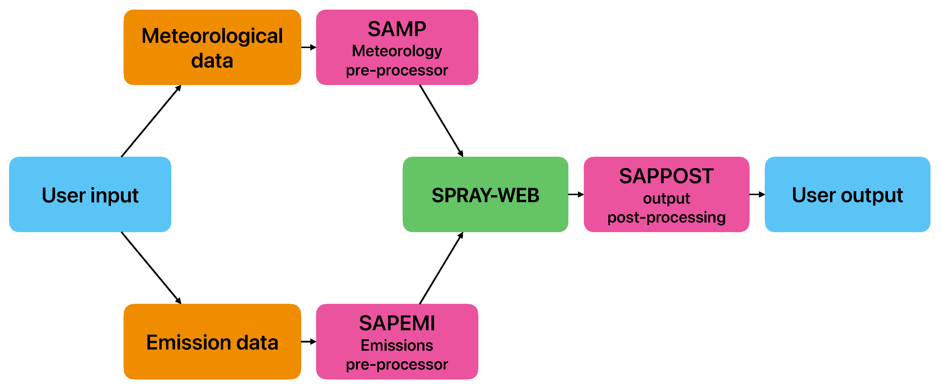
A flow chart representing the SAPERI modeling chain and its components is shown in Figure 1. Input data provided by the end user are the fire’s geographical location and its geometrical specification, the output concentration domain, the emission characterization and time evolution, the burning material type and quantity, and the simulation length. Part of this information is processed by the SAPERI emission pre-processor (SAPEMI) to build the pollutants release profile necessary for the dispersion model, SPRAY-WEB.

In parallel, meteorological data are retrieved for the selected domain and the turbulence fields are reconstructed through the SAPERI meteorological pre-processor (SAMP), which builds the external conditions file where the full meteorological time evolution is saved. Finally, the SAPERI post-processor (SAPPOST), starting from dispersion simulation output, produces georeferenced concentration maps providing quantitative spatial information and a statistical synthesis of the event impact on the selected domain.

2.1. Meteorological and Emissions Data Processing

In the default configuration, meteorological data are extracted from MISTRAL [21], the Italian meteorological open data portal providing data from various observation networks and different forecast products. Namely, the COSMO-2I dataset is used as the meteorological driver of choice. The forecast is produced by the COSMO meteorological model [20] in the framework of the LAMI agreement between the Italian Air Force Meteorological Service, the Arpae Emilia-Romagna Idro-Meteo-Clima Service and Arpa Piemonte, distributed under a CC BY-SA 4.0 license. The meteorological file is provided as a NetCDF and contains a 49 h forecast of the main three-dimensional variables, e.g., pressure, wind and temperature, on a grid with $2.2\mathrm{km}$ horizontal resolution and 15 vertical levels using a terrain-following coordinate system with a flat top at approximately $5\mathrm{km}$. It also contains some two-dimensional parameters, i.e.,  surface heat fluxes, surface roughness and land cover. Its coordinate reference system is the UTM (Universal Transverse Mercator) projection zone 32 over the whole territory.

In its default configuration, SAPERI includes a scheduler that runs continuously and downloads the most updated 00 run from the MISTRAL platform as soon as it is available. From the meteorological NetCDF file, the domain of interest for the emergency simulation can be cropped through the graphical user interface. In fact, for a private user, the open source downloading service does not allow to crop the domain upon request. In order to build a general purpose prototype, a pre-processing step was implemented in the SAPERI chain for cropping the original MISTRAL dataset. This step is not required in the case of an institutional user, making the tool faster and more efficient.

The SAMP pre-processor (Figure 1) computes the turbulent variables field through Hanna parametrization derived from scale analyses of the surface layer [25] on the selected domain. The friction velocity and the Monin–Obukhov length are calculated iteratively by applying the Monin–Obukhov similarity theory, the diurnal mixing layer height is computed following [26], while the nocturnal mixing layer height is the minimum value between the formulas suggested by [27,28]. The output of SAMP is used as meteorological input for the dispersion model SPRAY-WEB.

On the other hand, the SAPEMI pre-processor (Figure 1) produces the emission file serving as input for SPRAY-WEB, based on the information provided by the user. The emission time evolution is built from the date and time of the start of the pollutants release and of the foreseen conclusion of the accidental event. It is worth noting that the length of the emission period may not be equal to the length of the simulation. The emission profile is modulated according to an idealized initial ramp representing the initial development of the event. To simulate the gradual conclusion of the event, information or an estimate of the starting time of emergency services operations is also required. As illustrated in Figure 2, the combustion starts at time $t_0$ and the initial growth lasts until the full development of the fire at $t_1$; then the mass burned is constant until the firefighters intervention at $t_2$, while the final linear decay simulates the fire extinguishing phase at $t_3$. The trend shown in Figure 2 is simplified, exemplifying the evolution of an accidental event. The build-up of fire development spans two time steps. The emission stabilizes once the maximum power generated by the fire has been reached. This value is constrained by the total energy, computed from the calorific value and the total burned mass, for the specific time steps $t_0-t_3$.

All these parameters are set by the user. The descending ramp is a linear interpolation between the firefighters arrival time and the estimated end time of the event.

Additionally, SAPEMI estimates the buoyancy flux needed by SPRAY-WEB for each emission interval according to [29]; this computation requires knowledge of the fire geometrical size and the heat release rate. The latter is obtained from the total energy, retrieved from the total mass burned during the fire, its heating value, and the modulation profile described above.

Since the model is running in not-reactive mode, all emitted pollutants are proportional to the amount of burned mass. For the sake of efficiency, only one fictitious species is emitted and, according to the fire-specific emission factors, the concentration maps of all pollutants of interest are computed by the post-processing tool SAPPOST (Figure 1). A database with different emission factors from the current scientific literature is included in the tool, allowing the user to choose fire-specific defaults or to set custom values.

2.2. Dispersion Model and Post-Processing

SPRAY-WEB is chosen as the dispersion model at the core of the SAPERI modeling chain. As a Lagrangian particles model, it allows to obtain a high-resolution description of the plume rise dynamics since each particle interacts with the environmental conditions. The entrainment phenomenon depends on the temperature difference between the plume and the external environment and its modeling requires discretization with particles of the whole fluid, both plume and external air, which can result in a very large number of particles. In order to produce good statistics, a high number of particles is required and this leads to a high demand of computational resources in terms of both time and memory. To overcome this potential issue, the plume rise scheme proposed by [17] is used. This scheme involves a Lagrangian description in terms of the particle trajectories which transport the temperature difference $\Delta T_p$ and velocity information $v_p$. In addition, a Eulerian description is also involved, with the plume moving in a secondary grid characterized by the same information.

The steps describing the time evolution of the main parameters of the plume rise schema can be summarized as follows:

• Every time a particle emission occurs, $\Delta T_p$ and $v_p$ are initialized depending on the buoyancy flux and initial velocity computed by SAPEMI;
• Grid cell temperature differences and velocities ($\Delta T_c$ and $v_c$) are computed by summing the quantities transported by the particles inside it and normalizing for its volume;
• Grid cell quantities evolve accordingly with the equation proposed in [17];
• Particle $\Delta T_p$ and $v_p$ evolve in time on the basis of their position in the grid and the cell quantities.

This procedure is repeated every plume synchronization time step ($d{t}_{pr}$), which can be different from the particles advancement time step ($dt$) and from the particle emission time step ($d{t}_{emi}$). In the default setup, it holds that $d{t}_{emi}=d{t}_{pr}\ge 5\ast dt$. Sensitivity analysis (not shown) suggests that the quality of results is preserved while varying the plume rise computation time step, the number of emitted particles and the plume rise Eulerian grid; this warrants the assertion that this plume rise scheme is sufficiently robust. Then, the optimal configuration of these parameters is chosen by following the maximum performance criterion to obtain the desirable execution speed.

The output ground concentration fields for the pollutants requested by the user are computed by SAPPOST. The concentrations are retrieved from the proxy species simulated using the emission factor specific for the material burning in the event for each pollutant. For each species involved, its impact on the domain is represented by a map showing the maximum ground level concentrations reached during the entire event. Additionally, the footprint map is calculated according to the following definition:

$$f(x,y)=\left\{\begin{array}{cc}1,\hfill & \mathrm{if}c(x,y)>c_{\mathrm{threshold}}\hfill \\ 0,\hfill & \mathrm{otherwise}\hfill \end{array}\right.$$

(1)

where $f(x,y)$ is the footprint at point $(x,y)$, $c(x,y)$ is the concentration and $c_{\mathrm{threshold}}$ is $5\%$ of the $98\mathrm{th}$ percentile of the maximum field non-null values distribution. The maximum concentration field gives quantitative information about the peak concentration during the simulation, while the footprint map is designed to provide qualitative information about the extension of the areas affected by the dispersion of pollutants.

2.3. Parallelization

Lagrangian particle models are able to achieve a high degree of accuracy by tracking the trajectories of individual particles; however, this precision implies a significant computational cost, since it is required to emit a large number of particles. In emergency situations, obtaining results as quickly as possible is crucial; therefore, it is required to reduce the computational time of the SPRAY-WEB dispersion model as much as possible. We implemented a strategy to parallelize the code on a general purpose graphical processing unit (GPU) with the high-level programming framework OpenACC.

SPRAY-WEB is written in Fortran and features a time loop that spans the duration of the simulation. This loop involves the emission of new particles and the transport and dispersion of existing particles within the domain at each time step. Parallelization allows to accelerate the particle loop, where particles evolve independently of one another, by distributing the computations across multiple threads. These threads progress simultaneously, exploiting the large number of cores of the GPU to significantly speed up the process. As an example, the OpenACC directive to accelerate the particles’ loop is as follows:

!$acc parallel loop gang vector num_gangs(nblocks) vector_length(nthreads)

This directive tells the compiler to distribute the iterations of the loop among the number of threads specified by nblocks, nthreads, so that each thread processes multiple particles.

As the simulation progresses, the number of particles to be included in the parallelization loop increases, and the data transfer from the host to the GPU becomes increasingly heavy. For this reason, we aimed to perform as much computation as possible directly on the GPU, limiting data transfers to only what is strictly necessary, specifically when new meteorological data must be read and when output files need to be written. It is worth noting that the parallelization of the plume rise algorithm [17] required particular care, due to the mixing of Lagrangian and Eulerian approaches.

One of the most challenging tasks in the context of code parallelization is the generation of pseudo-random number series. These are essential for the stochastic evolution of particle trajectories. To achieve this from a single seed, we initialized a series of initial states with a length of nthreads*nblocks. Each state is then used to generate a series of pseudo-random numbers using NVIDIA’s curand_init function.

To take advantage of the parallelization, the end user has to run the model on a machine equipped with a general purpose GPU, either locally or remotely. The results described in the following section were achieved with an NVIDIA Tesla T4 GPU and each simulation run, spanning 49 h, took about 20 min. Details of the parallelization strategies, including performance analysis in comparison with the traditional sequential code, will be provided in a separate paper.

3. Results

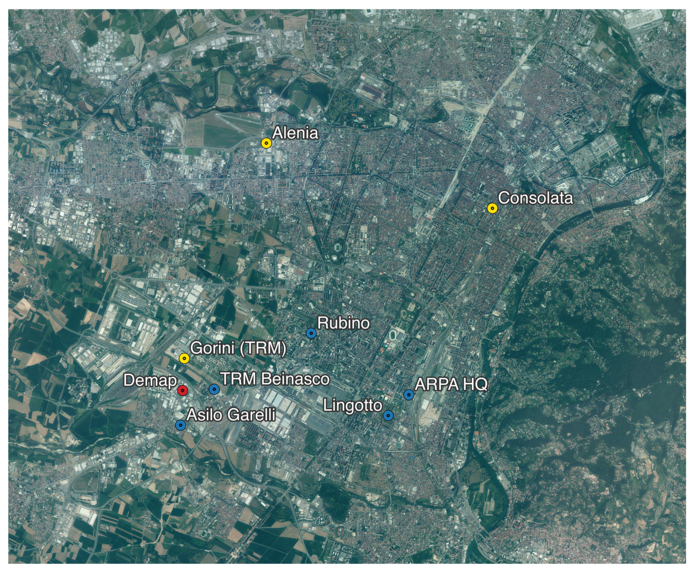
In this section, we show an application of the SAPERI modeling chain to a real case—an industrial fire which occurred at a plastic waste facility in Beinasco (Torino, Italy) on 12 December 2021 (see Figure 3). The SAPERI modeling chain was configured to simulate a real case emergency management scenario characterized by inherent uncertainties in the event definition. Setting up an emergency numerical simulation is challenging due to the limited initial data availability and the urgency to alert the potentially affected nearby population and to support first-responders. Meteorological forecasts may have coarse spatial resolution and may not accurately capture the local patterns, thus influencing prediction of the plume dispersion. Furthermore, limited or no information is usually available about the total mass of the burning material, its precise composition, or its physical state (humidity, temperature, etc.). The spatial extent of the fire might also be unknown. In order to evaluate the potential efficacy of the tool in supporting decision-makers during emergency response in the designated case study, we compared the results of SAPERI with observations collected by meteorological and air quality monitoring stations, fixed and mobile, later made available.

According to the assessment report written in the months following the event by local authorities (the Piemonte Region Environment Protection Agency, ARPA) [30], the fire event started at 15:30 on 12 December 2021 and lasted for more than two days. The acute event was followed by a phase with extinguished flames yet with persistent release of hazardous airborne pollutants. As if in the real emergency situation, we carried out new dispersion simulations as soon as new up to date weather forecasts from the COSMO-2I model were available on the MISTRAL portal. Four different model simulations were run with distinct meteorological input spanning the period from December 12 to 17, overlapped by 24 h. The model domain is centered on the incident site and it has a size of 28.6 km in each horizontal dimension. The top of the domain is at 4900 m, because in case of industrial fire, the plume usually remains under 4900 m and cropping the meteorological file at this height helps in saving time and space, but this setting can be changed if necessary in a specific installation. The simulation time step is set to 2 s while the emission source characterization step is 30 min.

The combustion of plastic releases multiple hazardous species into the atmosphere, including particulate matter, ammonia, carbon monoxide and VOCs among others, as well as persistent organic pollutants, such as polycyclic aromatic hydrocarbons and dioxins and dioxin-related compounds [31]. In the following analysis, we will focus on benzene and dioxins (PCDD/DFs). The first is routinely measured by fixed air quality stations, being one of the key pollutants targeted by the European Air Quality policy; the latter are usually monitored during fire events, both in terms of air concentrations and ground depositions, since they can easily pose a serious health risk by entering into the food chain. In the total absence of data useful to characterize a realistic emission source term, such as the amount of plastic wastes stored in the plant when the fire occurred, input parameters were derived from regulatory authorizations issued by local authorities [32,33]. The energy release was estimated at $5.1\times {10}^7\mathrm{MJ}$, calculated by multiplying the heating value of polyethylene terephthalate (PET) $3.4\times {10}^7\mathrm{J}{\mathrm{kg}}^{-1}$ [34] by the total mass of burning plastic waste, roughly estimated at $2\times {10}^6\mathrm{kg}$. The emission factor for benzene was selected at $0.9\mathrm{g}{\mathrm{kg}}^{-1}$ waste burned [35], while the dioxins PCCD/F emission factor was set at $1.22\times {10}^{-7}$ g (TEQs) ${\mathrm{kg}}^{-1}$ waste burned, retrieved from the same reference. The burning area diameter was set to 65 m, based on aerial photographs of the facility.

The emission temporal profile was built by modifying the standard modulation represented in Figure 2 to account for the prolonged duration of the event, lasting multiple days. As previously reported, the fire started at 15:30 on December 12 ($t_0$). The acute phase plateau, with maximum emission, lasted one hour from 16:00 ($t_1$) to 17:00 ($t_2$) of the same day, when the firefighters arrived at the site [30]. The emission rate at the tail of the final slope was adjusted to be constant with a non-zero value.

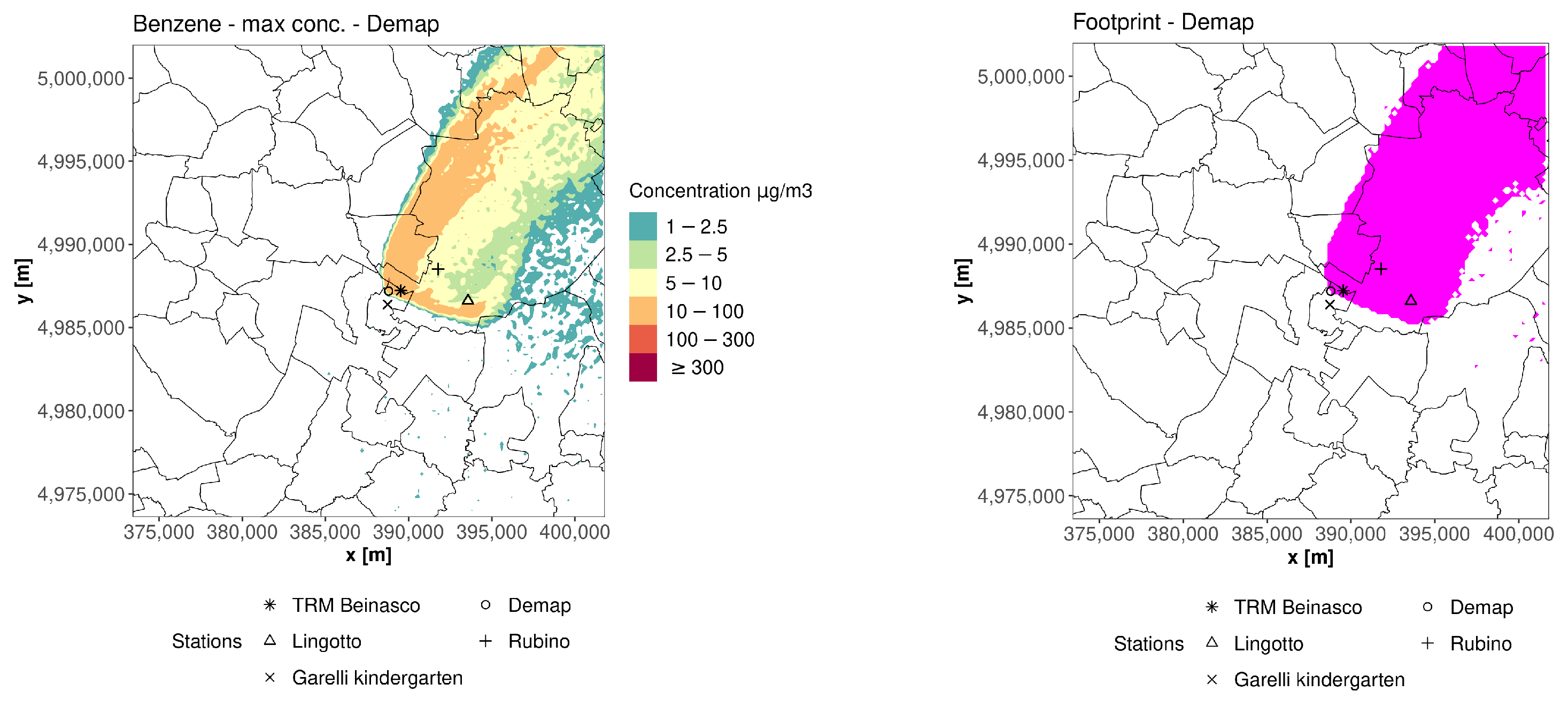
Figure 4 shows the typical outputs of the SAPERI modeling chain for the first simulation run corresponding to 12–14 December. On the left, a map of the maximum ground level concentration of benzene is presented (concentrations expressed as $\mathsf{\mu }\mathrm{g}{\mathrm{m}}^{-3}$), while on the right, the event footprint is shown.

The maximum concentration map provides a preliminary quantitative assessment of the impact of the incident on nearby areas, though it is affected by the already mentioned incomplete details about the incident. Conversely, the qualitative information delivered by the footprint is only partially affected by the uncertainties of the numerical simulation setup, since it is independent of the specific emission factor. Furthermore, from the first-responders’ point of view, it immediately highlights the extension of the affected area and it provides support to alert nearby populations. In this case study, the plume propagates towards the north-east direction directly impacting the whole Torino urban area. These maps also identify the air quality stations impinged by the plume (colored dots), which will be used to perform the following numerical comparisons.

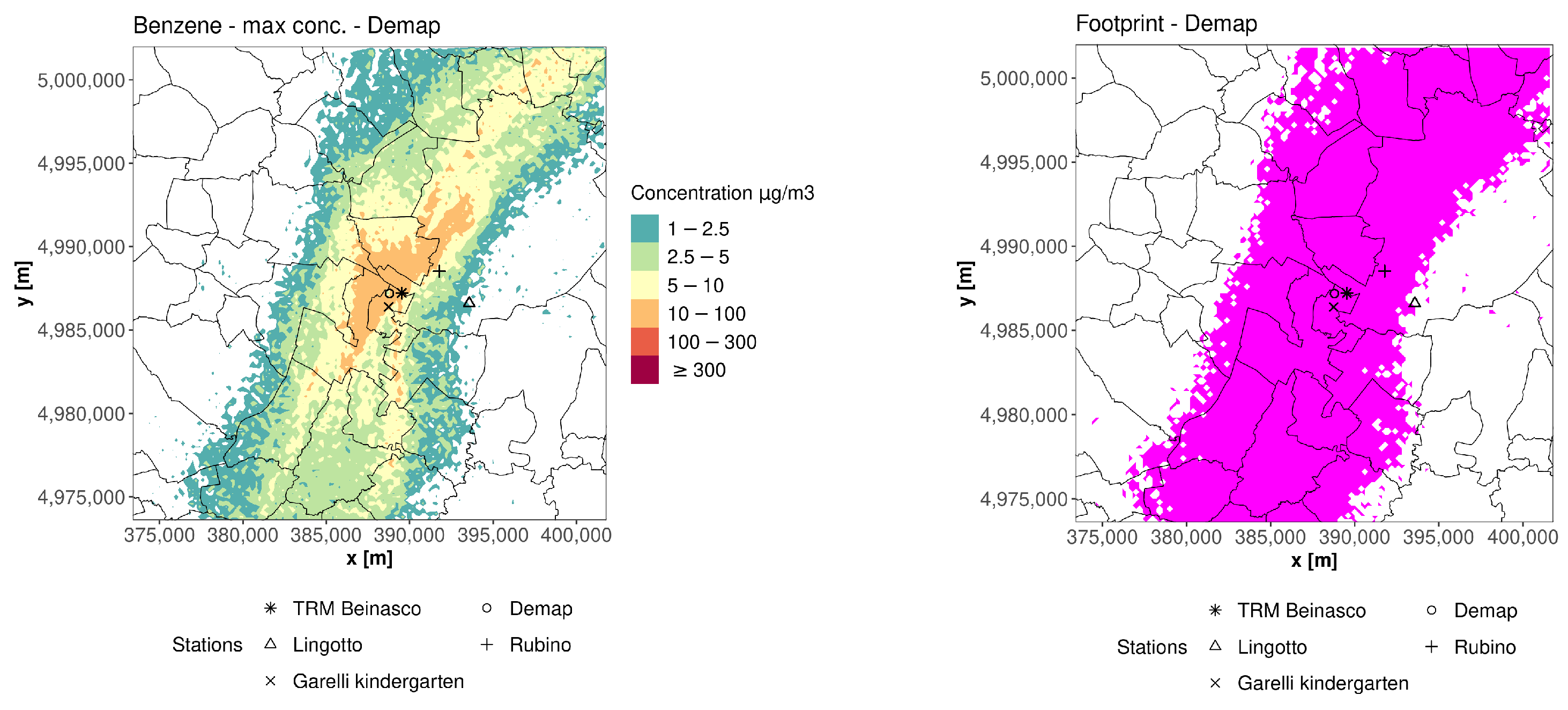
In Figure 5, Figure 6 and Figure 7, the SAPERI outputs for the three additional runs are presented. Both the maximum ground level concentration and the footprint maps show how the plume fallout evolves in time, impacting also the areas south-west of the plant. From the maximum concentration maps, it can also be noted that the extension of the region with higher levels of benzene concentration reduces over time and remains closer to the source location.

In order to evaluate the performance of the SAPERI modeling chain for the case study, a comparison analysis was performed with measurements available from meteorological and air quality monitoring stations. The comparison analysis also provides some insight into the uncertainties related to the absence of information about the source term.

3.1. Meteorological Simulations

A preliminary analysis of the meteorological input of the dispersion model was performed by comparing the modeled data and observed measurements retrieved from three stations, Torino via della Consolata, Torino Alenia and Gorini (see Figure 3), from the Regione Piemonte monitoring network. We compared hourly values of temperature, wind speed and wind direction with the values extracted from the COSMO-2I forecasts at the same location of the stations. The model temperature and wind were extracted at vertical levels of 2 m and 20 m. 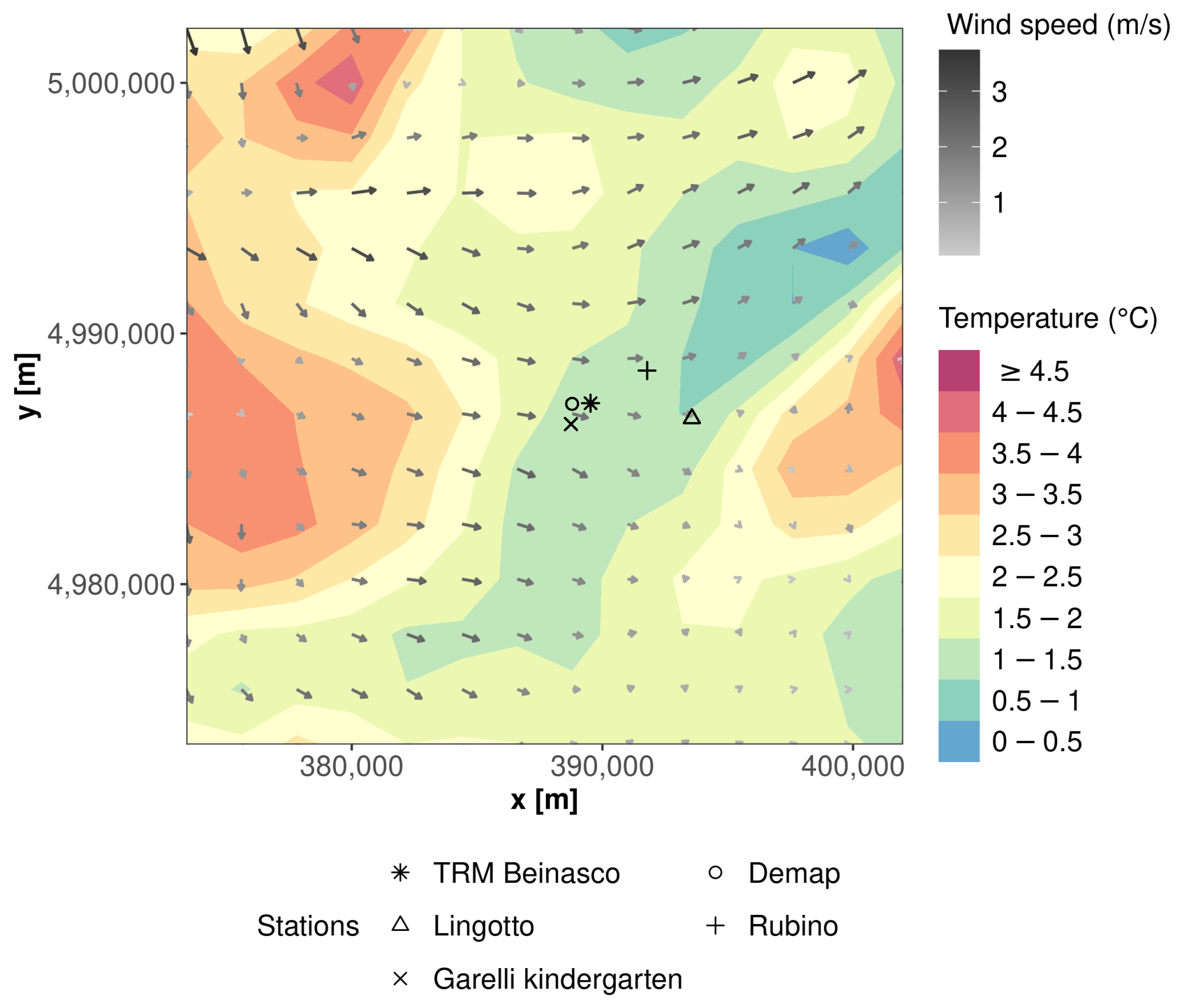In Figure 8, an example of the wind and temperature fields is shown.

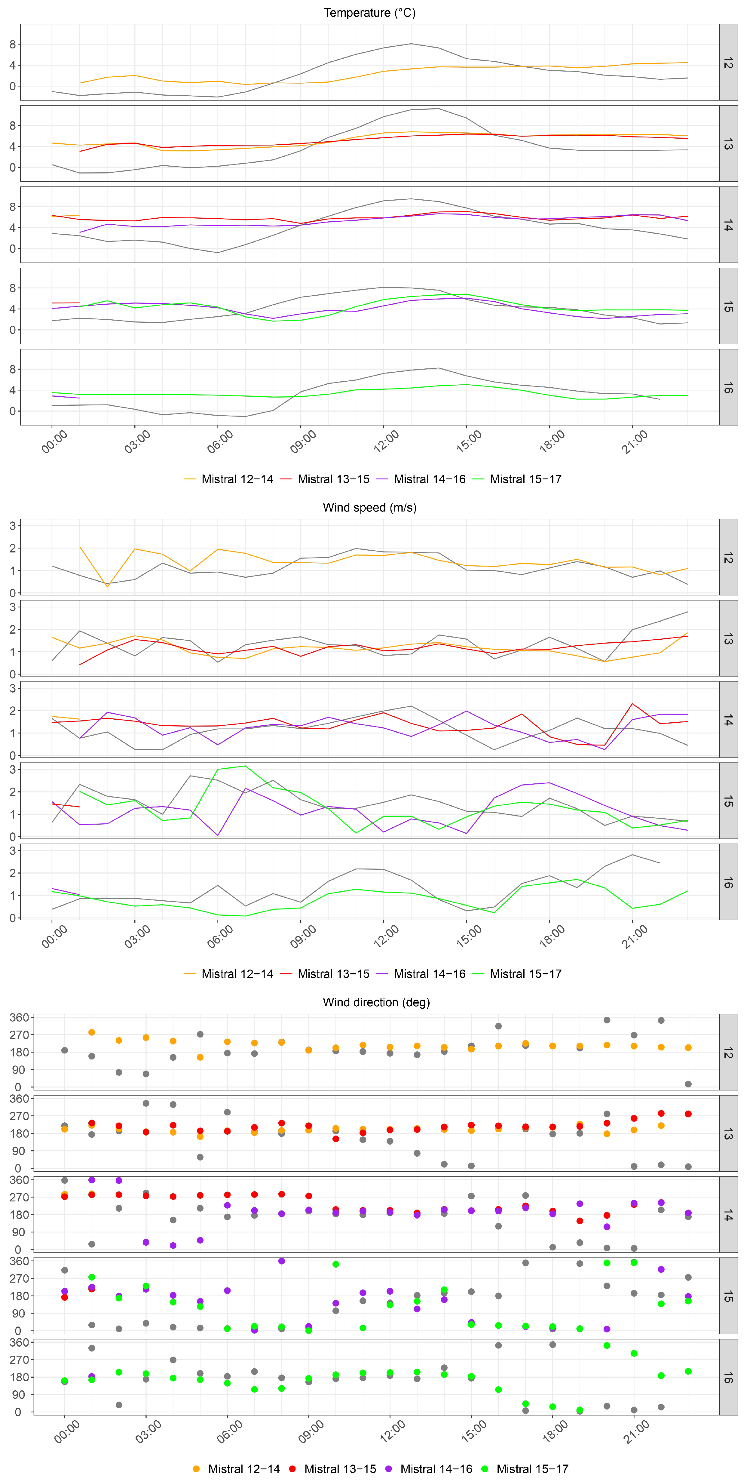
The results of the comparison for each station are presented in Figure 9, Figure 10 and Figure 11, respectively. In each figure, the rows correspond to a different day of the event, from the $12\mathrm{th}$ (top) to the $16\mathrm{th}$ (bottom). Grey lines and dots represent the measured values while colored lines and dots represent the COSMO-2I forecasts, with each color corresponding to a different model run.

Table 1. Statistical indices for temperature, wind speed and wind direction, comparing COSMO-2I forecasts with observations at three meteorological stations.

	Torino Alenia	Torino Consolata	TRM-Gorini
	Temperature
NMSE	0.22	0.47	0.26
FB	$-0.07$	0.2	$-0.27$
FAC2	0.82	0.67	0.8
R	0.69	0.63	0.67
	Wind speed
NMSE	0.29	0.33	0.4
FB	$-0.17$	$-0.07$	0.17
FAC2	0.76	0.72	0.69
R	0.36	0.21	0.22
	Wind direction
NMSE	0.28	0.51	0.48
FB	$-0.12$	0.13	0.22
FAC2	0.78	0.71	0.55
R	0.32	0.06	0.28

reports a statistical evaluation of the meteorological data through four statistical indices defined as follows, where P are the predicted values and O are the observed values:

• Normalized mean squared error (NMSE):

  $$NMSE=\sqrt{\overline{{(O-P)}^2}}$$

  (2)
• Fractional bias (FB):

  $$FB={\displaystyle \frac{\overline{P}-\overline{O}}{0.5\times (\overline{P}-\overline{O})}}$$

  (3)
• Factor of two (FAC2)

  $$FAC2={\displaystyle \frac{\Sigma (R>0.5\wedge R<2)}{length\left(R\right)}}$$

  (4)

  where $R={\displaystyle \frac{P}{O}}$.
• Pearson correlation coefficient (R)

The statistical analysis was performed by considering the temporal series of the meteorological parameters corresponding to the most updated values available, i.e., the first 24 h of each 49 h COSMO-2I forecast.

In general, the temperature from the model forecasts exhibits a flatter trend compared to observed data at the monitoring stations, while conserving a quite good correlation. Wind speed presents low absolute values both for the forecasts and the observations. Model values accurately reproduce measurements for the Alenia station (Figure 10), while they are slightly overestimated for the two other stations. As for wind direction, some discrepancies between the forecasts and the observations emerge, mainly for Torino Consolata that is located in the city center. Since the model does not take urban canopy effects into account, the correlation coefficient for direction is not satisfactory. However, the other indices are suitable for a screening application.

3.2. Air Quality Simulations

Air quality comparison between model output and observed data was performed at three monitoring stations: Beinasco Aldo Mei (TRM), Torino Rubino e Torino Lingotto (see Figure 3), and from the Regione Piemonte monitoring network.

Before proceeding, we applied a mitigation procedure to take into account the wind direction discrepancies that emerged in the previous analysis. The wind direction uncertainty was estimated as twice the mean absolute error (MAE) computed at the nearest station to the fire site, i.e., TRM-Gorini, with MAE defined as:

$$\mathrm{MAE}={\displaystyle \frac{{\sum }_{i=1}^n(p_i-o_i)}{n}}$$

(5)

where n is the number of observations, $p_i$ is the predicted value and $o_i$ is the observed value. The computation was repeated for each simulation run, corresponding to four distinct meteorological forecasts (see

Table 2. Mean absolute error (MAE) and corresponding uncertainty angle for wind direction for each meteorological forecast.

Day	COSMO-2I Run	MAE	Uncertainty ($\mathit{\alpha }$)
12 December 2021	12–14 December	57°	114°
13 December 2021	13–15 December	67°	134°
14 December 2021	14–16 December	57°	114°
15 December 2021	15–17 December	64°	128°

). Given the wind direction uncertainty, a circle arc centered on the fire site was defined with length $l=d·\alpha$ with radius d equal to the distance to each air quality station and with angle $\alpha$ defined as in Table 2 (expressed in radians).

The concentration along the arcs was sampled every 3° and the maximum value was chosen to be compared with the air quality measurements.

Despite being a good tracer for plastic burning, measured benzene is affected by emissions originating from other sources, mainly vehicular traffic. For this reason, at each station, we estimated an hourly modulated background concentration by considering “by hour” means of the winter season levels (December, January and February) for years 2018 and 2019. In the quantile–quantile plots (Figure 12), the observed and simulated concentrations, paired from the smaller to the greater, are compared after removing the background. They represent a comparison of the observed and simulated distributions. Although the modeled concentrations overestimate the observations, there is a clear correlation between the data and the corresponding best-fit straight line is plotted in red. Some observed concentrations are matched by zero modeled ones; this is probably due to the background estimation methodology. The overestimation could be attributed to the simplified source characterization and to the uncertainties related to the benzene emission factor for plastic burning. As a consequence, we applied a correction based on the linear regression of the qq-plots (Figure 12). In particular, model outputs were rescaled by multiplying each value by the angular coefficient and by summing the intercept as computed from the best fit (red lines in the figures).

This methodology provides a rescaled concentration, keeping unaltered the relative magnitude of the model outputs, independently of the temporal evolution, and it is useful to evaluate the model’s capability to capture the concentration peak events.

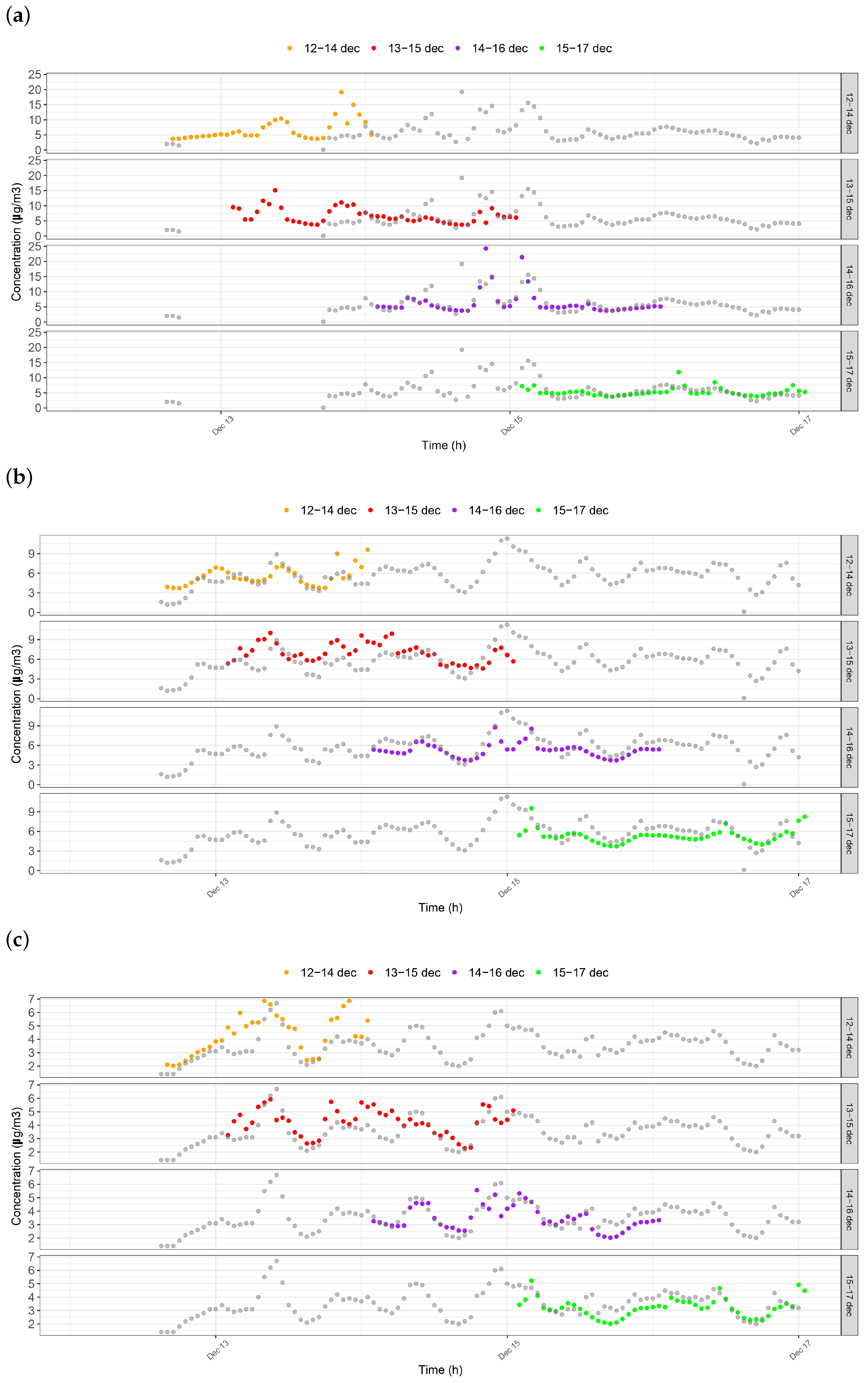
Figure 13 shows a comparison between the hourly values measured by the monitoring stations and the model output, rescaled as described above and with the addition of the modulated background values. Each panel corresponds to a monitoring station and each row within the panel corresponds to a distinct simulation run. Model output is represented by colored dots and the observed values by grey dots.

Beinasco (TRM)-Aldo Mei (Figure 13a) is the nearest station to the fire site but, unfortunately, it was shut down for a few hours right after the fire broke out due to a power-line shortage directly related to the emergency itself [30]. The time series illustrate that the model well reproduces the peaks in the observations, especially the two events between December $14$ and $15$. The Torino-Lingotto station (Figure 13b) is slightly laterally shifted with respect to the plume direction, but it still well reproduces, especially, the high concentration level measured between December $14$ and $15$, even if it is split in two peaks. Also at the Torino-Rubino station (Figure 13c), the model output series correctly identify the peak of December $13$.

Figure 14 presents the scatter plots at the three stations and it confirms that the SAPERI modeling chain is capable to reproduce the observed peaks in the monitoring data. After rescaling, most of the data points lay within a factor of two of the observations. As suggested by the concentration time series, we obtained the best results for the Torino-Rubino station. This analysis confirms that the discrepancies between the measured values and the model output are mainly due to the uncertainties related to the simplified source characterization and to the specific emission factor.

Additional analysis was performed by considering the dioxins concentrations at the critical receptor Garelli kindergarten in Beinasco (see Figure 3), where a mobile monitoring device was placed several hours after the alarm was given. Dioxins, similarly to benzene, can be considered a typical tracer of uncontrolled plastic combustion, while their measured values are less affected by the contribution of other potential sources, such as vehicular traffic [30]. Considering the meteorological forecast, at the beginning of the event, the measuring station remained downwind of the event location for just a few hours, while for most of the time, the wind blew in the opposite direction. This can introduce some errors in the evaluation of the concentration levels; therefore, in the comparison, we considered the maximum values at the distance between the fire site and the measuring station, regardless of direction.

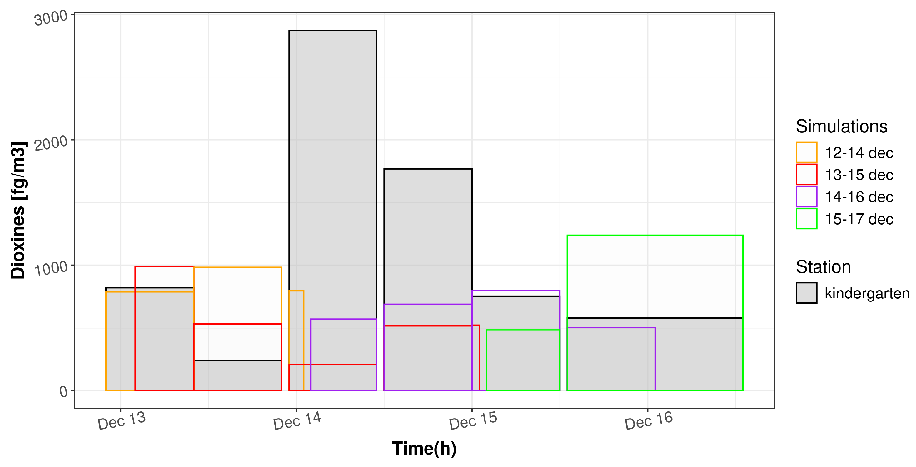
In Figure 15, the measured data are compared with the model output. The bin width represents the length of the time sampling average—12 h for the first days and then 24 h. The grey shaded columns correspond to the measured data, while the columns with colored borders represent the values estimated from the four different simulations after adding a constant background value to the model output, computed by taking the mean values measured in December for the years 2018 and 2019 at the Beinasco (TRM)-Aldo Mei station.

The comparison between the measured and simulated values suggests that the model correctly reproduces the order of magnitude of the dioxin concentration. This means that an early warning system, such as the SAPERI modeling chain, even in the case of uncertain weather forecast, can provide immediate information on the maximum expected air pollution level and the amount of people potentially affected.

ARPA Piemonte also conducted dioxin sampling for 12 h at its headquarters on the night between December $12$ and $13$, as the wind direction suggested a plume fallout in that area (see Figure 3). In this case, since the forecast wind direction was favorable, as suggested by the footprint map in Figure 4, the comparison was directly conducted with the model output extracted at the exact location of the sampling. The measured value was $80\mathrm{fg}\mathrm{I}-\mathrm{TEQ}{\mathrm{m}}^{-3}$, while the model estimation from the first simulation run is $92\mathrm{fg}\mathrm{I}-\mathrm{TEQ}{\mathrm{m}}^{-3}$, showing good agreement between the values.

Both results for the dioxins comparison suggest that, in this case study, the emission factor selected for the analysis is suitable to obtain accurate quantitative results.

4. Conclusions

In this paper, we presented the SAPERI modeling chain, developed to provide forecast information in the case of an accidental release of airborne pollutants in emergency situations, such as in the case of an industrial fire. The tool can be used by emergency operators in the immediate aftermath of the onset of an incident and replicated during its development, given its ease of use and its execution speed. It is also possible to reconstruct past incidents, overriding default parameters with more detailed information about the event. Acceleration through a general purpose GPU, implemented with OpenACC, delivers fast execution of the Lagrangian three-dimensional dispersion model SPRAY-WEB, at the core of the modeling chain. Sensitivity analysis and fine tuning of the dispersion model parameters also enabled further reduction in the computational time, preserving good quality of results.

The impact maps produced by SAPERI highlight the extension of the affected areas though they do not have a toxicological characterization and are meant to mainly provide qualitative information to emergency responders. A real case scenario (Beinasco, 2021) was presented. The lack of knowledge about the source characterization and the adoption of a forecast meteorological input with $2.2\mathrm{km}$ horizontal resolution limits the accuracy of the results. In order to compare the simulation results with observations obtained at the institutional monitoring network and to assess the modeling chain performance, the robustness of the selected emission factors, and the accuracy of the algorithms employed to simulate plume rise and dispersion, we applied some post-processing techniques to mitigate the effects of the input uncertainties.

The results here presented show that the SAPERI modeling chain has the capability to simulate complex situations in emergency conditions. In particular, we found that the meteorological input from COSMO-2I is in good agreement with the observations, although some discrepancies emerged for wind direction. In order to be employed as an operational early warning system, SAPERI may benefit from meteorological fields downscaling, especially in complex terrain. As far as the source characterization is concerned, the emission factor selected for benzene underestimates the magnitude of the concentration levels, while for dioxins, the results are satisfactory, even from a quantitative point of view. The dispersion model is capable to predict the temporal evolution of the phenomenon, correctly identifying the main concentration peaks, thus providing useful information for first-responders and local authorities.

In the framework of commercially or freely available early warning systems, SAPERI is suitable for a wider spectrum of potential end users thanks to its ease of deployment and configuration, limited amount of required information, cost-effective use of computational resources, and flexibility in the choice of meteorological input. Compared to the tools already available, it introduces an innovative plume rise scheme for fires based on the buoyancy flux, which makes it especially appropriate for simulating industrial fire-type emergencies. By comparing the obtained results with observations in a real case, we can conclude that the prediction accuracy of the system is satisfactory. In the future, a more in-depth study will be carried out on the emission profile modulation during the ignition and extinguishing phases of the fire, with a special focus on smouldering currently not considered. Further development in the field of forest fires is underway.