Article

Analysis of Global and Key PM2.5 Dynamic Mode Decomposition Based on the Koopman Method

by
Yuhan Yu
1,
Dantong Liu
1,
Bin Wang
1 and
Feng Zhang
1,2,*
1
School of Earth Sciences, Zhejiang University, Hangzhou 310027, China
2
Zhejiang Provincial Key Laboratory of Geographic Information Science, Hangzhou 310027, China
*
Author to whom correspondence should be addressed.
Atmosphere 2024, 15(9), 1091; https://doi.org/10.3390/atmos15091091
Submission received: 2 August 2024 / Revised: 25 August 2024 / Accepted: 3 September 2024 / Published: 8 September 2024
(This article belongs to the Section Air Quality)

Abstract

:
Understanding the spatiotemporal dynamics of atmospheric PM2.5 concentration is highly challenging due to its evolution processes have complex and nonlinear patterns. Traditional mode decomposition methods struggle to accurately capture the mode features of PM2.5 concentrations. In this study, we utilized the global linearization capabilities of the Koopman method to analyze the hourly and daily spatiotemporal processes of PM2.5 concentration in the Beijing–Tianjin–Hebei (BTH) region from 2019 to 2021. This approach decomposes the data into the superposition of different spatial modes, revealing their hierarchical spatiotemporal structure and reconstructing the dynamic processes. The results show that PM2.5 concentrations exhibit high-frequency cycles of 12 and 24 h, as well as low-frequency cycles of 124 and 353 days, while also revealing spatiotemporal modes of growth, recession, and oscillation. The superposition of these modes enables the reconstruction of spatiotemporal dynamics with a mean absolute percentage error (MAPE) of only 0.6%. Unlike empirical mode decomposition (EMD), Koopman mode decomposition (KMD) method avoids mode aliasing and provides a clearer identification of global and key modes compared to wavelet analysis. These findings underscore the effectiveness of KMD method in analyzing and reconstructing the spatiotemporal dynamics of PM2.5 concentration, offering new insights into the understanding and reconstruction of other complex spatiotemporal phenomena.

1. Introduction

PM2.5 is a critical indicator of air pollution, with serious implications for human health, contributing to approximately 4.2 million deaths worldwide each year [1]. The variations in PM2.5 concentrations show distinct patterns that combine both cyclic and non-cyclic spatial distributions [2,3]. This complexity poses a great challenge in interpreting and predicting the spatial and temporal processes of PM2.5 concentration.
To explore the dynamic spatiotemporal patterns of PM2.5 pollution, researchers have employed various modeling methods, including the Community Multiscale Air Quality (CMAQ) method [4], Dynamic Mode Decomposition (DMD) [5], Principal Component Analysis (PCA) [6], wavelet analysis [7], and Fourier decomposition [8], to reveal the spatiotemporal structural characteristics of PM2.5. However, the DMD method is notably noise-sensitive, which can lead to errors in mode identification. On the other hand, PCA effectively identifies patterns in data by projecting them onto an optimal subspace but often overlooks the temporal characteristics of the data. Fourier decomposition may result in a loss of phase information, while the Empirical Mode Decomposition (EMD) method excels at analyzing non-stationary data series [8,9]. However, the EMD method encounters challenges with mode mixing, where high- and low-frequency modes can overlap and interfere during analysis. The boundary effects of the wavelet transform, when dealing with signals of finite length, can lead to inaccurate signal transform results [10]. To enhance analysis, Ensemble Empirical Mode Decomposition (EEMD) has been utilized to break down PM2.5 time series data [11,12]. However, the EEMD method often struggles with issues like residual white noise, and the selection of effective mode functions depends significantly on analyst expertise, which can affect the precision of both decomposition and reconstruction. Consequently, there is a pressing need for an approach that can approximately, efficiently, and accurately decompose hierarchical patterns, which is essential for a comprehensive understanding of the global characteristics of complex systems and an effective response to nonlinear data.
The Koopman Mode Decomposition (KMD) method is an advanced analytical technique grounded in the Koopman operator theory, designed to study nonlinear dynamic systems. The KMD method works by decomposing observed data from a system, thereby revealing its various frequency components and capturing both local and global dynamics. A significant advantage of this method lies in its ability to provide global linearized representation through the Koopman operator, which simplifies the analysis and enhances the understanding of complex systems. This approach also accurately captures the system evolution within the state space. Unlike methods that rely on specific dynamic equations, the KMD method directly extracts the dominant dynamic modes from experimental or simulation data, uncovering the system’s underlying structure and behavior. Therefore, the Koopman method offers distinct advantages in analyzing and predicting complex nonlinear dynamic systems, offering fresh perspectives and powerful tools for tackling challenges in spatiotemporal processes.
The Koopman method has been successfully applied in a variety of fields such as transportation [13,14], healthcare [15,16], flow [17,18], and control systems [19,20,21]. For example, Ling [22] developed a method based on Koopman operator theory and Dynamic Mode Decomposition (DMD), applying it to the analysis and control of signalized traffic flow networks, thereby demonstrating its effectiveness in practical traffic management. Kim [15] introduced a Compatible Window-wise Dynamic Mode Decomposition (CwDMD) approach for analyzing the spatiotemporal transmission patterns of COVID-19, offering valuable insights for public health management. Mezić [18] explored Koopman modes and revealed that the theory provides a unified theoretical framework for global modal analysis, triple decomposition, and the DMD, thus enabling the efficient analysis and control of traffic flow networks. Bruder [20] proposed a method based on Koopman operator theory for the system identification and control of soft-bodied robots, demonstrating its utility in the control of real soft-bodied robots. These applications highlight the universality and efficacy of Koopman operator theory in various systems, offering innovative tools and perspectives for solving practical challenges. However, the effectiveness of the KMD method is contingent on data quality. If the data are noisy or the observation period is brief, the method’s ability to accurately capture the system’s true dynamic patterns may be compromised [23]. Furthermore, when applied to large-scale datasets or high-dimensional systems, the KMD method may struggle to accurately capture all dynamic features, potentially impacting the reliability of the results.
In this study, we apply the KMD method to analyze PM2.5 concentrations across 76 monitoring stations in the Beijing–Tianjin–Hebei (BTH) region, utilizing hourly and daily average data from 2019 to 2021. Our objective is to reveal the underlying spatiotemporal dynamics and accurately reconstruct these processes. To assess the accuracy and effectiveness of the KMD method in analyzing the spatiotemporal patterns of PM2.5 pollution, we compare our findings with those obtained from the EMD method and wavelet analysis. Furthermore, this study introduces a novel tool for understanding and reconstructing other complex spatiotemporal phenomena.

2. Materials and Methods

2.1. Materials

2.1.1. Study Area

Figure 1 shows the BTH region, located in the northern part of the North China Plain. By 2021, the BTH region’s GDP had grown to approximately 2.2 trillion USD, constituting about 10.6% of China’s total GDP. According to the Report on the State of the Ecology and Environment in China, the annual average PM2.5 concentration in the BTH region was 64 μg/m3 in 2017. This level is significantly above the World Health Organization (WHO)’s air quality standard of 35 μg/m3, making it one of the most severely polluted areas [24,25]. Therefore, understanding and reconstructing the spatiotemporal processes of PM2.5 pollution in the BTH region can enhance air quality management in the area and serve as a valuable reference for air pollution prevention and control in other regions.

2.1.2. Data Sources

Hourly PM2.5 concentration data for the BTH region from January 2019 to December 2021 were sourced from the China National Environmental Monitoring Centre (CNEMC, http://www.cnemc.cn/ (accessed on 5 September 2024). Data were collected from 234 monitoring stations located at the BTH. All data were verified automatically and manually and processed as follows: (1) the monitoring stations of suspension operation were removed; (2) stations that were empty for 12 consecutive hours in a day were also removed; and (3) when calculating monthly averages, the data coverage for a given month could not be less than 28 days, otherwise the data were invalidated and removed. Therefore, we used the mean-imputation method to complete the missing data for PM2.5 over 12 consecutive hours [26]. The percentage of missing values was approximately 1.7%. Ultimately, we identified 76 monitoring stations for this study (Figure 1).
Based on the new Air Quality Guidelines (AQGs) released by the World Health Organization (WHO) [27], we conducted an uncertainty assessment on the PM2.5 dataset processed using the mean-imputation method. We used the first 500 h of data from January 2019 at the first monitoring station as an example, randomly removing 10% of the data to create an artificial validation set that simulated missing values [28]. The missing values were then filled using the mean-imputation method, and the errors and uncertainties between the interpolated results and the original data were subsequently calculated. The results indicated that the root mean square error (RMSE) between the interpolated data and the original data was 1.83, the mean bias error (MBE) [29] was 0.02, and the En value [29] was 0.1%. These findings indicate that the relative uncertainty of the interpolated data is minimal compared to the original data, thereby confirming the feasibility and effectiveness of the mean-imputation method for addressing missing data.

2.2. Koopman Operator

2.2.1. Definition of Koopman Operator

The Koopman operator, proposed by B O. Koopman, in the evolution of state functions in Hilbert space provides a unique way to describe dynamic systems [30,31]. The operator  K  is inherently infinite-dimensional and linear, but it can be approximated by a finite-dimensional  K -matrix. This approximation facilitates the observation of nonlinear system evolution within a finite space. The detailed formulas are as follows:
x t + 1 = f x t ,   x t M ,
The variable  x t  represents a point in the state space  M , which denotes the system state at time step  t . The function  f  represents the mapping from one state to another within the state space  M .
K  represents the evolution of one of the Koopman linear operators describing the any observable function  g  on phase space orbitals. For any observable function  g   : M C .
K g x t = g f x t ,   g   : M C ,
C  denotes the set of complex numbers, indicating that the function  g  maps points from the state space  M  to the complex domain  C .
The Koopman operator has following dynamics:
K φ x t = φ f x t = λ t φ x t .
φ  is the eigenfunction of the Koopman operator, also referred to as the observation function, which maps the system state to a new function space. In this new space, the action of the Koopman operator  K  is linear.  λ  denotes the eigenvalue of the Koopman operator, which characterizes the dynamic behavior of the eigenfunction  φ f x t  represents the nonlinear dynamic mapping of the system, indicating the transition from the state  x t  to  x t + 1 . Koopman eigenvalues and eigenfunctions capture the overall dynamics of a system, including essential characteristics like periodicity, growth, and decay [32,33,34].
The real part of an eigenvalue  λ  represents the growth or decay rate of the mode, while the imaginary part is used to compute the oscillation period of the mode [13]. In the complex plane, the unit circle is composed of all complex numbers with a modulus of 1. The modulus of an eigenvalue  λ  is denoted by  | λ | . When the difference between the modulus  | λ |  and 1 is within a threshold of 0.001, the eigenvalues are considered close to the unit circle [13]. This indicates that the mode amplitude remains nearly unchanged over time, meaning the mode neither decays nor grows. Such modes exhibit neutral behavior. If the difference between the modulus  | λ |  and 1 exceeds a threshold of 0.001, these eigenvalues lie outside the unit circle, indicating that the mode amplitude will increase over time, leading to system instability. Conversely, if the difference between the modulus  | λ |  and 1 lies under a threshold of 0.001, these eigenvalues lie inside the unit circle, meaning that the mode amplitude will decay over time, leading to a stable system.
φ x t + 1 = K t φ x t = K t i = 1 φ i x t v t = i = 1 λ k t φ i x t v t .
The function  φ i : M C  represents a mapping from the state space  M  to the complex numbers  C . The eigenvalues  λ t C  of the Koopman operator are elements of the complex numbers  C . The function  φ x t + 1  represents the observation of the system state at time  t + 1 K t  denotes the action of the Koopman operator at time  t . The variable  v t  represents the Koopman mode, which corresponds to the dynamic mode of the system at time  t .

2.2.2. Spectral Analysis of Koopman Operators

Using the eigenfunctions of the Koopman operator, the system state can be mapped onto the phase space, thereby uncovering the dynamic behavior and evolutionary patterns of the system [13,33,34]. The Koopman operator  K  is a linear operator with a discrete spectrum. For each eigenfunction  φ k , the corresponding eigenvalue is  λ k   .
K φ k ( x ) = φ k f x = λ k φ k ( x ) ,   k = 1 , 2 , ,
If  λ k  is an eigenvalue of  K , then  λ k t  is an eigenvalue of  K .
K φ k ( x ) = ( φ k f x ) n = λ k φ k x = λ k n φ k n x , n Z , k = 1,2 , ,
n Z  represents the integer time steps, where  Z  denotes the set of all integers. The index  k = 1,2 ,  is used to enumerate the different eigenfunctions.
The eigenfunctions  φ k  of  K  are both complete and orthogonal. By adopting these functions as a new basis, the observation function  g ( x )  can be represented in this basis:
g ( x ) = i φ i ( x ) d i ,
The index  i  ranges from 1 to  N , where  N  represents the total number of eigenfunctions  φ i . The coefficients  d i , which are the expansion coefficients corresponding to the eigenfunctions  φ i , are referred to as the Koopman mode coefficients. These coefficients belong to the set of complex numbers  C .
This results from the eigenfunctions and the definition of the Koopman operator:
g ( x k ) = i λ i k φ i ( x o ) d i .
x o  represents the system state at the initial time.
In the new coordinate system, nonlinear systems can evolve as linear systems. Spectral decomposition of  K  reveals a set of orthogonal basis functions. Using these basis functions, the original nonlinear system is transformed into a linear system within this new coordinate framework [35].  K  provides a globally linearized representation of a system, approximating linearity to an infinite extent. This enables the conversion of states from nonlinear to linear systems via the system infinite-dimensional invariant subspace.

2.2.3. Hankel-DMD Algorithm

The Hankel Dynamic Mode Decomposition (Hankel-DMD) algorithm combines precise DMD with delayed embedding methods. This technique effectively uncovers the intrinsic structure of the dynamic system embedded in the data [36,37].
X ^ = [ x 1 1 m i = 1 m x i   x 2 1 m i = 1 m x i x m 1 m i = 1 m x i ] ,
X ^  is derived by calculating the time-averaged value of the raw data and subtracting this average. An eigenvalue of  K λ = 1  reflects the system time averages [38]. The Hankel-DMD method reconstructs the attractor of the dynamic system, effectively functioning as a state space reconstruction technique. The matrix  H  is is dependent on the selected embedding delay  d , as defined in Equation (11).
H = x 1 x 2 x m d x 2 x 3 x m d + 1 x d x d + 1 x m = [ h 1 h 2 ] ,
H 1 = U Σ W * ,
H 2 = K H 1 + r = K U Σ W * + r ,
K  is the finite matrix representation of the Koopman operator, while  r  represents the residual error.  H 1  and  H 2  are Hankel matrices that encapsulate data from two consecutive time shifts.
By multiplying both sides of Equation (12) by  U *  and rearranging, the matrix  K  is derived through a similarity transformation, where  S  serves as the similarity matrix.
U * H 2 W Σ 1 = U * K U S ,
K  and  S  share the same eigenvalues. If  ( λ i , W i )  are the eigenvalues and eigenfunctions of  S , then  ( λ i , v i = U w i )  correspond to the eigenvalues and eigenfunctions of  K . The continuous-time eigenvalues can be determined using  w i = l n ( λ i ) T . The observed data point  x i  is expressed as follows:
x k m d ( t ) = i = 1 l   b 0 i ν i e ω i t = V e ω t b 0 .
The term  l  defines the system order, indicating the number of elements. The modes of the system are captured by the column vectors  V i  within matrix  V . The coefficient vector  b o  is determined from the initial data snapshot  x 1  using the equation  b 0 = V x 1 , where   denotes the Moore–Penrose pseudoinverse. The diagonal matrix  e ω t  contains  e ω t  as its diagonal elements, where each  ω i  corresponds to an eigenvalue related to  v i . These eigenvalues are essential for forecasting the system behavior.
In summary, compared to traditional DMD methods, Hankel-DMD incorporates time-delay embedding techniques, enhancing its capacity to capture and reconstruct the attractors of underlying dynamic systems. Furthermore, this technique allows the Hankel-DMD algorithm to more effectively differentiate between genuine dynamic modes and noise, thereby improving the reliability and robustness of mode identification and system reconstruction [13,37].

3. Results

3.1. Analysis of PM2.5 Concentrations Mode Characteristics

This study performs a spatiotemporal modal decomposition of both hourly and daily PM2.5 concentration data to elucidate the hierarchical structure of spatiotemporal dynamic modes across different temporal scales. The decomposition of hourly data reveals short-term fluctuations and intraday trends, while the analysis of daily data highlights long-term trends and seasonal variations. This method facilitates a more comprehensive understanding of the complex dynamics of PM2.5 concentrations across multiple time scales, offering a detailed analytical perspective for environmental monitoring and providing scientific support for the development of effective pollution control policies.

3.1.1. Mode Decomposition of Hourly PM2.5 Concentrations

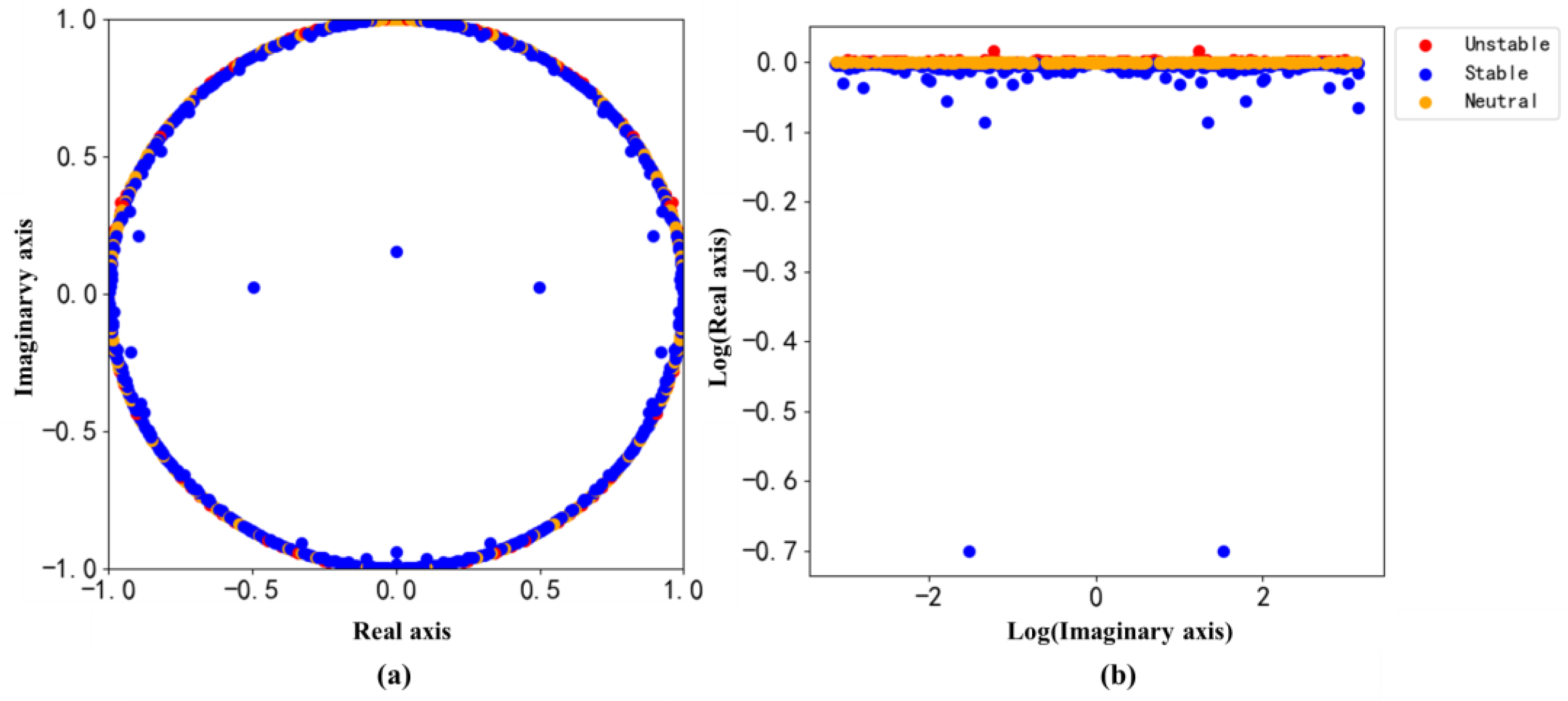
We conducted mode decomposition on hourly PM2.5 data (744 h) for the first month of 2019. In Figure 2a, the distribution of eigenvalues resulting from the modal decomposition method used is presented. Most eigenvalues are located on or near the unit circle, with only a few slightly outside of it, indicating that the decomposed modes are generally stable. In Figure 2b, the distribution of logarithmized eigenvalues is presented, where the horizontal axis represents the logarithm of the imaginary part, and the vertical axis represents the logarithm of the real part. This logarithmic view reveals that, for most modes, the logarithm of the real part is positive and close to zero, suggesting that unstable modes are gradually intensifying and dominating the dynamics of pollutant concentrations. Conversely, eigenvalues with negative real parts correspond to stabilizing modes that are diminishing over time.
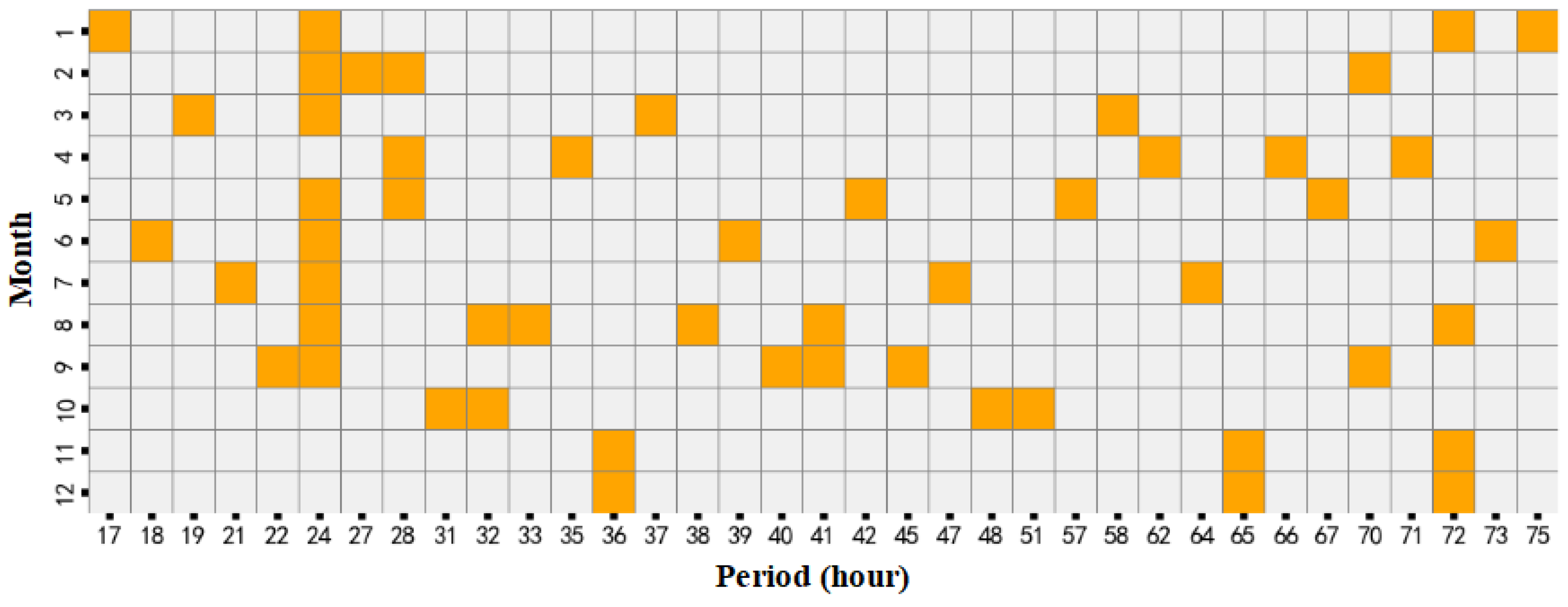
Our study decomposes the patterns of PM2.5 concentrations over the 12 months of 2019, identifying the cycles with the largest amplitude for each month, as shown in Figure 3. Throughout the year, significant patterns are observed within the 24 h and 72 h cycles, suggesting that these cycles play a dominant role in the variation in PM2.5 concentrations. Additionally, within the 24 h period, amplitude patterns have been identified at 17, 18, 21, and 22 h intervals, which likely correspond to short-term pollution events, such as brief spikes during peak traffic hours. Although these modes contribute minimally to overall concentration levels, recognizing their cyclic variations is essential for understanding the localized dynamics of PM2.5 and can aid in developing targeted and effective pollution control strategies. Furthermore, the observed 72 h cycle may be associated with weather changes or pollution accumulation processes. By identifying these key dynamic modes and frequencies, we can more accurately capture the dynamic patterns of PM2.5 concentrations and incorporate these patterns as critical features in predictive models, thereby improving the accuracy of both short- and long-term forecasts.

3.1.2. Mode Decomposition of Daily PM2.5 Concentrations

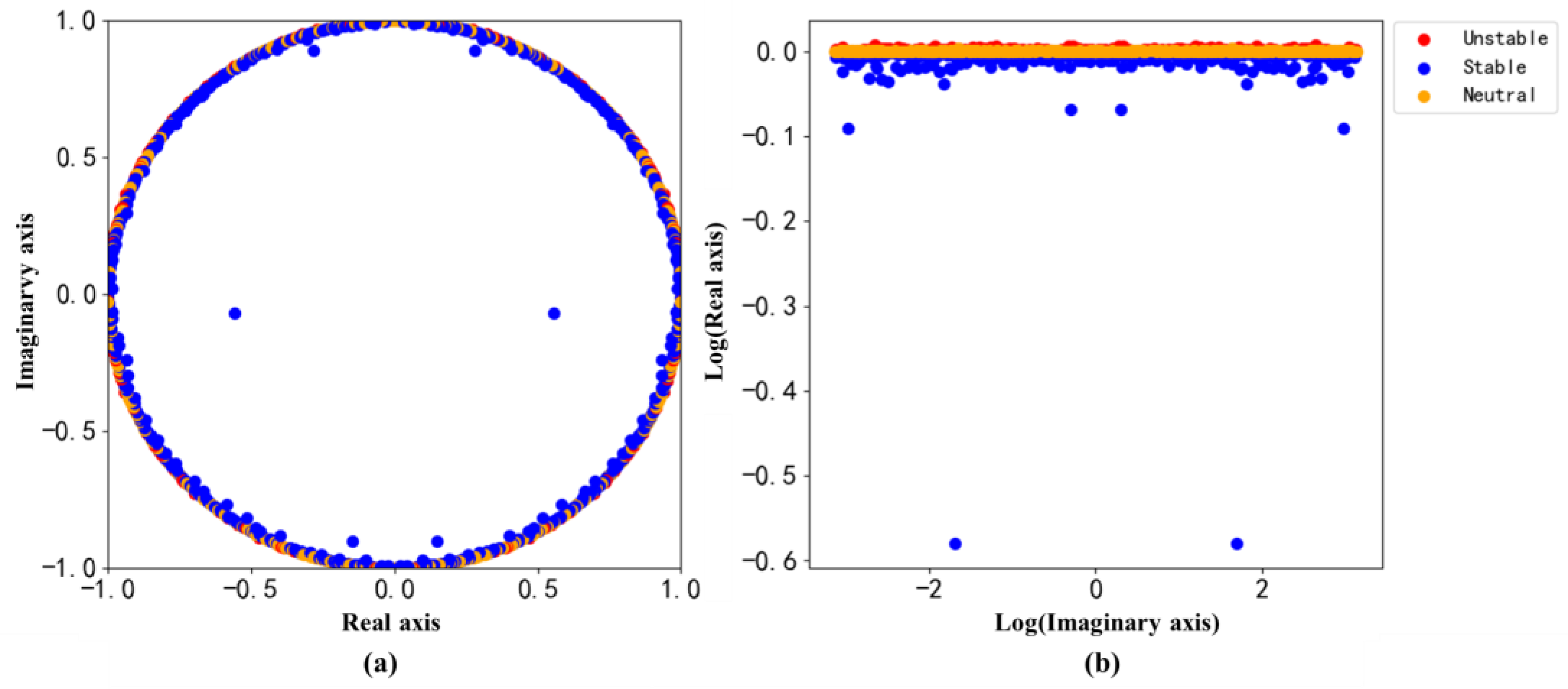
Figure 4a,b present the eigenvalue decomposition and logarithmized eigenvalues of daily PM2.5 concentrations. Figure 4a reveals that the majority of eigenvalues for the daily average PM2.5 concentrations are positioned close to the unit circle, indicating that the daily average PM2.5 exhibits predominantly stable dynamic behavior, with only a minor portion of eigenvalues suggesting instability. By contrast, Figure 4b shows that unstable patterns become progressively more pronounced over time, while stable patterns gradually diminish.
Figure 5 shows the distribution of periodicity, amplitude, and growth rate relationships for daily modal features. It is evident that the 353-day cycle has the most significant amplitude and the lowest growth rate, approaching zero at 0.00044. This indicates that this mode may represent the most prominent cycle in the evolution of PM2.5 concentrations, suggesting that the nearly annual cycle has the greatest impact on PM2.5 levels. The second most prominent cycle, with a large amplitude, is 323 days, followed by cycles of 22 days, 23 days, and 8 days. These cycles approximate annual, monthly, and weekly periods, respectively. Thus, the relationship between amplitude and period reveals that PM2.5 concentrations exhibit annual cycles (353 days and 323 days), monthly cycles (22 days and 23 days), and weekly variations (8 days). This finding aligns with the decomposition results for hourly PM2.5 concentrations, further confirming the presence of annual, monthly, weekly, and daily periodic patterns in PM2.5 levels. These periodic characteristics have also been corroborated by other related studies, reinforcing the reliability of the results [10,39].
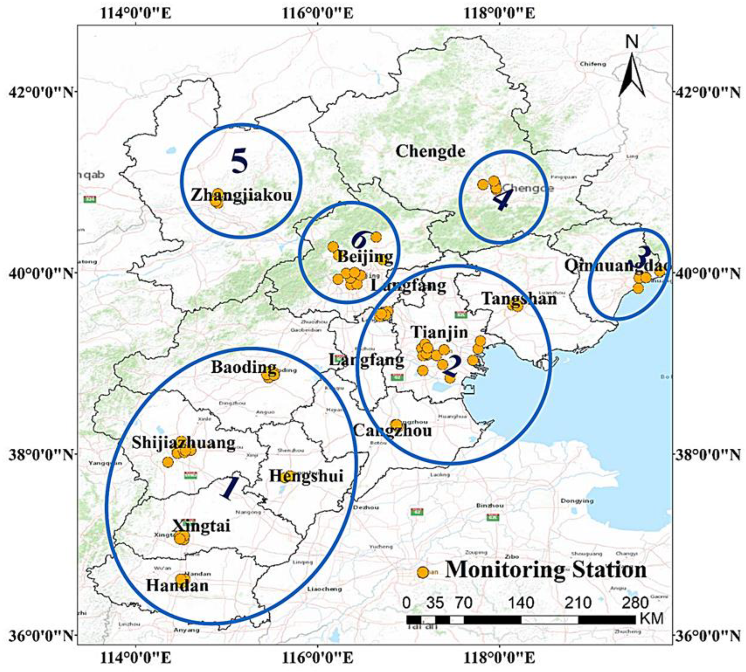
To further verify the applicability of the Koopman method for PM2.5 concentration mode decomposition at different spatial scales, the 76 monitoring stations were divided into six regions, as shown in Figure 6. This division allows for a more detailed analysis of the common characteristics and variation patterns in PM2.5 across different regions, helping to identify regional similarities and differences in pollution trends and behaviors. Regions 1, 2, and 3 are located in the southeastern part of the BTH region, which primarily encompasses industrial zones. Regions 4 and 5 are situated in the northern suburbs of the BTH, characterized by mountainous and highland terrain with fewer pollution sources. Region 6 encompasses Beijing, which represents a densely urbanized area.
To further describe the evolutionary patterns of PM2.5 pollution processes, our study defines three types of spatiotemporal dynamic modes to characterize the hierarchical structure of the pollution process. Specifically, Local Concentration Pollution (LCP) refers to oscillations that do not propagate across monitoring stations, with stations being fixed or located at certain spatial positions. Forward Concentration Pollution (FCP) indicates a continuous increase in concentration over time. Move Concentration Pollution (MCP) refers to PM2.5 pollution propagating in reverse along the monitoring stations, with the amplitude of the pollution decaying over time.
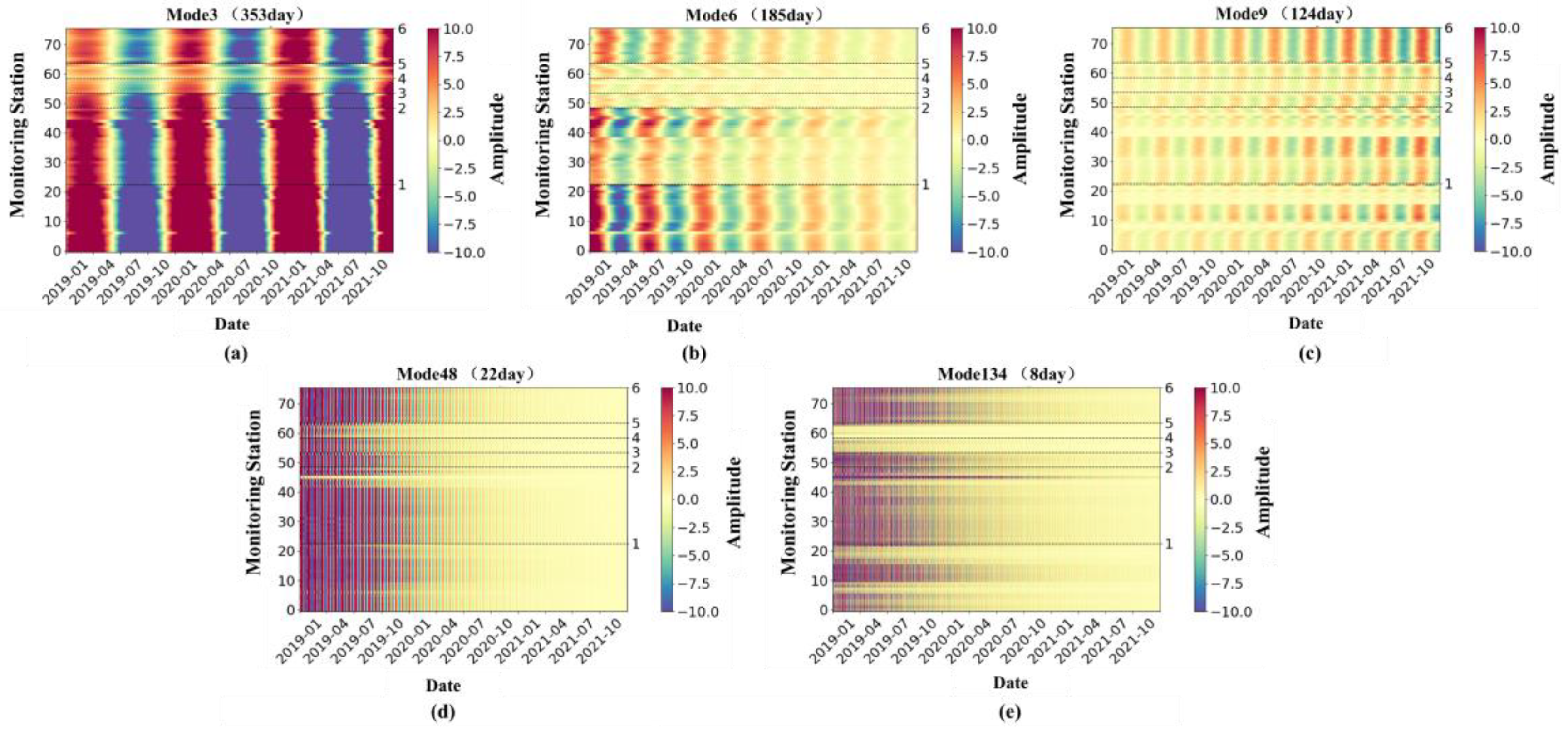
As shown in Figure 7a, Mode 3 (353 days) exhibits an annual cycle with a shared LCP structure, where its amplitude is completely confined to the front and back of the time axis. This mode decay rate is close to zero, indicating that PM2.5 contributions are highest in winter and spring each year, while pollution intensity is lower in summer and autumn. Additionally, the annual cycle displays a multi-peak structure at some monitoring stations, demonstrating the effectiveness of the Koopman method in pinpointing specific pollution sources. Modes 6 (185 days) with a semi-annual cycle, Mode 9 (124 days) with a seasonal cycle, Mode 48 (22 days) with a monthly cycle, and Mode 134 (8 days) with a weekly cycle, as shown in Figure 7b–e, all exhibit a Move Concentration Pollution (MCP) structure, indicating that the PM2.5 amplitude decays over time. This demonstrates that the KMD method can identify decaying modes, thereby reflecting changes in pollution.
Specifically, Mode 6 (185 days) with a semi-annual cycle, as shown in Figure 7b, indicates that PM2.5 concentrations were concentrated within the first 200 days of 2019, with no significant changes in pollution levels at other times. Mode 9 (124 days) with a seasonal cycle, as shown in Figure 7c, exhibits a Forward Concentration Pollution (FCP) structure, indicating that PM2.5 pollution propagates in reverse across the monitoring stations throughout the seasonal cycle. This indicates the rapid growth of PM2.5 pollution during the seasonal cycle, with the amplitude almost entirely active around the last 200 days. Mode 48 (22 days) with a monthly cycle, as shown in Figure 7d, has the highest decay rate of −0.004. Mode 134 (8 days) with a weekly cycle, as shown in Figure 7e, shows that PM2.5 concentrations gradually decrease over time, with amplitude changes mainly concentrated within the first 8 days. This reduction is speculated to be related to human activities, such as local emissions (traffic emissions), resulting in a “weekend effect.”

3.2. Reconstructing the Dynamic Process of PM2.5

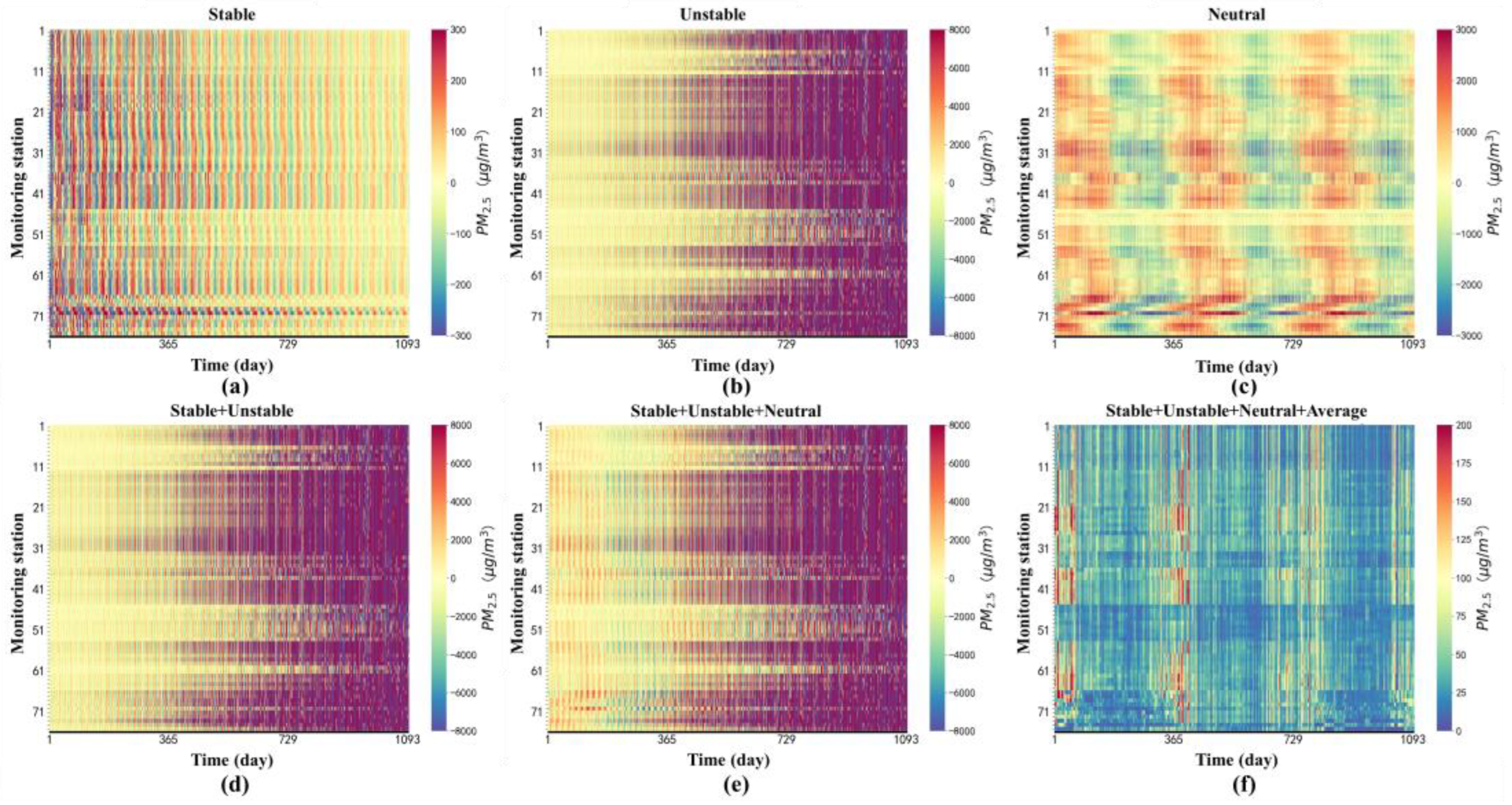
The stable, unstable, and neutral modes derived from the decomposition of PM2.5 concentrations were plotted to verify the existence of a physically meaningful connection between the modes identified in this study and the actual dynamic behavior of PM2.5. The results are presented in Figure 8a–c. Figure 8a demonstrates that the stable mode exhibits decay characteristics, Figure 8b demonstrates that the unstable mode shows growth characteristics, and Figure 8c reveals that the neutral mode displays oscillatory behavior without significant growth or decay. These modes were then superimposed, along with the previously removed mean, to reconstruct the original data, as shown in Figure 8f. The reconstruction error, measured by the MAPE, was only 0.6%. This low error rate indicates that the pattern of decomposing PM2.5 concentrations is an important sub-mode, validating the validity and accuracy of the Koopman method.
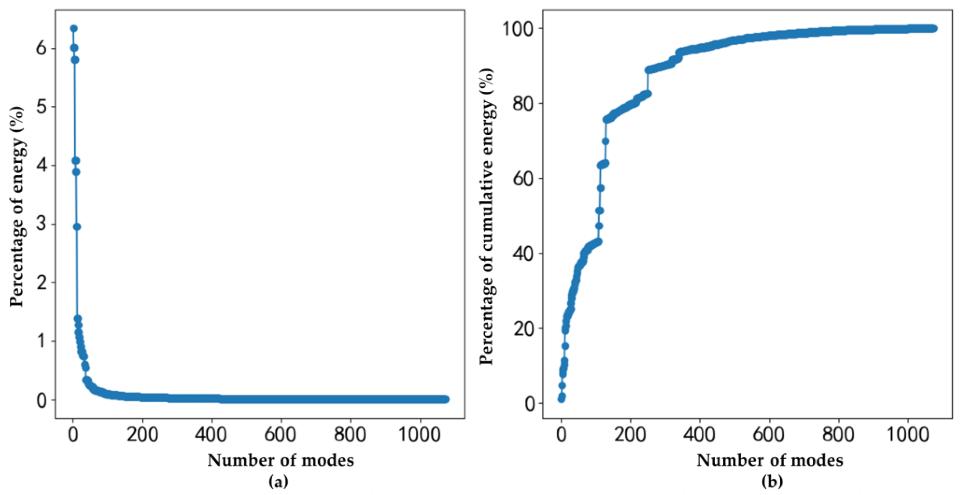
To further verify that an appropriate combination of modes can efficiently reconstruct the raw PM2.5 concentration data, this study ranks all obtained higher-order and lower-order modes by the amplitude magnitude from mode decomposition to compute the energy proportion and cumulative energy of each mode. The results are shown in Figure 8. As demonstrated in Figure 9a, the first-order modes occupy a significant proportion of the total energy, with modes of orders 2–20 accounting for 66.4% of the total energy. Figure 9b illustrates the cumulative energy percentage of the modes, showing that as the number of modes increases, the cumulative energy percentage rises and eventually stabilizes. The first 100 modes account for 42.8% of the total energy, while the first 300 modes contribute 90%, the first 400 modes contribute 95%, and the first 700 modes contribute 99% of the total energy. This indicates that the first 700 modes are the most significant in reconstructing the original data. In other words, selecting the appropriate modes can effectively achieve accurate data reconstruction.

3.3. Analysis of PM2.5 Concentration Mode Characteristics during Special Events

To validate the effectiveness of the KMD method in revealing regional pollution synchrony, the sequence of pollution occurrences, and the relationship between key pollution cities and their surrounding areas, we conducted a study on pollution events in the BTH region during a specific period. This period, spanning from 19 January 2020 to 15 February 2020, includes both the Chinese Lunar New Year and the COVID-19 lockdown.
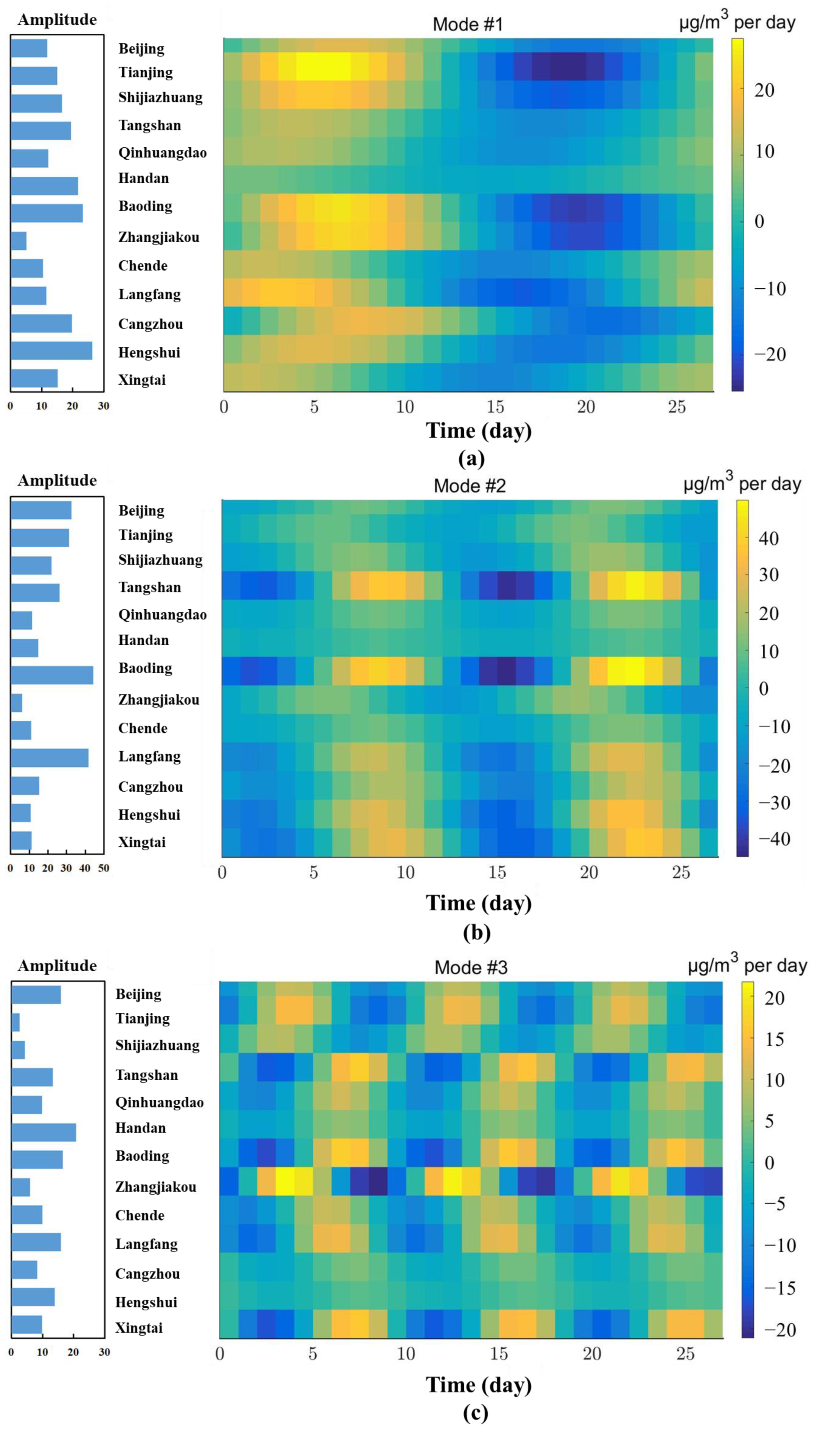
Figure 10 shows the periodicity and amplitude relationships of PM2.5 modes in 13 cities, with Figure 10b displaying the amplitudes of each mode. Mode 2 has the largest amplitude, with a period of 13.68 days. This is due to the BTH region experiencing two severe dust storm pollution events within 28 days marked by biweekly cyclic effects [40], resulting in significant amplitude fluctuations of PM2.5 concentrations during this time. Figure 10a displays the top three modes with the highest amplitudes, revealing the dynamic structure of air pollution. The periods and amplitudes of these modes reveal the severity of the pollution events, providing critical policy support for the implementation and management of regional pollution control measures.
Our study utilizes KMD method phase difference analysis to reveal the complex dynamics of PM2.5 concentration fluctuations in 13 cities of the BTH region during a brief episode of severe pollution, as shown in Figure 11. The analysis delineates Mode 1, which underscores pronounced shifts in Hengshui, Baoding, and Handan during the peak pollution phase, signaling disparate pollution levels across these locales. Modes 2 and 3 further elucidate cyclical surges of pollution in Baoding and Langfang, alongside periodic shifts in pollution levels in Handan, Baoding, Langfang, and Beijing. These findings underscore the pollution synchronicity and cyclical nature across the region. Moreover, our temporal analysis between peaks of PM2.5 concentrations reveals that smaller phase disparities align with more proximate pollution peaks.
Specifically, Mode 1 indicates that, throughout the severe pollution timeline, Langfang was afflicted by pollution three days before the subsequent batch of cities, succeeded by Beijing, Tianjin, and Shijiazhuang, with Baoding and Zhangjiakou trailing. Concurrently, Mode 2 identifies simultaneous pollution peaks in Tangshan and Baoding, while Langfang and Hengshui exhibit akin synchronous pollution events, intersecting with Xingtai. Mode 3 uncovers the finding that Tangshan, Baoding, Langfang, and Xingtai encounter uniform pollution phases, demonstrating a recurrent oscillatory pollution pattern. Contrarily, pollution in Zhangjiakou precedes other cities by three days, affirming the diverse degrees of synchronicity and sequence of pollution across the BTH region in 13 cities. This nuanced spatiotemporal examination offers crucial insights into the meticulous management of air quality and response strategies for severe pollution episodes, highlighting the imperative for crafting bespoke pollution abatement strategies.

3.4. Comparison of the Koopman Method with Other Mode Decomposition Methods

3.4.1. It Avoids Mode Mixing Compared to EMD

The EMD method is designed for handling non-stationary data series. This method decomposes signal fluctuations and trends at various scales into a series of data sequences, referred to as Intrinsic Mode Function (IMF) components [41].
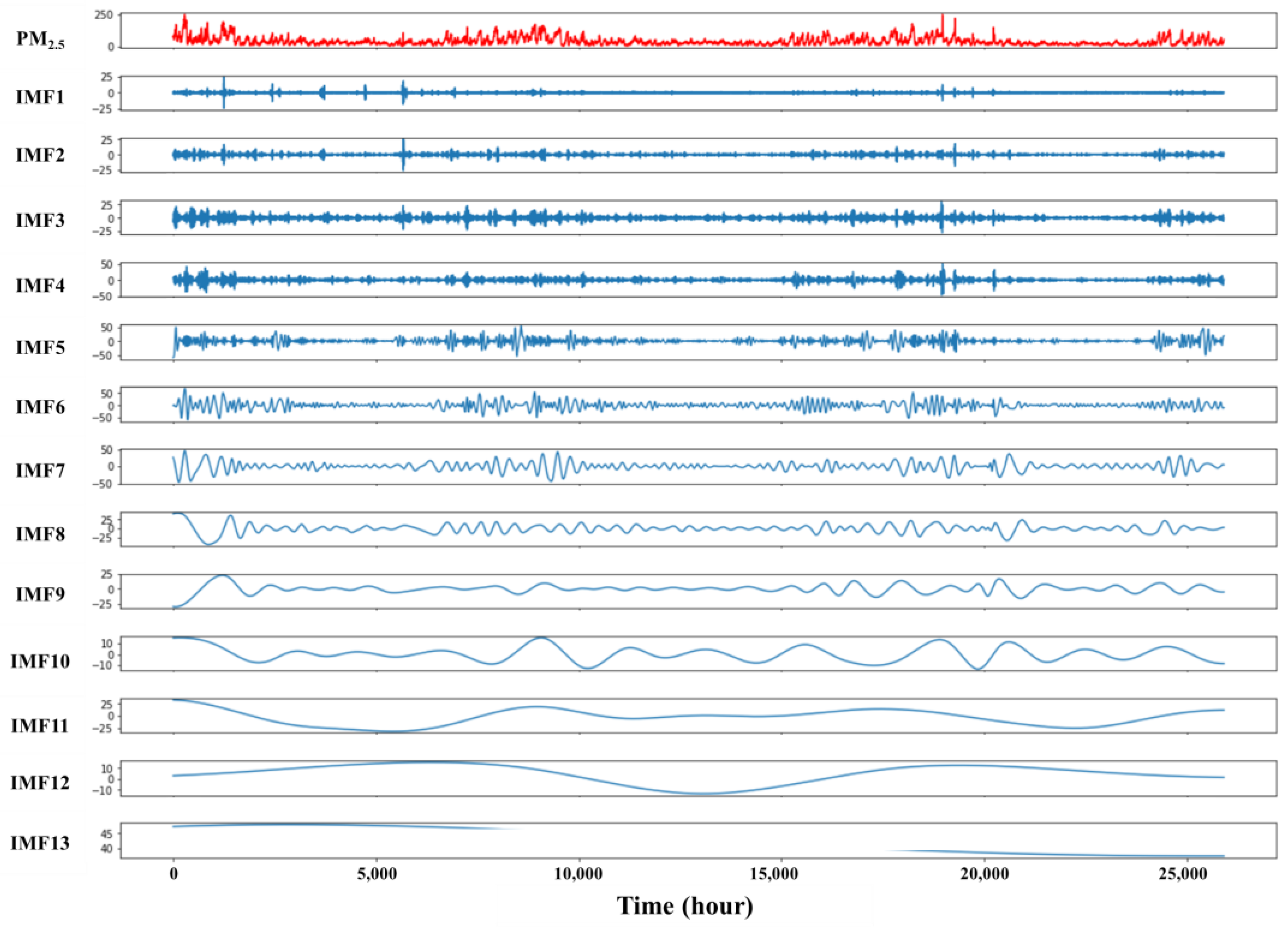
We conducted an EMD method time series decomposition of hourly PM2.5 concentrations from 2019 to 2021, as illustrated in Figure 12. The raw hourly PM2.5 concentration data exhibit fluctuations with distinct periods and peaks over the time span. The EMD method has a trend component and thirteen IMFs, each containing multiple frequency components. The high-frequency modes, IMF1 and IMF2, capture the high-frequency components of the raw signal, while the low-frequency modes, IMF12 and IMF13, capture the low-frequency components. However, the EMD method does not clearly distinguish specific oscillatory modes, indicating notable mode mixing between high-frequency and low-frequency components. By contrast, Table 1 presents the top 10 mode features obtained from the KMD method of hourly PM2.5 concentrations. Each mode in this decomposition represents distinct periods and amplitudes, effectively avoiding the mixing of information across different time scales and preventing the overlap of high-frequency and low-frequency modes. Additionally, IMF7 and IMF8 exhibit significant periodic variations and are useful for analyzing the periodic characteristics of PM2.5 concentrations. Thus, while EMD method can characterize PM2.5 concentrations at multiple scales, its mode mixing issue hampers the clear identification of individual dynamic modes, affecting the understanding and prediction of complex systems.

3.4.2. It Identifies the Key Mode Compared to Wavelet Analysis

Wavelet analysis, featuring adjustable time-frequency windows, enables localization in both the time and frequency domains [42]. This method converts time series into time-frequency representations, allowing for the identification of various patterns of variability and their temporal changes [43].
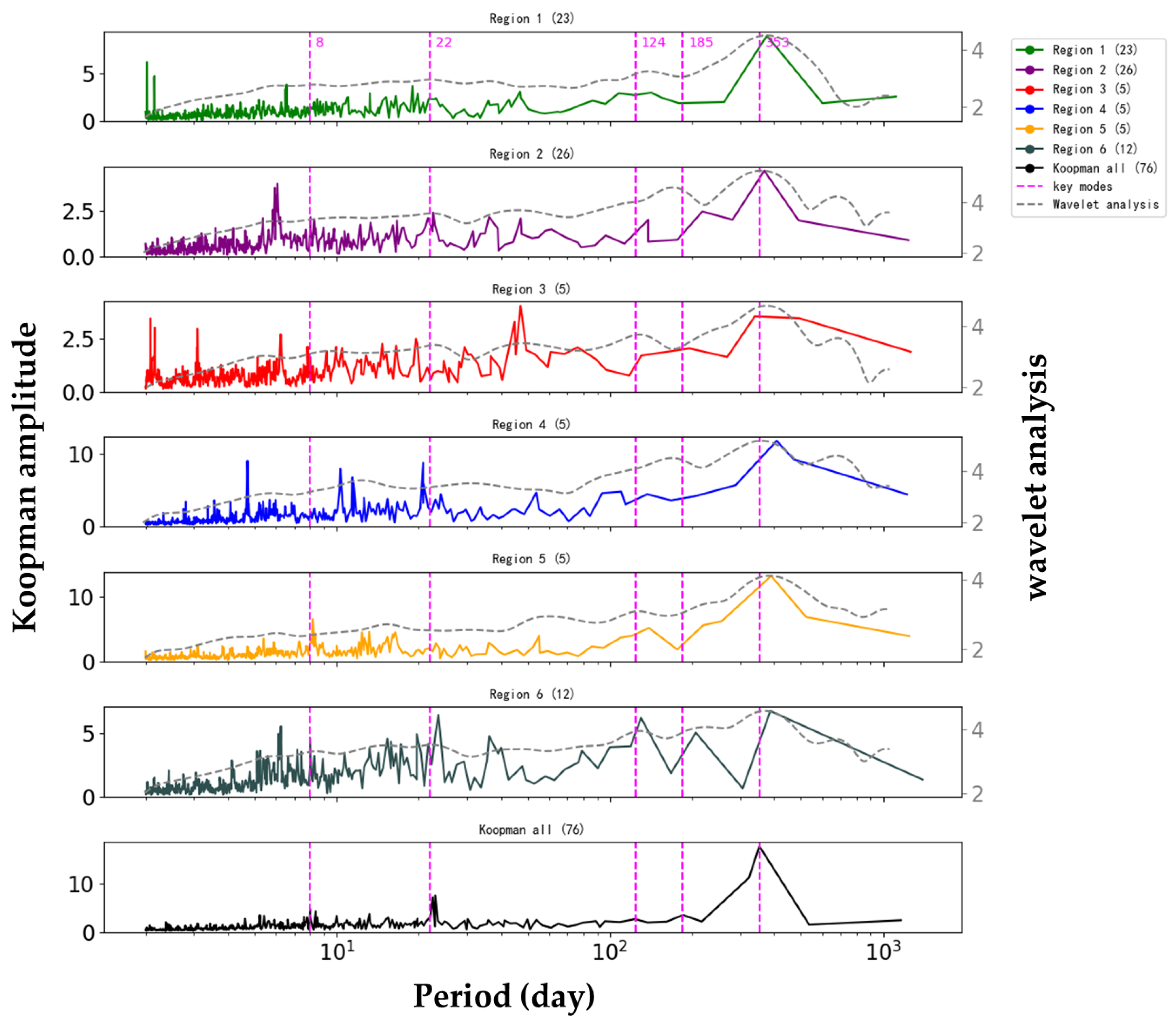
To better illustrate the differences between the KMD method and wavelet analysis, this study compares the performance of these two methods in six regions by analyzing the amplitude trends in the decomposition of PM2.5 concentration patterns, as shown in Figure 13. The KMD method performs consistently well in all regions, effectively identifying global modal features and capturing localized details, particularly in high-frequency cycles. By contrast, while wavelet analysis is effective at capturing overall trends, its output tends to be smoother, with fewer and less pronounced peaks. The discrepancy is particularly pronounced between days 13 and 20 in regions 2 and 3, where the amplitude trends diverge between the KMD method and wavelet analysis. Additionally, the KMD method’s sensitivity to high-frequency dynamic changes is evident, as it captures more amplitude peaks during the first 10 to 15 days, which may correspond to short-term pollution events. Notably, the KMD method also accurately identifies the system’s key modes, such as the dynamic modal cycles of 8, 22, 124, 185, and 353 days, as indicated by the purple dashed lines, which are consistently observed across all six regions. These observations further demonstrate the superior capability of the KMD method in accurately identifying and extracting both global and critical dynamic modes of the system.

4. Discussion

In this study, we utilized the KMD method to explore the hierarchical structure of PM2.5 concentrations across various spatial and temporal scales. This approach enabled us to identify key dynamic modes, such as growth, decay, and oscillation, and to successfully reconstruct these dynamic processes. Our analysis revealed the presence of cyclic patterns in PM2.5 concentrations on daily, weekly, monthly, seasonal, and annual scales, aligning with the findings of previous research [10,39,44]. For instance, Liu [45] observed significant spatial and diurnal variations in PM2.5 across different regions of China. In particular, the BTH region exhibited short-term cycles ranging from approximately one week to half a month, while long-term cycles were predominantly annual. Similarly, Kimothi [46] studied PM2.5 concentrations in the Himalayan region of India, noting higher concentrations and frequencies during both day and night, especially during peak tourist seasons, which were largely attributed to vehicular emissions and human activities. Mohtar [47] also reported that changes in major air pollutant concentrations in Malaysia’s urban environments were closely linked to seasonal variations, influenced by both regional and local factors. Collectively, these studies highlight the widespread occurrence of multi-scale cyclic variations in PM2.5 concentrations under different geographic and climatic conditions. By comparing our results with these studies, we further confirm the efficacy of the KMD method in uncovering the dynamic modes of PM2.5 pollution processes on a global scale.
The KMD method offers substantial advantages in analyzing complex spatiotemporal phenomena, particularly when compared to the EMD method. The EMD method often suffers from mode mixing, where high-frequency and low-frequency components overlap, complicating the separation of frequency components and potentially leading to inaccuracies in understanding and predicting PM2.5 concentrations [48,49]. By contrast, the KMD method excels at distinctly separating modes across different frequencies, ensuring the independence of each mode, thereby enhancing both the explanatory power and predictive accuracy for complex spatiotemporal processes [13]. Additionally, while wavelet analysis is frequently employed for PM2.5 concentration modal decomposition and effectively captures long-term evolutionary trends, it often fails to detect key modes that reflect local details, resulting in an incomplete interpretation of short-term dynamic changes [50,51]. Compared to these methods, the KMD method not only successfully captures global dynamic features but also identifies and resolves local dynamic modes. Therefore, when contrasted with other modal decomposition techniques [52,53], the KMD method provides a more comprehensive understanding and reconstruction of spatiotemporal processes, significantly enhancing the accuracy and reliability of predictions.
In the future, we plan to further refine the Koopman method to tackle the challenges associated with understanding and reconstructing complex spatiotemporal phenomena that involve additional variables. This will allow for a more comprehensive representation of the spatiotemporal characteristics of the data. Moreover, we intend to conduct extensive validation of the modal decomposition and prediction models to ensure their applicability and feasibility across different regions and varying conditions.

5. Conclusions

This study initially employed the KMD method to analyze the spatiotemporal hierarchical structure of hourly and daily PM2.5 concentrations, revealing hidden dynamic modes and reconstructing the dynamic processes. Subsequently, the phase difference function of the KMD method was applied to elucidate the synergistic relationships of pollution within the BTH region. Finally, the effectiveness and superiority of the KMD method were validated through a comparative analysis with the EMD method and wavelet analysis. This study’s findings are as follows:
(1)
The KMD method effectively captures the key modes of PM2.5, identifying high-frequency dominant cycles of 24 h along with low-frequency cycles on annual, semi-annual, seasonal, and monthly scales. These modes include growth, decay, and persistent sub-modes, which offer substantial interpretability and enable accurate reconstruction of the dynamic processes, with a reconstruction error MAPE of only 0.6%. Furthermore, phase difference analysis using the Koopman method elucidates the sequence, specific locations, and spatiotemporal variations in pollution across thirteen distinct cities within the BTH region.
(2)
Compared with the EMD method, the Koopman approach clearly separates each dynamic feature of PM2.5 concentration, effectively distinguishing between high-frequency and low-frequency modes, and avoiding mode mixing phenomena.
(3)
Compared with wavelet analysis, the Koopman method focuses more on the global features of the system and can accurately identify the key dynamic modes of complex systems.

Author Contributions

Conceptualization, Y.Y. and B.W.; methodology, Y.Y.; writing—original draft preparation, Y.Y.; writing—review and editing, F.Z. and D.L.; All authors have read and agreed to the published version of the manuscript.

Funding

This study was supported by the National Natural Science Foundation of China (Grant No. 42171412).

Institutional Review Board Statement

Not applicable.

Informed Consent Statement

Informed consent was obtained from all subjects involved in this study. All authors commented on the manuscript and agreed to the published version of the manuscript.

Data Availability Statement

The raw data are available at the following GitHub link: https://github.com/Koopman-123/BTH-KMD (accessed on 5 September 2024).

Acknowledgments

We kindly thank the anonymous reviewers for their helpful suggestions on a previous version of this manuscript.

Conflicts of Interest

The authors declare no conflicts of interest.

References

  1. Cohen, A.J.; Brauer, M.; Burnett, R.; Anderson, H.R.; Frostad, J.; Estep, K.; Balakrishnan, K.; Brunekreef, B.; Dandona, L.; Dandona, R. Estimates and 25-year trends of the global burden of disease attributable to ambient air pollution: An analysis of data from the Global Burden of Diseases Study 2015. Lancet 2017, 389, 1907–1918. [Google Scholar] [CrossRef]
  2. Yu, B.; Huang, C.; Liu, Z.; Wang, H.; Wang, L. A chaotic analysis on air pollution index change over past 10 years in Lanzhou, northwest China. Stoch. Environ. Res. Risk Assess. 2011, 25, 643–653. [Google Scholar] [CrossRef]
  3. Wang, F.; Chen, D.; Cheng, S.; Li, J.; Li, M.; Ren, Z. Identification of regional atmospheric PM10 transport pathways using HYSPLIT, MM5-CMAQ and synoptic pressure pattern analysis. Environ. Model. Softw. 2010, 25, 927–934. [Google Scholar] [CrossRef]
  4. Kiesewetter, G.; Schoepp, W.; Heyes, C.; Amann, M. Modelling PM2.5 impact indicators in Europe: Health effects and legal compliance. Environ. Model. Softw. 2015, 74, 201–211. [Google Scholar] [CrossRef]
  5. Lauret, P.; Heymes, F.; Aprin, L.; Johannet, A. Atmospheric dispersion modeling using artificial neural network based cellular automata. Environ. Model. Softw. 2016, 85, 56–69. [Google Scholar] [CrossRef]
  6. Sousa, S.; Martins, F.G.; Alvim-Ferraz, M.C.; Pereira, M.C. Multiple linear regression and artificial neural networks based on principal components to predict ozone concentrations. Environ. Model. Softw. 2007, 22, 97–103. [Google Scholar] [CrossRef]
  7. Qiao, W.; Tian, W.; Tian, Y.; Yang, Q.; Wang, Y.; Zhang, J. The forecasting of PM2.5 using a hybrid model based on wavelet transform and an improved deep learning algorithm. IEEE Access 2019, 7, 142814–142825. [Google Scholar] [CrossRef]
  8. Zhang, B.; Zhang, H.; Zhao, G.; Lian, J. Constructing a PM2.5 concentration prediction model by combining auto-encoder with Bi-LSTM neural networks. Environ. Model. Softw. 2020, 124, 104600. [Google Scholar] [CrossRef]
  9. Teng, M.; Li, S.; Xing, J.; Song, G.; Yang, J.; Dong, J.; Zeng, X.; Qin, Y. 24-Hour prediction of PM2.5 concentrations by combining empirical mode decomposition and bidirectional long short-term memory neural network. Sci. Total Environ. 2022, 821, 153276. [Google Scholar] [CrossRef]
  10. Guo, Y.; Quan, J.; Pan, Y.; Pu, W.; Feng, J.; Zhao, X.; Yuan, T. Multi-time scale variations of the PM2.5 in Beijing and its key mechanisms during 2008 to 2017. China Environ. Sci. 2022, 42, 1013–1021. [Google Scholar]
  11. Zaini, N.; Ean, L.W.; Ahmed, A.N.; Malek, M.A.; Chow, M.F. PM2.5 forecasting for an urban area based on deep learning and decomposition method. Sci. Rep. 2022, 12, 17565. [Google Scholar] [CrossRef]
  12. Qin, S.; Liu, F.; Wang, J.; Sun, B. Analysis and forecasting of the particulate matter (PM) concentration levels over four major cities of China using hybrid models. Atmos. Environ. 2014, 98, 665–675. [Google Scholar] [CrossRef]
  13. Avila, A.M.; Mezić, I. Data-driven analysis and forecasting of highway traffic dynamics. Nat. Commun. 2020, 11, 2090. [Google Scholar] [CrossRef]
  14. Manzoor, W.A.; Rawashdeh, S.; Mohammadi, A. Vehicular applications of koopman operator theory—A survey. IEEE Access 2023, 11, 25917–25931. [Google Scholar] [CrossRef]
  15. Kim, S.; Kim, M.; Lee, S.; Lee, Y.J. Discovering spatiotemporal patterns of COVID-19 pandemic in South Korea. Sci. Rep. 2021, 11, 24470. [Google Scholar] [CrossRef]
  16. Huynh, P.K.; Setty, A.R.; Le, T.B.; Le, T.Q. A noise-robust Koopman spectral analysis of an intermittent dynamics method for complex systems: A case study in pathophysiological processes of obstructive sleep apnea. IISE Trans. Healthc. Syst. Eng. 2023, 13, 101–116. [Google Scholar] [CrossRef]
  17. Schmid, P.J. Dynamic mode decomposition of numerical and experimental data. J. Fluid Mech. 2010, 656, 5–28. [Google Scholar] [CrossRef]
  18. Mezić, I. Analysis of fluid flows via spectral properties of the Koopman operator. Annu. Rev. Fluid Mech. 2013, 45, 357–378. [Google Scholar] [CrossRef]
  19. Bruder, D.; Gillespie, B.; Remy, C.D.; Vasudevan, R. Modeling and control of soft robots using the koopman operator and model predictive control. arXiv 2019, arXiv:1902.02827. [Google Scholar]
  20. Bruder, D.; Fu, X.; Gillespie, R.B.; Remy, C.D.; Vasudevan, R. Data-driven control of soft robots using Koopman operator theory. IEEE Trans. Robot. 2020, 37, 948–961. [Google Scholar] [CrossRef]
  21. Folkestad, C.; Pastor, D.; Burdick, J.W. Episodic Koopman learning of nonlinear robot dynamics with application to fast multirotor landing. In Proceedings of the 2020 IEEE International Conference on Robotics and Automation (ICRA), Paris, France, 31 May–31 August 2020; pp. 9216–9222. [Google Scholar]
  22. Ling, E.; Zheng, L.; Ratliff, L.J.; Coogan, S. Koopman operator applications in signalized traffic systems. IEEE Trans. Intell. Transp. Syst. 2020, 23, 3214–3225. [Google Scholar] [CrossRef]
  23. Colbrook, M.J.; Mezić, I.; Stepanenko, A. Limits and powers of Koopman learning. arXiv 2024, arXiv:2407.06312. [Google Scholar]
  24. Deng, C.; Qin, C.; Li, Z.; Li, K. Spatiotemporal variations of PM2.5 pollution and its dynamic relationships with meteorological conditions in Beijing-Tianjin-Hebei region. Chemosphere 2022, 301, 134640. [Google Scholar] [CrossRef] [PubMed]
  25. Cao, J.; Qiu, X.; Peng, L.; Gao, J.; Wang, F.; Yan, X. Impacts of the differences in PM2.5 air quality improvement on regional transport and health risk in Beijing–Tianjin–Hebei region during 2013–2017. Chemosphere 2022, 297, 134179. [Google Scholar] [CrossRef] [PubMed]
  26. Alsahli, M.M.; Al-Harbi, M. Allocating optimum sites for air quality monitoring stations using GIS suitability analysis. Urban Clim. 2018, 24, 875–886. [Google Scholar] [CrossRef]
  27. Liu, J.; He, C.; Si, Y.; Li, B.; Wu, Q.; Ni, J.; Xu, C. Toward Better and Healthier Air Quality: Global PM2.5 and O3 Pollution Status and Risk Assessment Based on the New WHO Air Quality Guidelines for 2021. Glob. Chall. 2024, 8, 2300258. [Google Scholar] [CrossRef]
  28. Cao, K.X.; Tang, M.M.; Ge, J.H.; Li, Z.K.; Wang, X.Y.; Li, G.X.; Wei, X.T. Comparison of methods to interpolate missing PM2.5 values: Based on air surveillance data of Beijing. J. Environ. Occup. Med. 2020, 37, 299–305. [Google Scholar]
  29. Ukhurebor, K.E.; Azi, S.O.; Aigbe, U.O.; Onyancha, R.B.; Emegha, J.O. Analyzing the uncertainties between reanalysis meteorological data and ground measured meteorological data. Measurement 2020, 165, 108110. [Google Scholar] [CrossRef]
  30. Koopman, B.O. Hamiltonian systems and transformation in Hilbert space. Proc. Natl. Acad. Sci. USA 1931, 17, 315–318. [Google Scholar] [CrossRef]
  31. Koopman, B.O.; Neumann, J.V. Dynamical systems of continuous spectra. Proc. Natl. Acad. Sci. USA 1932, 18, 255–263. [Google Scholar] [CrossRef]
  32. Mezić, I. Spectrum of the Koopman operator, spectral expansions in functional spaces, and state-space geometry. J. Nonlinear Sci. 2020, 30, 2091–2145. [Google Scholar] [CrossRef]
  33. Azencot, O.; Erichson, N.B.; Lin, V.; Mahoney, M. Forecasting sequential data using consistent koopman autoencoders. In Proceedings of the International Conference on Machine Learning, Vienna, Austria, 13–18 July 2020; pp. 475–485. [Google Scholar]
  34. Lusch, B.; Kutz, J.N.; Brunton, S.L. Deep learning for universal linear embeddings of nonlinear dynamics. Nat. Commun. 2018, 9, 4950. [Google Scholar] [CrossRef] [PubMed]
  35. Jovanović, M.R.; Schmid, P.J.; Nichols, J.W. Sparsity-promoting dynamic mode decomposition. Phys. Fluids 2014, 26, 024103. [Google Scholar] [CrossRef]
  36. Brunton, S.L.; Brunton, B.W.; Proctor, J.L.; Kaiser, E.; Kutz, J.N. Chaos as an intermittently forced linear system. Nat. Commun. 2017, 8, 19. [Google Scholar] [CrossRef]
  37. Takens, F. Detecting Strange Attractors in Turbulence. In Dynamical Systems and Turbulence, Warwick 1980: Proceedings of a Symposium Held at the University of Warwick 1979/80; Springer: Berlin/Heidelberg, Germany, 2006; pp. 366–381. [Google Scholar]
  38. Mezić, I.; Banaszuk, A. Comparison of systems with complex behavior. Phys. D Nonlinear Phenom. 2004, 197, 101–133. [Google Scholar] [CrossRef]
  39. Zareba, M.; Weglinska, E.; Danek, T. Air pollution seasons in urban moderate climate areas through big data analytics. Sci. Rep. 2024, 14, 3058. [Google Scholar] [CrossRef] [PubMed]
  40. Wang, Y.; Wang, H.; Zhang, S. Quantifying prediction and intervention measures for PM2.5 by a PDE model. J. Clean. Prod. 2020, 268, 122131. [Google Scholar] [CrossRef]
  41. Huang, N.E.; Wu, M.-L.C.; Long, S.R.; Shen, S.S.; Qu, W.; Gloersen, P.; Fan, K.L. A confidence limit for the empirical mode decomposition and Hilbert spectral analysis. Proc. R. Soc. Lond. Ser. A Math. Phys. Eng. Sci. 2003, 459, 2317–2345. [Google Scholar] [CrossRef]
  42. Guo, T.; Zhang, T.; Lim, E.; Lopez-Benitez, M.; Ma, F.; Yu, L. A review of wavelet analysis and its applications: Challenges and opportunities. IEEE Access 2022, 10, 58869–58903. [Google Scholar] [CrossRef]
  43. Torrence, C.; Compo, G.P. A practical guide to wavelet analysis. Bull. Am. Meteorol. Soc. 1998, 79, 61–78. [Google Scholar] [CrossRef]
  44. Shelton, S.; Liyanage, G.; Jayasekara, S.; Pushpawela, B.; Rathnayake, U.; Jayasundara, A.; Jayasooriya, L.D. Seasonal variability of air pollutants and their relationships to meteorological parameters in an urban environment. Adv. Meteorol. 2022, 2022, 5628911. [Google Scholar] [CrossRef]
  45. Liu, Z.; Ji, D.; Wang, L. PM2.5 concentration prediction based on EEMD-ALSTM. Sci. Rep. 2024, 14, 12636. [Google Scholar]
  46. Kimothi, S.; Chilkoti, S.; Rawat, V.; Thapliyal, A.; Gautam, A.S.; Gautam, S. Micro- to macro-scaling analysis of PM2.5 in sensitive environment of Himalaya, India. Geol. J. 2023, 58, 4360–4378. [Google Scholar] [CrossRef]
  47. Mohtar, A.A.A.; Latif, M.T.; Baharudin, N.H.; Ahamad, F.; Chung, J.X.; Othman, M.; Juneng, L. Variation of major air pollutants in different seasonal conditions in an urban environment in Malaysia. Geosci. Lett. 2018, 5, 21. [Google Scholar] [CrossRef]
  48. Yuan, E.; Yang, G. SA–EMD–LSTM: A novel hybrid method for long-term prediction of classroom PM2.5 concentration. Expert Syst. Appl. 2023, 230, 120670. [Google Scholar] [CrossRef]
  49. Liu, R.; Shao, M.; Wang, Q.G. Multi-timescale variation characteristics of PM2.5 in different regions of China during 2014–2022. Sci. Total Environ. 2024, 920, 171008. [Google Scholar] [CrossRef]
  50. Chen, X.; Yin, L.; Fan, Y.; Song, L.; Ji, T.; Liu, Y.; Tian, J.; Zheng, W. Temporal evolution characteristics of PM2.5 concentration based on continuous wavelet transform. Sci. Total Environ. 2020, 699, 134244. [Google Scholar] [CrossRef]
  51. Fattah, M.A.; Morshed, S.R.; Kafy, A.-A.; Rahaman, Z.A.; Rahman, M.T. Wavelet coherence analysis of PM2.5 variability in response to meteorological changes in South Asian cities. Atmos. Pollut. Res. 2023, 14, 101737. [Google Scholar] [CrossRef]
  52. Sun, W.; Li, Z. Hourly PM2.5 concentration forecasting based on mode decomposition-recombination technique and ensemble learning approach in severe haze episodes of China. J. Clean. Prod. 2020, 263, 121442. [Google Scholar] [CrossRef]
  53. Huang, G.; Li, X.; Zhang, B.; Ren, J. PM2.5 concentration forecasting at surface monitoring sites using GRU neural network based on empirical mode decomposition. Sci. Total Environ. 2021, 768, 144516. [Google Scholar] [CrossRef]
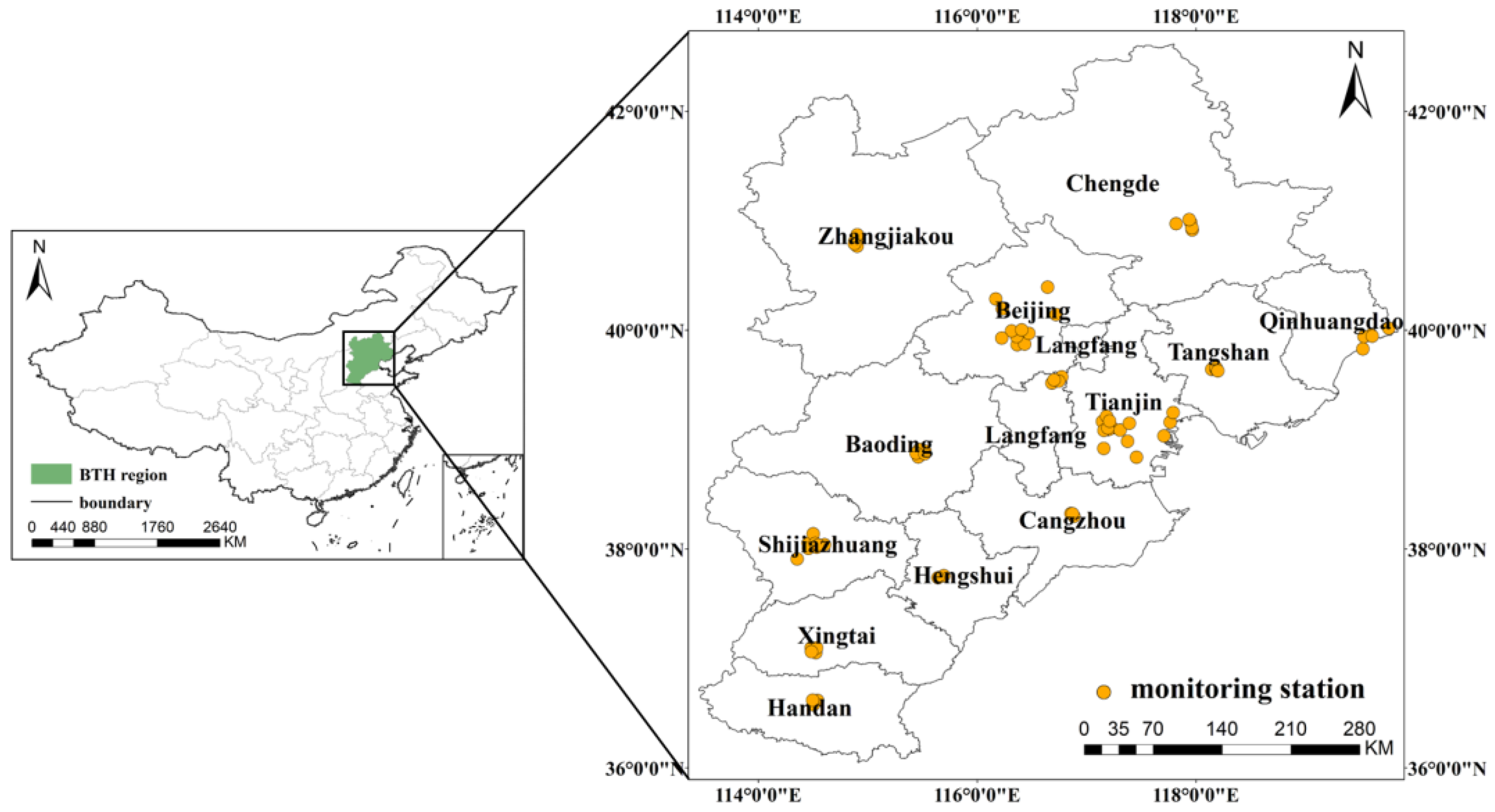
Figure 1. Map of China and location of the BTH region.
Atmosphere 15 01091 g001
Figure 2. (a) Plotting the eigenvalues of hourly PM2.5 concentrations on the unit circle reveals that Koopman eigenvalues are symmetrically distributed as conjugate pairs within the unit circle. (b) The logarithmized amplitudes of these hourly PM2.5 concentration modes are displayed, highlighting their decay rates. The decay rate is taken as the negative of the real part of the eigenvalue.
Atmosphere 15 01091 g002
Figure 3. Periodic distributions corresponding to the larger amplitudes obtained from the decomposition of hourly PM2.5 concentrations over the 12 months of 2019.
Atmosphere 15 01091 g003
Figure 4. (a) Eigenvalues of PM2.5 daily concentration patterns plotted on the unit circle. (b) Logarithmized distribution of eigenvalues of daily PM2.5 concentrations.
Atmosphere 15 01091 g004
Figure 5. Distribution of amplitude, period, and growth rate for daily PM2.5: (a) amplitude vs. period for PM2.5. The red circle highlights several periodic points (353 days, 323 days, 23 days and 22 days). At these specific cycle lengths, the PM2.5 concentration changes exhibit significant regularity, indicating a strong periodic influence on pollution levels. (b) amplitude and growth rate distribution of PM2.5, with the positive eigenvalue real part indicating growth rate.
Atmosphere 15 01091 g005
Figure 6. Zoning of 76 sites in the BTH region: 23 stations in region 1 (Baoding, Shijiazhuang, Hengshui, Xingtai, Handan), 26 stations in region 2 (Langfang, Tianjin, Tangshan, Cangzhou), 5 stations in region 3 (Qinhuangdao), 5 stations in region 4 (Chengde), 5 stations in region 5 (Zhangjiakou), and 12 stations in region 6 (Zhangjiakou).
Atmosphere 15 01091 g006
Figure 7. Koopman modes for major cycle variations are as follows: (a) the mode distribution structure of the annual cycle; (b,d,e) share the same mode structure, manifesting as decaying modes; (c) represents the growing mode structure of the seasonal cycle.
Atmosphere 15 01091 g007
Figure 8. Koopman mode analysis of daily PM2.5: (ac) stable, unstable, and neutral modes; (d,e) various modes superimposed on each other; (f) reconstruction of PM2.5 concentration modes through the superposition of stable, unstable, neutral, and average.
Atmosphere 15 01091 g008
Figure 9. Percentage of energy and percentage of cumulative energy for PM2.5 mode amplitudes. (a) Percentage of energy of amplitude, and (b) percentage of cumulative energy of amplitude.
Atmosphere 15 01091 g009
Figure 10. (a) Decomposition of 28-day characteristic values in heavy pollution, with the top three modes with the highest amplitude being represented by # 1, # 2, and # 3; (b) amplitudes of each pattern.
Atmosphere 15 01091 g010
Figure 11. Heavy pollution average phase and amplitude of the first three modes in the BTH region. (a) Average phase and amplitude distribution for Mode 1; (b) average phase and amplitude distribution for Mode 2; (c) average phase and amplitude distribution for Mode 3.
Atmosphere 15 01091 g011
Figure 12. The EMD method was applied to hourly PM2.5, distinguishing 13 modes.
Atmosphere 15 01091 g012
Figure 13. Comparison of wavelet analysis and the KMD method at different spatial scales. The left y-axis shows the amplitude of the KMD method for calculating the daily average PM2.5 concentrations for the six regions, while the right y-axis shows the amplitude from the wavelet analysis. The purple dashed lines represent the key dynamic mode periods (8, 22, 124, 185, and 353 days) identified by the KMD method. The numbers in parentheses indicate that the six regions contain 23, 26, 5, 5, 5, and 12 monitoring stations, respectively. The Koopman method was applied to all stations within each region, whereas wavelet analysis was conducted using a single representative station from each region. Furthermore, the Koopman method was also utilized for the modal decomposition of the 76 monitoring stations across the BTH region.
Atmosphere 15 01091 g013
Table 1. Periods and amplitudes of the top 10 modes for hourly PM2.5.
ModePeriod (Hourly)Amplitude
1735.6719.503
6123.3518.457
4178.3218.355
2364.8215.459
3248.4613.915
3123.88813.469
5156.729.942
1171.2689.3099
3024.3138.5047
1452.6818.4439
Disclaimer/Publisher’s Note: The statements, opinions and data contained in all publications are solely those of the individual author(s) and contributor(s) and not of MDPI and/or the editor(s). MDPI and/or the editor(s) disclaim responsibility for any injury to people or property resulting from any ideas, methods, instructions or products referred to in the content.