Wildfire CO₂ Emissions in the Conterminous United States from 2015 to 2018 as Estimated by the WRF-Chem Assimilation System from OCO-2 XCO₂ Retrievals

Abstract

Wildfires are becoming more frequent due to the global climate change. Large amounts of greenhouse gases emitted by wildfires can lead to increases in extreme climate events. Accurately estimating the greenhouse gas carbon dioxide (CO₂) emissions from wildfires is important for mitigation of climate change. In this paper, we develop a novel method to estimate wildfire CO₂ emissions from the relationship between local CO₂ emissions and XCO₂ anomalies. Our method uses the WRF-Chem assimilation system from OCO-2 XCO₂ retrievals which coupled with Data Assimilation Research Testbed (DART). To validate our results, we conducted three experiments evaluating the wildfire CO₂ emissions over the conterminous United States. The four-month average wildfire emissions from July to October in 2015∼2018 were estimated at 4.408 Tg C, 1.784 Tg C, 1.514 Tg C and 2.873 Tg C, respectively. Compared to the average of established inventories CT2019B, FINNv1.5 and GFASv1.2 fire emissions, our estimates fall within one standard deviation, except for 2017 due to lacking of OCO-2 XCO₂ retrievals. These results suggest that the regional carbon assimilation system, such as WRF-Chem/DART, using OCO-2 XCO₂ retrievals has a great potential for accurately tracking regional wildfire emissions.

1. Introduction

Wildfires occurring either naturally or ignited by humans are an important component of the global carbon cycle. It emits a variety of greenhouse, reactive gases and aerosols to the atmosphere, including carbon dioxide (CO₂), carbon monoxide (CO), oxides of nitrogen (NO_x), methane (CH₄), volatile and semivolatile organic compounds (VOC and SVOC), particulate matter (PM), ammonia (NH₃), sulfur dioxide (SO₂) and so on. This not only cause the immediate release of carbon stored in vegetation into the atmosphere, but also induce a long-term shift in the balance between the carbon sequestration by plants and carbon liberation through decomposition of dead biomass. This will affect the atmospheric composition and thermal balance in both the global and regional scales [1,2,3,4,5,6]. In recent decades, varying degrees of wildfires happened now and then in Australia, California, Siberia and Indonesia. These wildfires had a significant impact on the ecological environment, human health, and economic life in these regions [7,8,9,10]. Wang et al. [11] use a combination of physical, epidemiological and economic models to estimate the economic impacts of California wildfires in 2018. The estimation result shows that the wildfire damages in 2018 totaled $148.5 (126.1–192.9) billion (roughly 1.5% of California’s annual gross domestic product).

Wildfires affect climate through direct carbon dioxide CO₂ emissions and multiple postfire carbon source and sink pathways. Globally, since 2000, CO₂ emissions from fossil fuels and land-use change averaged 9 billion metric tons of carbon (Gt C) per year, whereas wildfire CO₂ emissions were approximately 2 Gt C per year [12]. Over the past few decades, the increasing frequency of wildfires is a concerning trend that is linked to the global warming [13]. In the conterminous United States, the increase in burned area from wildfires has roughly quadrupled. This trend is concerning because wildfires can contribute to the accumulation of greenhouse gases in the atmosphere, which in turn leads to further global warming. Many studies have analyzed various aspects of the atmospheric impacts of wildfires, ranging from the more general such as air quality issue and emissions assessment, to more specific or local including particulate matter emissions, transport, radiative effects and so on [14]. Miranda et al. [15] estimated CO₂ emissions due to wildfires and found that in years when the burnt area exceeds 100,000 ha, this contribution could reach 7% of the total Portuguese CO₂ emissions. So, it is important to study the variation of wildfire CO₂ emissions on both global and regional scales which will improve our understanding of the damage from wildfires. The analysis of wildfires CO₂ emissions can provide a valuable foundation for decision-makers to formulate relevant policies.

The variety of satellites and observation data provide conveniences for the estimation of the wildfire CO₂ emissions scale and the real-time monitoring of fire points [16,17,18,19]. Different research groups produced the wildfire CO₂ emissions dataset such as Global Fire Emission Database (GFED) [20,21], Fire INventory from NCAR (FINN) [22], Global Fire Assimilation System (GFAS) [23] by using the burning area (BA) and fire radiative power (FRP). Where the FRP observed by satellite data such as Moderate Resolution Imaging Spectroradiometer (MODIS). Konovalov et al. [24] propose a method to estimate the wildfires CO₂ emissions in Siberia. This method use Infrared Atmospheric Sounding Interferometer (IASI) carbon monoxide (CO) retrievals and MODIS Aerosol Optical Depth (AOD) combined with outputs from the CHIMERE mesoscale chemistry-transport model. The study found the “top-down” estimates for the total annual biomass burning CO₂ emissions in the period from 2007 to 2011 in Siberia are by factors of 2.5 and 1.8 larger than the respective bottom-up estimates, such as GFED3.1 and GFASv1.0 global emission inventories. Heymann et al. [25] estimate the Indonesian fire CO₂ emissions by using the column-averaged dry air mole fraction of CO₂ (${\mathrm{XCO}}_2$) which derived from measurements of the Orbiting Carbon Observatory-2 (OCO-2) satellite mission. The estimated wildfire CO₂ emissions is 748 ± 209 Mt CO₂, which is about 30% lower than GFEDv4s and GFASv1.2. Guo et al. [26,27] successively evaluated the CO₂ emissions from the 2010 fires in western Russia by using Greenhouse Gases Observing Satellite (GOSAT) data, from the 2015 fires in Siberia by using OCO-2 data. Wang et al. [28] studies the 2019–2020 Australian mega-bushfires based on OCO-2 ${\mathrm{XCO}}_2$ retrievals. Find the smoke from wildfires can greatly obscure satellite observations, making the available ${\mathrm{XCO}}_2$ mainly locate over outer fringes of plumes downwind of the major mega-bushfires in eastern Australia in three orbit observations during November-December 2019 with their enhancements of approximately 1.5 ppm. By using an atmospheric transport model, the fire-induced CO₂ enhancement is further confirmed. The simulation experiment also suggests that the sensitivity of the downwind maximum ${\mathrm{XCO}}_2$ enhancement is 0.41 ± 0.04 ppm for 1 Tg C d⁻¹ fire emissions.

In this paper, we assess the wildfire CO₂ emissions in conterminous United States from July to October in 2015∼2018 with the regional CO₂ assimilation inversion system [29]. It can improve the regional CO₂ concentrations by assimilating OCO-2 ${\mathrm{XCO}}_2$ retrievals with WRF-Chem coupled with extending the DART [30]. We evaluate our results with CT2019B, FINNv1.5 and GFASv1.2 wildfire emissions databases.

The paper is organized as follows, the detail description of the estimate method and materials are presented in the Section 2; Results of the experiments and discussion are given in Section 3, followed by the conclusion in Section 4.

2. Materials and Methods

2.1. A Regional CO₂ Transport Model

WRF-Chem model version 4.4 was used as regional CO₂ transport model. The study area is the conterminous United States, the time range is from July to October in 2015∼2018. The physics and chemistry configurations of WRF-ChemV4.4 is showed in

Table 1. Physics and chemistry configurations of the WRF-Chem V4.4.

Options	Configurations
WRF_Core	ARW
Domain center	${34.939}^{\circ }$ N–${96.275}^{\circ }$ W
Grid resolution	50 km
nx,ny,nz	103,82,45
Interval seconds	21,600 s/6 h
Time steps	240 s
Start date	2015~01-07-2018 00:00:00
End date	2015~01-11-2018 00:00:00
Microphysics process	WSM 5-class simple ice scheme [31]
Cumulus parameterization	Kain-Fritsch scheme [32]
Longwave atmospheric radiation	RRTM scheme [33]
Shortwave atmospheric radiation	Dudhia scheme [34]
Planetary boundary layer scheme	MYNN 2.5 level TKE [35]
Surface layer scheme	MYNN [36]
Land surface scheme	Unified Noah Land surface model
Chemistry option	chem_opt = 16 (CO2 only)

[29].

The WRF-Chem model use ds083.2 data (https://rda.ucar.edu/datasets/ds083.2/, accessed on 15 November 2023) as the initial meteorological dataset, which is $1^{\circ }\times 1^{\circ }$ spatial resolution and 6-hourly temporal resolution from National Centers for Environmental Prediction (NCEP) FNL Operational Model Global Tropospheric Analyses, continuing from July 1999.

The initial and boundary conditions of CO₂ concentrations on WRF-Chem model are interpolated from CT2019B CO₂ total mole fractions products which is $3^{\circ }\times 2^{\circ }$ spatial resolution and three-hourly temporal resolution. The prior CO₂ flux is CT2019B flux which is $1^{\circ }\times 1^{\circ }$ spatial resolution and three-hourly temporal resolution, including anthropogenic emissions, fire emissions, biogenic fluxes, and ocean fluxes.

2.2. CO₂ Concentration Assimilation System

The study is based on the regional CO₂ concentration assimilation system with OCO-2 ${\mathrm{XCO}}_2$ retrievals by extending DART [29,30].

The ${\mathrm{XCO}}_2$ retrievals from nadir observation mode with good quality according to the “xco2_quality_flag” are selected from the OCO-2 Level2 (L2) Lite data product V10 and its preprocessing method is as below [29]:

$$\widetilde{OCO{2}_{XC{O}_2}}=\sum _{i=1}^{n}OCO{2}_{XC{O}_{2i}}{\sigma }_{OCO{2}_i}^{-2}/\sum _{i=1}^n{\sigma }_{OCO{2}_i}^{-2}$$

(1)

$$\widetilde{{\sigma }_{OCO2}}=1/\sqrt{N^{-1}\sum _{i=1}^n{\sigma }_{OCO{2}_i}^{-2}}$$

(2)

where $\widetilde{OCO{2}_{XC{O}_2}}$ and $\widetilde{{\sigma }_{OCO2}}$ denotes the representative mean ${\mathrm{XCO}}_2$ value and its uncertainty of a model grid cell respectively.

According to the strategy of Crowell et al. [37], the observation operator H was implemented to link the OCO-2 10 s mean ${\mathrm{XCO}}_2$ retrievals to the CO₂ concentration forecast by WRF-Chem model, which is defined as:

$$XC{O}_2^m=XC{O}_2^a+\sum _j{h}_j{a}_j(C{O}_2^m-C{O}_2^a)$$

(3)

where $XC{O}_2^a$, $h_j$, $a_j$ and $C{O}_2^a$ are the prior ${\mathrm{XCO}}_2$ value, the pressure weighting function, the column averaging kernel and the prior CO₂ concentration profile used by OCO-2 ${\mathrm{XCO}}_2$ retrieval process respectively. $C{O}_2^m$ is the optimal CO₂ concentration profile which interpolated to the pressure levels of OCO-2 ${\mathrm{XCO}}_2$ retrieval from WRF-Chem model. $XC{O}_2^m$ is the column-average CO₂ concentration of the WRF-Chem forecasts which converted by the operator H.

The assimilation system used Ensemble Adjustment Kalman Filter (EAKF) [38] as the data assimilation approach, and advanced by WRF-Chem to next assimilation cycle. Let $x_k^{init}$, $x_k^f$, $x_k^a$ represent the initial states of the prior CO₂ concentration distribution, the forecast states advanced by WRF-Chem starting from $x_k^{init}$ and the analysis states of the k-th ensemble member of each assimilation cycle, respectively. The $x_k^{init}$ was generated in the same way as that of Mizzi et al. [39] by imposing a Gaussian distribution around mean values of CO₂ concentrations calculated from CT2019B as the initial background with a 5% standard deviation about the mean. The forecast states $x_k^f$ were transformed into the observation space by the observation operator H, i.e., $y_{m,k}^f$ = $H\left(x_k^f\right)$, where the subscript m means “from model”. The analysis result of each $y_{m,k}^f$ was calculated as:

$$y_{m,k}^a=\left[\sqrt{\frac{{\widetilde{{\sigma }_{OCO2}}}^2}{{\widetilde{{\sigma }_{OCO2}}}^2+{\overline{\sigma }}_m^{f^2}}}\right]\left[y_{m,k}^f-{\overline{y}}_m^f\right]+\left[\frac{{\overline{y}}_m^f}{{\overline{\sigma }}_m^{f^2}}+\frac{{\widetilde{OCO2}}_{XC{O}_2}}{{\widetilde{{\sigma }_{OCO2}}}^2}\right]{\left[\frac{1}{{\overline{\sigma }}_m^{f^2}}+\frac{1}{{\widetilde{{\sigma }_{OCO2}}}^2}\right]}^{-1}$$

(4)

where ${\widetilde{OCO2}}_{XC{O}_2}$ is the representative mean ${\mathrm{XCO}}_2$ values of a model grid cell with uncertainty $\widetilde{{\sigma }_{OCO2}}$ calculated from the OCO-2 retrievals by Equations (1) and (2). ${\overline{y}}_m^f$ is the ensemble forecast mean with ensemble spread ${\overline{\sigma }}_m^{f^2}$ in the observation space. At the end of each assimilation cycle, the analysis state of the k-th ensemble member was updated as:

$$x_k^a=x_k^f+\alpha \frac{\sigma (x^f,y_m^f)}{{\overline{\sigma }}_m^{f^2}}(y_{m,k}^a-y_{m,k}^f)$$

(5)

where $\sigma (x^f,y_m^f)$ is the covariance of $x^f$ and $y_m^f$ across the ensemble. $\alpha$ is a covariance localization function to compensate the sampling error due to small ensemble size [40].

2.3. Wildfire Emissions Estimate Model

Hakkarainen et al. [41,42] indicates a positive correlation between ${\mathrm{XCO}}_2$ anomalies and CO₂ emission inventories in regional-scale, which can be defined as:

$$\Delta F=\lambda \ast \Delta XC{O}_2$$

(6)

where $\Delta F$ is CO₂ emissions, $\Delta XC{O}_2$ is the ${\mathrm{XCO}}_2$ anomalies corresponding to CO₂ emissions, $\lambda$ is the positive correlation coefficient.

We propose a model to estimate the wildfire CO₂ emissions in the conterminous United States. First we design two simulation experiments to compute the positive correlation coefficient $\lambda$. The difference between two simulation experiments is whether to add the wildfire emissions to the prior flux or not. Where the $\Delta XC{O}_2$ is the ${\mathrm{XCO}}_2$ anomalies derived from the two simulation experiments results. $\Delta F$ is the wildfire CO₂ emissions. Then we design one CO₂ assimilation experiment to estimate the wildfire emissions in conterminous United States with the known coefficient $\lambda$ and ${\mathrm{XCO}}_2$ anomalies. So, we obtain an equation about CO₂ emissions increment and ${\mathrm{XCO}}_2$ increment in the wildfire area, which defined as follows:

$$\frac{\Delta Flux1}{\Delta XCO2\_1}=\frac{\Delta Flux2}{\Delta XCO2\_2}$$

(7)

where $\Delta Flux1$ and $\Delta Flux2$ represent two CO₂ flux increment respectively, the $\Delta XCO2\_1$ and $\Delta XCO2\_2$ are the ${\mathrm{XCO}}_2$ increment corresponding to the above two CO₂ flux increment.

2.4. Wildfire Emissions of CT2019B

By analyzing the CT2019B monthly total CO₂ fluxes, anthropogenic CO₂ emissions, biological CO₂ fluxes, fire CO₂ emissions and ocean CO₂ fluxes from 2000 to 2018 in conterminous United States, we found the monthly mean anthropogenic CO₂ emissions does not change significantly with time, while the monthly mean biogenic CO₂ fluxes has obvious seasonal and inter-annual changes.

In the total CO₂ fluxes, the proportion of wildfire CO₂ emissions is less than 7%. Large-scale wildfires typically occurred in summer, particularly in August and September, and this trend has been increasing year by year from 2000 to 2018. As Figure 1 shows, in the year 2015∼2018, the wildfires occurred in July and August of each year mainly at northwest area of the conterminous United States, and the wildfire in August is larger than July. While in September and October the wildfire also appeared at southeast area of the conterminous United States.

2.5. Experiment Design

In this paper, we design three groups of comparative experiments. Two $C{O}_2$ concentration simulation experiments named as “SIM_EXP1” and “SIM_EXP2”, one $C{O}_2$ concentration assimilate experiment with the OCO-2 $XC{O}_2$ retrievals named as “DA_EXP3”. The configurations of the three experiments are shown in

Table 2. The configurations of the three experiments.

Experiment Name	Initial and Boundary	Prior Flux	Assimilate or Not	Experiment Time
SIM_EXP1	CT2019B CO2 total mole fractions products	CT2019B optimized fluxes with fire emissions	NO	July to October of 2015∼2018
SIM_EXP2	CT2019B CO2 total mole fractions products	CT2019B optimized fluxes without fire emissions	NO	July to October of 2015∼2018
DA_EXP3	CT2019B CO2 total mole fractions products	CT2019B optimized fluxes without fire emissions	YES	July to October of 2015∼2018

.

The two simulation experiments SIM_EXP1, SIM_EXP2 were designed to demonstrate the significant impact of wildfire emissions on ${\mathrm{XCO}}_2$. For SIM_EXP1, the initial and boundary conditions of the WRF-Chem were interpolated from CT2019B CO₂ total mole fractions products, the prior CO₂ flux was interpolated from CT2019B total fluxes which include anthropogenic emissions, fire emissions, biogenic fluxes, and ocean fluxes. For SIM_EXP2, the initial and boundary conditions were the same as SIM_EXP1, but the prior CO₂ fluxes only include anthropogenic emissions, biogenic fluxes and ocean fluxes.

For DA_EXP3 experiment, we optimizing the CO₂ concentrations further by assimilating with OCO-2 ${\mathrm{XCO}}_2$ retrievals [30,38,43]. The prior fluxes are same as SIM_EXP2. The initial and boundary conditions was interpolated from CT2019B CO₂ total mole fractions products, and then adding a Gaussian perturbation which the average value is 0, standard deviation is 2% to each grid point of each ensemble. In this CO₂ assimilation experiment, the size of ensemble members is set to 20, adopting Three-dimensional Gaspari-Cohn localization function [44] to compensate for sampling errors caused by the finite ensemble number. Where the influence radius in the horizontal of Three-dimensional Gaspari-Cohn localization function is 0.1 radians. In vertical, the principle of localization function is same as Kang et al. [45], which has a larger impact coefficient in lower troposphere (the sigma level of OCO-2 is 0.947) and descending to both sides. Simultaneously, we discard the observations that is 3 times larger than the prior value by implementing the exception value detection.

2.6. Wildfire Emissions Estimate Method

According to the three experiments results, the Equation (7) can be rewrite as:

$$\frac{\Delta F_{exp1-exp2}}{X_{exp1}-X_{exp2}}=\frac{\Delta F_{wildfire}}{X_{exp3}-X_{exp2}}$$

(8)

where the $X_{exp1}$, $X_{exp2}$ and $X_{exp3}$ are the mean ${\mathrm{XCO}}_2$ of SIM_EXP1, SIM_EXP2 and DA_EXP3. $\Delta F_{exp1-exp2}$ represents the CT2019B wildfire CO₂ emissions between SIM_EXP1 and SIM_EXP2, $\Delta F_{wildfire}$ is the estimated wildfire emissions in conterminous United States from our study.

To estimate the wildfire emissions accurately, we add the monthly ratio of wildfire emissions with OCO-2 ${\mathrm{XCO}}_2$ retrievals days as a variable. Let i represent one month, $D_{wildfire}^i$ represent the days of wildfire occurs in one month, $D_{total}^i$ represent total days of one month. Then the monthly ratio ${\rho }^i$ defined as:

$$\begin{array}{c}\hfill {\rho }^i=\frac{D_{wildfire}^i}{D_{total}^i}\end{array}$$

(9)

The estimated wildfire CO₂ emissions $\Delta F_{wildfire}^i$ can be computed as:

$$\begin{array}{cc}\hfill & \Delta XCO2\_1^i=X_{exp1}^i-X_{exp2}^i\hfill \end{array}$$

(10)

$$\begin{array}{cc}\hfill & \Delta XCO2\_2^i=X_{exp3}^i-X_{exp2}^i\hfill \end{array}$$

(11)

$$\begin{array}{cc}\hfill & \Delta F_{wildfire}^i=\Delta F_{exp1-exp2}^i\times \frac{\Delta XCO2\_2^i}{\Delta XCO2\_1^i}\times {\rho }^i\hfill \end{array}$$

(12)

2.7. Evaluation Data

Three different types of wildfire CO₂ emissions were used to evaluate the wildfire CO₂ emissions in conterminous United States which estimated by our method. Including CT2019B fire emissions, CAMS GFASv1.2 wildfire CO₂ emissions datasets (https://ads.atmosphere.copernicus.eu/cdsapp#!/dataset/cams-global-fire-emissions-gfas?tab=overview, accessed on 15 November 2023) [46,47] with ${0.1}^{\circ }\times {0.1}^{\circ }$ spatial resolution and FINNv1.5 fire emissions (https://www.acom.ucar.edu/Data/fire/, accessed on 15 November 2023) [22].

In our study, we also consider the influence of OCO-2 ${\mathrm{XCO}}_2$ retrievals in wildfire areas. Before evaluating the wildfire CO₂ emissions based on the Equations (10)–(12), it is necessary to select the days with sufficient OCO-2 ${\mathrm{XCO}}_2$ retrievals in wildfire areas.

Table 3. The OCO-2 ${\mathrm{XCO}}_2$ observations days in wildfire areas of the conterminous United States from July to October of 2015∼2018.

Year	July	August	September	October
2015	9	8	8	6
2016	6	7	10	10
2017	12	0	3	6
2018	10	14	18	18

shows the selected days in conterminous United States from July to October of 2015∼2018. As there are no OCO-2 ${\mathrm{XCO}}_2$ retrievals in August 2017, the number of days that can be selected is zero.

The CT2019B CO₂ concentrations and NCEP Reanalysis2 Gaussian Grid 10 m wind data were used to analysis the variation of wildfire CO₂ emissions in the conterminous United States.

2.8. Evaluation Metrics

Our experiments results were evaluated by Standard Deviation (STDE), defined as:

$$\begin{array}{c}\hfill STDE=\sqrt{\frac{{\sum }_{i=1}^n{(f_i-\overline{f})}^2}{n-1}}\end{array}$$

(13)

where n is the 3, means the three kinds of wildfire emissions as mentioned in Section 2.7. $f_i$ represent one of the three types of wildfire emissions. $\overline{f}$ is the averaged wildfire emissions of CT2019B, GFASv1.2, FINNv1.5.

3. Results and Discussion

3.1. ${\mathit{XCO}}_2$ Experiments Results

Table 4. The monthly average ${\mathrm{XCO}}_2$ of SIM_EXP1, SIM_EXP2, DA_EXP3 and CT2019B from July to October of 2015∼2018 in conterminous United States.

Year	Month	SIM_EXP1 (ppm)	SIM_EXP2 (ppm)	DA_EXP3 (ppm)	CT2019B (ppm)
2015	July	398.60	398.58	398.22	398.29
	August	397.13	397.09	396.59	396.65
	September	397.67	397.65	397.61	397.36
	October	399.19	399.18	398.98	398.81
2016	July	402.06	402.06	401.41	401.86
	August	401.13	401.12	400.49	400.51
	September	401.22	401.21	401.12	400.77
	October	402.45	402.45	402.46	402.07
2017	July	404.77	404.76	403.69	404.21
	August	402.49	402.47	401.52	402.05
	September	402.97	402.95	403.01	402.45
	October	404.43	404.43	404.41	404.01
2018	July	405.83	405.82	405.39	405.61
	August	405.12	405.07	404.67	404.80
	September	405.68	405.66	405.56	405.21
	October	406.74	406.73	406.75	406.28

shows the monthly average ${\mathrm{XCO}}_2$ of SIM_EXP1, SIM_EXP2, DA_EXP3 and CT2019B from July to October of 2015∼2018 in conterminous United States, with the CT2019B ${\mathrm{XCO}}_2$ added as reference. As the Table 4 shows, the average annual increase in ${\mathrm{XCO}}_2$ is approximately 2.57 ppm for the three experiments. The monthly averaged ${\mathrm{XCO}}_2$ exhibits an uptrend from August to October every year, especially in October, where ${\mathrm{XCO}}_2$ increases by 1.47 ppm, 1.27 ppm, 1.45 ppm, 1.11 ppm from 2015 to 2018 respectively.

Due to the absence of wildfire emissions in the prior fluxes of WRF-ChemV4.4 model, the monthly averaged ${\mathrm{XCO}}_2$ of SIM_EXP2 is 0.02 ppm lower than SIM_EXP1 in conterminous United States. The monthly averaged ${\mathrm{XCO}}_2$ of DA_EXP3 is closer to CT2019B than SIM_EXP1 and SIM_EXP2, indicating the assimilation of OCO-2 ${\mathrm{XCO}}_2$ retrievals can optimize the ${\mathrm{XCO}}_2$ distribution and make it more consistent with the CarbonTracker products.

3.2. Wildfire CO₂ Emissions Experiments Results

Due to satellite transit time, clouds and aerosols, OCO-2 satellite only has several days in which it can detect wildfire in conterminous United States from July to October. To accurately estimate monthly wildfire CO₂ emissions, the days we selected are those with OCO-2 ${\mathrm{XCO}}_2$ retrievals coupled with wildfires.

Figure 2 shows the spatial distribution of monthly mean CT2019B wildfire CO₂ emissions with 10 m wind speed and wind direction in upper panel, the monthly mean $\Delta XC{O}_2$ between DA_EXP3 and SIM_EXP2 with sufficient OCO-2 ${\mathrm{XCO}}_2$ retrievals days in lower panel, the time range is from July to October in 2015∼2018.

As the Figure 2 shows, compared with SIM_EXP2, after assimilating with OCO-2 ${\mathrm{XCO}}_2$ retrievals, the ${\mathrm{XCO}}_2$ increment of DA_EXP3 mainly locate in or around the wildfire areas. Taking into account the distribution and numeric value of the OCO-2 ${\mathrm{XCO}}_2$ retrievals, the range of wildfire occurrences in the conterminous United States, the 10 m wind speed and wind direction in different months and the CO₂ assimilate system, the ${\mathrm{XCO}}_2$ increment is primarily located in the north and east, and SIM_EXP2 having a larger ${\mathrm{XCO}}_2$ than DA_EXP3 in the other regions in July and August. In September and October, the ${\mathrm{XCO}}_2$ increment mainly locate in northwest and southeast regions where the wildfire occurs, and the negative value of $\Delta XC{O}_2$ is less than July and August.

Figure 3 shows the comparison between mean wildfire CO₂ emissions of CT2019B, FINNv1.5, GFASv1.2 and estimates in our study. The monthly mean wildfire emissions of CT2019B, FINNv1.5, GFASv1.2 and our study are presented in

Table 5. The wildfire CO₂ emissions of CT2019B, FINNv1.5, GFASv1.2 and our study in the conterminous United States from July to October in 2015∼2018.

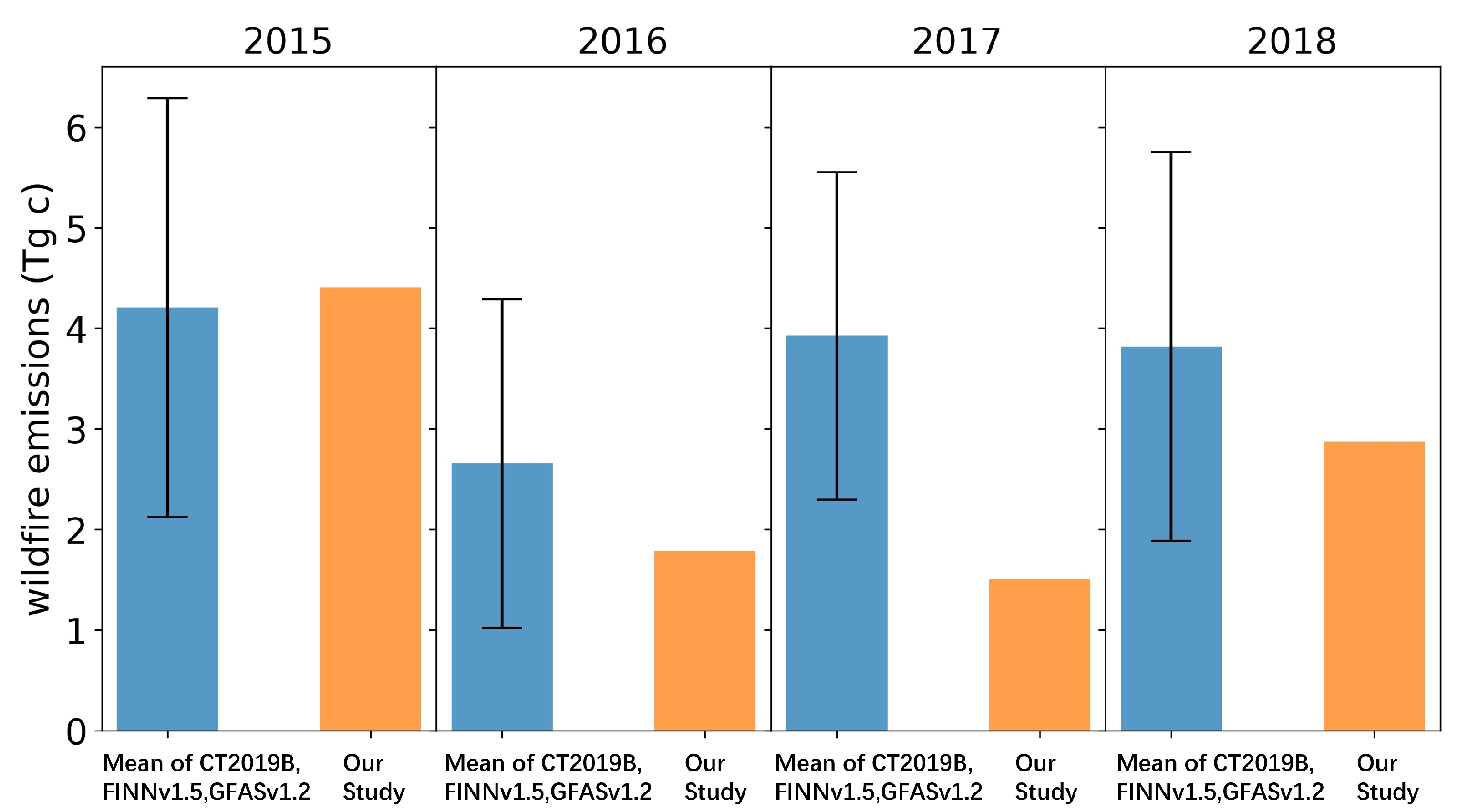
Year	Wildfire Emissions(Tg C)	July	August	September	October	Mean
2015	CT2019B	0.537	8.614	3.356	1.450	3.489
	FINNv1.5	1.840	7.238	1.872	2.246	3.299
	GFASv1.2	1.154	18.391	1.319	2.481	5.836
	Mean of CT2019B, FINNv1.5,GFASv1.2	1.177 ± 0.652	11.414 ± 6.081	2.182 ± 1.053	2.059 ± 0.541	4.208 ± 2.082
	Our study	3.568	8.251	1.552	4.263	4.408
2016	CT2019B	0.875	1.729	1.765	0.954	1.331
	FINNv1.5	1.827	2.506	2.725	3.475	2.633
	GFASv1.2	4.341	6.714	3.269	1.693	4.004
	Mean of CT2019B, FINNv1.5,GFASv1.2	2.348 ± 1.791	3.650 ± 2.682	2.586 ± 0.761	2.041 ± 1.296	2.656 ± 1.633
	Our study	0.511	0.791	3.999	1.834	1.784
2017	CT2019B	1.202	4.204	4.622	1.210	2.810
	FINNv1.5	1.553	4.664	6.629	3.949	4.199
	GFASv1.2	6.803	3.317	6.982	1.966	4.767
	Mean of CT2019B, FINNv1.5,GFASv1.2	3.186 ± 3.137	4.062 ± 0.685	6.078 ± 1.273	2.375 ± 1.415	3.925 ± 1.627
	Our study	1.758	NA	0.733	2.052	1.514
2018	CT2019B	1.556	3.568	1.620	0.733	1.869
	FINNv1.5	3.905	7.771	2.918	3.168	4.441
	GFASv1.2	6.071	8.340	4.803	1.354	5.142
	Mean of CT2019B, FINNv1.5,GFASv1.2	3.844 ± 2.258	6.560 ± 2.607	3.114 ± 1.600	1.752 ± 1.265	3.817 ± 1.933
	Our study	2.087	3.061	4.100	2.246	2.873

. In our study, the four-month mean wildfire emissions in 2015 are 4.408 Tg C (1 Tg C = ${10}^{12}$ g C), which is 26.34% higher than CT2019B, 33.63% higher than FINNv1.5 and 24.47% lower than GFASv1.2. These values fall within one standard deviation of the average values of CT2019B, FINNv1.5 and GFASv1.2 (4.208 ± 2.082 Tg C).

The four-month mean wildfire emissions in 2016 is 1.784 Tg C, is 34.05% larger than CT2019B, 32.26% lower than FINNv1.5 and 55.45% lower than GFASv1.2. While in 2017, because of the lack of OCO-2 observation data in August and September, the evaluation of wildfire emissions with our study is inaccurate, the four-month mean wildfire emissions of our study have a large gap with the other three emissions databases. And the four-month mean wildfire emissions in 2018 is 2.873 Tg C, is 53.72% larger than CT2019B, 35.29% lower than FINNv1.5 and 44.12% lower than GFASv1.2, which also falls within one standard deviation of the average of other three wildfire emissions.

The differences in wildfire CO₂ emissions between different data sources are significant for each month. For instance, in August 2015, the wildfire CO₂ emissions of GFASv1.2 are 18.391 Tg C, where those of FINNv1.5 are 7.238 Tg C. In October 2015, the wildfire CO₂ emissions in our study are 4.263 Tg C, higher than all the others. The similar phenomenon also occurred in 2016∼2018, and the gap may be caused by the different estimation methods, model errors, different CO₂ satellites observation data and so on. For example, GFAS use the top-down approach to calculate the biomass burning emissions by assimilating FRP observations from the MODIS instruments onboard the Terra and Aqua satellites. It corrects the gaps in the observations, considers the omission errors due to the undetected small fires, using atmospheric reactive gas simulations to produce the real time daily, ${0.5}^{\circ }\times {0.5}^{\circ }$ grid, global wildfire emissions. But the occurrence of a plume may be wrongly predicted or not predicted at all in situations with extreme variability in the fire activity. FINN use the bottom-up approach to provide daily, 1 km resolution, global estimates of emissions from open fires based on the Terra and Aqua from MODIS instruments satellite detection of hot spots. This method mainly uses the fire hot spots to estimate the wildfire emissions, ignoring the impact of smaller fires on CO₂ emissions. And the use of assumed area burned, land cover maps, biomass consumption estimates, and emission factors all will introduce error into the model estimates. This leads to highly underestimation of the fire emissions in global, then causing the uncertainties and the large fluctuations in regional. CarbonTracker provides 3-hourly, $1^{\circ }\times 1^{\circ }$ grid, global estimates of surface-atmosphere CO₂ fluxes. For fire emissions, it uses GFED as one of the fire modules to estimate biomass burning. The burned area is based on MODIS satellite observations of fire counts, together with detailed vegetation cover information and a set of vegetation specific scaling factors. Based on the burned area estimate, the seasonally changing vegetation and soil biomass stocks in the CASA model are combusted and converted to atmospheric trace gases using estimates of fuel loads, combustion completeness, and burning efficiency. The diversity of wildfire CO₂ emissions estimation methods will induce the difference in estimation results, but it also promotes the progress of the estimation methods.

3.3. Effect of OCO-2 ${\mathit{XCO}}_2$ Retrievals

For each subgraph of Figure 4, the left panel shows the spatial distribution of CT2019B wildfire emissions with 10 m wind speed and wind direction, and the 10 s averaged OCO-2 ${\mathrm{XCO}}_2$ retrievals with nadir mode, the right panel shows the latitude variation of 10 s average OCO-2 ${\mathrm{XCO}}_2$ retrievals with nadir mode.

As the Figure 4a shows, the massive wildfire occurs in the northwest area of the conterminous United States, accompanied by north winds near the OCO-2 observation area. Taking the observations of the northernmost in the wildfire area as the background value, the maximum increment of OCO-2 ${\mathrm{XCO}}_2$ retrievals is about 5.17 ppm. In Figure 4b, a larger wildfire occurs in northwest region, but that day has south winds. Using observations from southernmost in the wildfire area as the background value, the maximum increment of OCO-2 ${\mathrm{XCO}}_2$ retrievals is approximately 3.16 ppm. In Figure 4c, the wildfire occurs in northwest and southeast region, but the OCO-2 observations mainly located in the center by southeast accompanied by north wind, the OCO-2 observations have an obvious upward trend in the southeast where the wildfire area, the maximum increment of OCO-2 ${\mathrm{XCO}}_2$ retrievals is about 3.92 ppm. In Figure 4d, the wildfire mainly occurs in southeast region, accompanied by southwest wind, the maximum increment of OCO-2 ${\mathrm{XCO}}_2$ retrievals is about 1.91 ppm.

Then analysis the ${\mathrm{XCO}}_2$ of DA_EXP3 with the same select days are shown in Figure 4. The daily average ${\mathrm{XCO}}_2$ distribution of SIM_EXP1, SIM_EXP2, DA_EXP3 and $\Delta XC{O}_2$ between them are shown in Figure 5. In Figure 5a, the average ${\mathrm{XCO}}_2$ of SIM_EXP1, SIM_EXP2 and DA_EXP3 in the northwest area of conterminous United States are 398.193 ppm, 398.192 ppm, 398.673 ppm respectively. Comparing with SIM_EXP1 and SIM_EXP2, the ${\mathrm{XCO}}_2$ increment of DA_EXP3 mainly locate in northwest region where wildfire occurs and northeast region where no wildfire. As Figure 4a shows the wildfire areas, the distribution of OCO-2 ${\mathrm{XCO}}_2$ retrievals and the wind direction, The ${\mathrm{XCO}}_2$ increment of northeast region may affect by the north wind in northwest region and west wind in southwest region.

In Figure 5b, the ${\mathrm{XCO}}_2$ of SIM_EXP2 is smaller than SIM_EXP1 due to the lack of wildfire CO₂ emissions in the northwest of conterminous United States. After assimilating OCO-2 ${\mathrm{XCO}}_2$ retrievals, the ${\mathrm{XCO}}_2$ of DA_EXP3 has shown improvement in regions affected by wildfires. Compared to SIM_EXP2, the results are more aligned with those of SIM_EXP1. This suggests that assimilating OCO-2 ${\mathrm{XCO}}_2$ retrievals are effective in correcting deviations in CO₂ concentration that are caused by wildfire emissions. Besides, the ${\mathrm{XCO}}_2$ distribution of DA_EXP3-SIM_EXP2 and DA_EXP3-SIM_EXP1 in other area of conterminous United States mainly due to the change of the initial CO₂ concentration in each assimilation cycle.

In Figure 5c, the difference of ${\mathrm{XCO}}_2$ between SIM_EXP1 and SIM_EXP2 is small in the southeast of conterminous United States. After assimilation, the ${\mathrm{XCO}}_2$ of DA_EXP3 in the east region increased by assimilate with OCO-2 ${\mathrm{XCO}}_2$ retrievals, wind speed and wind direction (Figure 4c). However, the ${\mathrm{XCO}}_2$ of DA_EXP3 in the middle region decreased due to the smaller OCO-2 ${\mathrm{XCO}}_2$ retrievals in this area, and this phenomenon indicates that the wildfire CO₂ emissions in SIM_EXP1 may be underestimated.

In Figure 5d, the difference of ${\mathrm{XCO}}_2$ between SIM_EXP1 and SIM_EXP2 is mainly in the southeast of conterminous United States where the wildfire occurs. Compared with the ${\mathrm{XCO}}_2$ of DA_EXP3, the results of SIM_EXP1 and SIM_EXP2 are smaller in southwest and middle north region, but larger in southeast, this may be affected by atmospheric transmission, wind speed, wind direction and prior fluxes.

From 2016 to 2018, The selected spatial distribution of CT2019B wildfire CO₂ emissions, OCO-2 ${\mathrm{XCO}}_2$ retrievals with nadir mode, the 10 m wind speed and wind direction shows in Appendix A.

4. Conclusions

In this paper, we evaluate the wildfire CO₂ emissions in conterminous United States estimated by the regional CO₂ assimilation system with OCO-2 ${\mathrm{XCO}}_2$ retrievals. The results is shown that the four-month (July to October) averaged wildfire CO₂ emissions in 2015-2018 are 4.408 Tg C, 1.784 Tg C, 1.514 Tg C, 2.873 Tg C respectively. The results are fall within one standard deviation of the estimates from CT2019B, FINNv1.5 and GFASv1.2, except for 2017, even though the wildfire CO₂ emissions has a big gap between different datasets in monthly. And the reason that the estimates of CO₂ emissions in 2017 has larger uncertainty is the lack of OCO-2 ${\mathrm{XCO}}_2$ retrievals in August and September 2017.

The results indicate the potential of the regional carbon assimilation inversion system for estimating regional wildfire CO₂ emissions. However, due to the representiveness error of the observations, model error of the chemical transport model and assimilation algorithm, the results of this study still have uncertainty. It needs more works to improve the method for quantifying the wildfires CO₂ emissions more accurately.

References

- Andreae, M.O.; Merlet, P. Emission of trace gases and aerosols from biomass burning. Glob. Biogeochem. 2001, 15, 955–966. [Google Scholar] [CrossRef]
- Change, I.C. Contribution of working groups I, II and III to the fourth assessment report of the intergovernmental panel on climate change. Synth. Rep. 2007. [Google Scholar]
- Langmann, B.; Duncan, B.; Textor, C.; Trentmann, J.; van der Werf, G.R. Vegetation fire emissions and their impact on air pollution and climate. Atmos. Environ. 2009, 43, 107–116. [Google Scholar] [CrossRef]
- Jaffe, D.A.; Wigder, N.L. Ozone production from wildfires: A critical review. Atmos. Environ. 2012, 51, 1–10. [Google Scholar] [CrossRef]
- Bond, T.C.; Doherty, S.J.; Fahey, D.W.; Forster, P.M.; Berntsen, T.; DeAngelo, B.J.; Flanner, M.G.; Ghan, S.; Kärcher, B.; Koch, D.; et al. Bounding the role of black carbon in the climate system: A scientific assessment. J. Geophys. Res. Atmos. 2013, 118, 5380–5552. [Google Scholar] [CrossRef]
- Lorenz, K.; Lal, R. Introduction. In Carbon Sequestration in Forest Ecosystems; Springer: Dordrecht, The Netherlands, 2010; pp. 1–21. [Google Scholar]
- Mead, M.I.; Castruccio, S.; Latif, M.T.; Nadzir, M.S.M.; Dominick, D.; Thota, A.; Crippa, P. Impact of the 2015 wildfires on Malaysian air quality and exposure: A comparative study of observed and modeled data. Environ. Res. Lett. 2018, 13, 044023. [Google Scholar] [CrossRef]
- Burke, M.; Driscoll, A.; Heft-Neal, S.; Xue, J.; Burney, J.; Wara, M. The changing risk and burden of wildfire in the United States. Proc. Natl. Acad. Sci. USA 2021, 118, e2011048118. [Google Scholar] [CrossRef]
- Li, A.X.; Wang, Y.; Yung, Y.L. Inducing Factors and Impacts of the October 2017 California Wildfires. Earth Space Sci. 2019, 6, 1480–1488. [Google Scholar] [CrossRef]
- Rooney, B.; Wang, Y.; Jiang, J.H.; Zhao, B.; Zeng, Z.C.; Seinfeld, J.H. Air quality impact of the Northern California Camp Fire of November 2018. Atmos. Chem. Phys. 2020, 20, 14597–14616. [Google Scholar] [CrossRef]
- Wang, D.; Guan, D.; Zhu, S.; Kinnon, M.M.; Geng, G.; Zhang, Q.; Zheng, H.; Lei, T.; Shao, S.; Gong, P.; et al. Economic footprint of California wildfires in 2018. Nat. Sustain. 2021, 4, 252–260. [Google Scholar] [CrossRef]
- Zheng, B.; Ciais, P.; Chevallier, F.; Yang, H.; Canadell, J.G.; Chen, Y.; van der Velde, I.R.; Aben, I.; Chuvieco, E.; Davis, S.J.; et al. Record-high CO2 emissions from boreal fires in 2021. Science 2023, 379, 912–917. [Google Scholar] [CrossRef]
- Bond-Lamberty, B.; Peckham, S.D.; Ahl, D.E.; Gower, S.T. Fire as the dominant driver of central Canadian boreal forest carbon balance. Nature 2007, 450, 89–92. [Google Scholar] [CrossRef] [PubMed]
- Rosa, I.M.D.; Pereira, J.M.C.; Tarantola, S. Atmospheric emissions from vegetation fires in Portugal (1990–2008): Estimates, uncertainty analysis, and sensitivity analysis. Atmos. Chem. Phys. 2011, 11, 2625–2640. [Google Scholar] [CrossRef]
- Miranda, A.; Coutinho, M.; Borrego, C. Forest fire emissions in Portugal: A contribution to global warming? Environ. Pollut. 1994, 83, 121–123. [Google Scholar] [CrossRef]
- Shi, Y.; Yamaguchi, Y. A high-resolution and multi-year emissions inventory for biomass burning in Southeast Asia during 2001–2010. Atmos. Environ. 2014, 98, 8–16. [Google Scholar] [CrossRef]
- Ross, A.N.; Wooster, M.J.; Boesch, H.; Parker, R. First satellite measurements of carbon dioxide and methane emission ratios in wildfire plumes. Geophys. Res. Lett. 2013, 40, 4098–4102. [Google Scholar] [CrossRef]
- Ban, Y.; Zhang, P.; Nascetti, A.; Bevington, A.R.; Wulder, M.A. Near Real-Time Wildfire Progression Monitoring with Sentinel-1 SAR Time Series and Deep Learning. Sci. Rep. 2020, 10, 1322. [Google Scholar] [CrossRef] [PubMed]
- Liu, X.; He, B.; Quan, X.; Yebra, M.; Qiu, S.; Yin, C.; Liao, Z.; Zhang, H. Near Real-Time Extracting Wildfire Spread Rate from Himawari-8 Satellite Data. Remote Sens. 2018, 10, 1654. [Google Scholar] [CrossRef]
- Van Der Werf, G.R.; Randerson, J.T.; Giglio, L.; Van Leeuwen, T.T.; Chen, Y.; Rogers, B.M.; Mu, M.; Van Marle, M.J.E.; Morton, D.C.; Collatz, G.J.; et al. Global fire emissions estimates during 1997–2016. Earth Syst. Sci. Data 2017, 9, 697–720. [Google Scholar] [CrossRef]
- Van der Werf, G.R.; Randerson, J.T.; Giglio, L.; Collatz, G.J.; Mu, M.; Kasibhatla, P.S.; Morton, D.C.; DeFries, R.S.; Jin, Y.; Van Leeuwen, T.T. Global fire emissions and the contribution of deforestation, savanna, forest, agricultural, and peat fires (1997–2009). Atmos. Chem. Phys. 2010, 10, 11707–11735. [Google Scholar] [CrossRef]
- Wiedinmyer, C.; Akagi, S.K.; Yokelson, R.J.; Emmons, L.K.; Al-Saadi, J.A.; Orlando, J.J.; Soja, A.J. The Fire INventory from NCAR (FINN): A high resolution global model to estimate the emissions from open burning. Geosci. Model Dev. Discuss. 2011, 4, 625–641. [Google Scholar] [CrossRef]
- Kaiser, J.W.; Heil, A.; Andreae, M.O.; Benedetti, A.; Chubarova, N.; Jones, L.; Morcrette, J.J.; Razinger, M.; Schultz, M.G.; Suttie, M.; et al. Biomass burning emissions estimated with a global fire assimilation system based on observed fire radiative power. Biogeosciences 2012, 9, 527–554. [Google Scholar] [CrossRef]
- Konovalov, I.B.; Berezin, E.V.; Ciais, P.; Broquet, G.; Beekmann, M.; Hadji-Lazaro, J.; Clerbaux, C.; Andreae, M.O.; Kaiser, J.W.; Schulze, E.D. Constraining CO2 emissions from open biomass burning by satellite observations of co-emitted species: A method and its application to wildfires in Siberia. Atmos. Chem. Phys. 2014, 14, 10383–10410. [Google Scholar] [CrossRef]
- Heymann, J.; Reuter, M.; Buchwitz, M.; Schneising, O.; Bovensmann, H.; Burrows, J.P.; Massart, S.; Kaiser, J.W.; Crisp, D. CO2 emission of Indonesian fires in 2015 estimated from satellite-derived atmospheric CO2 concentrations. Geophys. Res. Lett. 2017, 44, 1537–1544. [Google Scholar] [CrossRef]
- Guo, M.; Li, J.; Xu, J.; Wang, X.; He, H.; Wu, L. CO2 emissions from the 2010 Russian wildfires using GOSAT data. Environ. Pollut. 2017, 226, 60–68. [Google Scholar] [CrossRef] [PubMed]
- Guo, M.; Li, J.; Wen, L.; Huang, S. Estimation of CO2 Emissions from Wildfires Using OCO-2 Data. Atmosphere 2019, 10, 581. [Google Scholar] [CrossRef]
- Wang, J.; Liu, Z.; Zeng, N.; Jiang, F.; Wang, H.; Ju, W. Spaceborne detection of XCO2 enhancement induced by Australian mega-bushfires. Environ. Res. Lett. 2020, 15, 124069. [Google Scholar] [CrossRef]
- Zhang, Q.; Li, M.; Wei, C.; Mizzi, A.P.; Huang, Y.; Gu, Q. Assimilation of OCO-2 retrievals with WRF-Chem/DART: A case study for the Midwestern United States. Atmos. Environ. 2021, 246, 118106. [Google Scholar] [CrossRef]
- Anderson, J.; Hoar, T.; Raeder, K.; Liu, H.; Collins, N.; Torn, R.; Avellano, A. The Data Assimilation Research Testbed: A Community Facility. Bull. Am. Meteorol. Soc. 2009, 90, 1283–1296. [Google Scholar] [CrossRef]
- Hong, S.Y.; Dudhia, J.; Chen, S.H. A Revised Approach to Ice Microphysical Processes for the Bulk Parameterization of Clouds and Precipitation. Mon. Weather. Rev. 2004, 132, 103–120. [Google Scholar] [CrossRef]
- Kain, J.S. The Kain–Fritsch Convective Parameterization: An Update. J. Appl. Meteorol. 2004, 43, 170–181. [Google Scholar] [CrossRef]
- Mlawer, E.J.; Taubman, S.J.; Brown, P.D.; Iacono, M.J.; Clough, S.A. Radiative transfer for inhomogeneous atmospheres: RRTM, a validated correlated-k model for the longwave. J. Geophys. Res. Atmos. 1997, 102, 16663–16682. [Google Scholar] [CrossRef]
- Dudhia, J. Numerical Study of Convection Observed during the Winter Monsoon Experiment Using a Mesoscale Two-Dimensional Model. J. Atmos. Sci. 1989, 46, 3077–3107. [Google Scholar] [CrossRef]
- Gerrity, J.P.; Black, T.L.; Treadon, R.E. The Numerical Solution of the Mellor-Yamada Level 2.5 Turbulent Kinetic Energy Equation in the Eta Model. Mon. Weather. Rev. 1994, 122, 1640–1646. [Google Scholar] [CrossRef]
- Nakanishi, M.; Niino, H. Development of an Improved Turbulence Closure Model for the Atmospheric Boundary Layer. J. Meteorol. Soc. Jpn. Ser. II 2009, 87, 895–912. [Google Scholar] [CrossRef]
- Crowell, S.; Baker, D.; Schuh, A.; Basu, S.; Jacobson, A.R.; Chevallier, F.; Liu, J.; Deng, F.; Feng, L.; McKain, K.; et al. The 2015–2016 carbon cycle as seen from OCO-2 and the global in situ network. Atmos. Chem. Phys. 2019, 19, 9797–9831. [Google Scholar] [CrossRef]
- Anderson, J.L. A Local Least Squares Framework for Ensemble Filtering. Mon. Weather. Rev. 2003, 131, 634–642. [Google Scholar] [CrossRef]
- Mizzi, A.P.; Arellano, A.F., Jr.; Edwards, D.P.; Anderson, J.L.; Pfister, G.G. Assimilating compact phase space retrievals of atmospheric composition with WRF-Chem/DART: A regional chemical transport/ensemble Kalman filter data assimilation system. Geosci. Model Dev. 2016, 9, 965–978. [Google Scholar] [CrossRef]
- Anderson, J.L. Localization and Sampling Error Correction in Ensemble Kalman Filter Data Assimilation. Mon. Weather. Rev. 2012, 140, 2359–2371. [Google Scholar] [CrossRef]
- Hakkarainen, J.; Ialongo, I.; Tamminen, J. Direct space-based observations of anthropogenic CO2 emission areas from OCO-2. Geophys. Res. Lett. 2016, 43, 11400–11406. [Google Scholar] [CrossRef]
- Hakkarainen, J.; Ialongo, I.; Maksyutov, S.; Crisp, D. Analysis of Four Years of Global XCO2 Anomalies as Seen by Orbiting Carbon Observatory-2. Remote Sens. 2019, 11, 850. [Google Scholar] [CrossRef]
- Anderson, J.L. An Ensemble Adjustment Kalman Filter for Data Assimilation. Mon. Weather. Rev. 2001, 129, 2884–2903. [Google Scholar] [CrossRef]
- Gaspari, G.; Cohn, S.E. Construction of correlation functions in two and three dimensions. Q. J. R. Meteorol. Soc. 1999, 125, 723–757. [Google Scholar] [CrossRef]
- Kang, J.S.; Kalnay, E.; Miyoshi, T.; Liu, J.; Fung, I. Estimation of surface carbon fluxes with an advanced data assimilation methodology. J. Geophys. Res. Atmos. 2012, 117. [Google Scholar] [CrossRef]
- CAMS Global Biomass Burning Emissions Based on Fire Radiative Power (GFAS): Data Documentation. Available online: https://confluence.ecmwf.int/display/CKB/CAMS+global+biomass+burning+emissions+based+on+fire+radiative+power+%28GFAS%29%3A+data+documentation (accessed on 15 November 2023).
- Marlier, M.E.; Voulgarakis, A.; Shindell, D.T.; Faluvegi, G.; Henry, C.L.; Randerson, J.T. The role of temporal evolution in modeling atmospheric emissions from tropical fires. Atmos. Environ. 2014, 89, 158–168. [Google Scholar] [CrossRef]