Influence of Large Eddy Generation Mechanisms on the Turbulent Flux Transport in the Unstable Atmosphere Boundary Layer

Abstract

The turbulent transport dissimilarity between momentum and scalars and the transport similarity among scalars have been widely investigated in unstable atmospheric boundary layers (ABLs). Although buoyancy and mechanically driven turbulence, along with variations in scalar sources and sinks, are recognized as key factors influencing transport similarity, the specific roles of local thermal plume-generated and nonlocal bulk shear-generated large eddies under varying stability conditions are less explored. This study utilized over four years of eddy covariance data sampled 50 m above a complex suburban canopy to characterize the influence of buoyancy and wind shear on flux transport similarity in an unstable ABL. The time threshold $\tau$ method was applied to detect large coherent events, with wind shear enhancing their intensity, while buoyancy primarily affected the ejection–sweep asymmetry of scalars. The dynamics between buoyancy and wind shear were analyzed through separate momentum, heat, and joint transport events. The results show that strong wind shear enhances nonlocal large eddies, reducing momentum–heat transport similarity, whereas strong buoyancy supports localized turbulence. As stability varies, the shift between nonlocal and local eddies alters the trends in co-transport duration and intensity, revealing distinct patterns in the water vapor intensity from that of the sensible heat owing to local sources and sinks.

1. Introduction

The fundamental factor in the land–atmosphere exchange of momentum, scalars, and mass is turbulent transport [1,2]. Quantifying these turbulent processes is crucial for accurate atmospheric boundary layer (ABL) modeling and predicting the dispersion of air pollutants. A widely employed approach to the turbulent exchange parametrizations is the Monin–Obukhov similarity theory (MOST), which requires idealized conditions, known as the Reynolds analogy, and assumes a similar transport between momentum and scalars. However, the Reynolds analogy is generally invalid because it is applicable only under neutral ABL conditions [3]. As the buoyancy increases under unstable conditions, the increasing transport dissimilarity of momentum, heat, and other passive scalars has been widely discussed [3,4,5,6,7]. In addition, the increased inhomogeneity in the surface roughness and thermal complexity of urban [7] and suburban [8] canopies create more uncertainty regarding the applicability of MOST. Therefore, to better characterize turbulent exchange, it is important to understand the complex interplay between the various physical causes of the ABL.

Previous studies have revealed that different distributions of sources and sinks result in different vertical transport behaviors between sensible heat and water vapor [9,10,11]. Advection [12,13], entrainment into the boundary layer [10,14], and atmospheric stability [7,15] have also attributed to the scalar transport dissimilarities. Buoyancy is an important mechanism responsible for the transport dissimilarity between momentum and scalar flux [3,7,16]. The development of buoyancy under different stability regimes regulates the ejection–sweep asymmetry of coherent structures, which plays a crucial role in the transport of momentum and scalars [3,17,18,19]. Under unstable conditions, strong buoyancy leads to a phase shift from streamwise to vertical transport, thereby decreasing the similarity between momentum and scalar transport [3,16]. Under neutral conditions when the buoyancy influence is low and the surface layer is nearly horizontally homogeneous, mechanical wind shear is a strong mechanism that generates large nonlocal eddies responsible for transport dissimilarity between scalars over water bodies and vegetated terrain [4,5,6,20,21]. Large eddies with nonlocal information penetrate through the surface layer, disturbing the sources and sinks of sensible heat and water vapor and decreasing the transport similarity. In addition to these entrainment processes, studies have shown that bulk wind shear plays an important role in generating nonlocal large eddies [15,22]. With scales close to the observation height, turbulent mixing by the most energetic nonlocal coherent eddies increases the transport efficiency of momentum and scalars and determines the stratification of the surface layer [21,22]. To understand the dynamics of the mechanisms that modulate the turbulent generation and transport, this study aimed to investigate the combined influence of the interplay between these physical, local, and nonlocal mechanisms on turbulent transport.

In this study, we analyze four years of eddy covariance (EC) data collected at 50 m above a complex suburban canopy to investigate the transfer efficiency and transport similarity under an unstable ABL. The quadrant analysis method, with a time threshold $\tau$, is employed to identify large coherent motions from small isotropic turbulence [23]. Using this method, the extracted large-scale motions are more efficient for turbulent flux transport. The interactions and behaviors between ejection and sweep under strong wind shear and buoyancy are analyzed. Additionally, the influences of wind shear and buoyancy are investigated by examining the solo momentum–heat transport and their joint transport events during large ejection and sweep motions. By understanding the momentum and heat transport behaviors across different stability regimes, the importance of sources and sinks of water vapor on turbulent transport can be identified.

2. Observations and Methodology

2.1. Experimental Set-Up and Data Processing

The observation site is in a subtropical suburban environment at the Zengcheng National Benchmark Climate Station, Guangzhou, China (Figure 1a, 23.20$°$ N, 113.49$°$ E, 30 m above the sea level). The station is located on the top of a small hill with short grass cover on the hilltop canopy. The hill is 4.5 km from downtown and surrounded by forest (Figure 1a). The EC system, including a sonic anemometer (CSAT3, Campbell Scientific, Inc., Logan, UT, USA; 10 Hz) and an open-path gas analyzer (IRGA, Model LI–7500, LICOR Inc., Lincoln, NE, USA; 10 Hz), is mounted at 50 m above the ground on the flux observation tower. The sonic anemometer measures three-dimensional wind ($u,v,$ and $w$), and sonic temperature, whereas the IRGA measures the concentrations of water vapor and carbon dioxide. The field datasets collected at a frequency of 10 Hz from January 2017 to January 2021 are part of a long-term land–atmosphere exchange observation project in the Pearl River Estuary area [8,23,24].

The post-field data processing procedures [15,23] include removing spikes and noise from the raw 10 Hz time series, threshold checks for IRGA to remove raindrops, double rotation for three-dimensional wind velocities, sonic temperature correction, air density correction, linear detrending, calculating the Reynolds means and fluctuations with 30 min block averages, and quality checks [25]. The horizontal wind direction sector is limited to 90–270°, since the sonic anemometer faces directly south. The stability parameter $\zeta =z/L$, where $z$ is the observation height and $L$ is the local Obukhov length scale, is limited to unstable conditions ($\zeta <0$), as the primary goal of this study is to investigate the ejection and sweep events’ influence on the flux transport dissimilarity in unstable conditions. After the data process and selection, 2140 30 min segments of unstable conditions $(-10<\zeta <-0.01)$ are used for quadrant analysis and the flux event detection method. As shown in the wind rose (Figure 1b), the southeast wind is the most frequent, whereas the southwest wind has a stronger wind speed owing to the major influence of the subtropical maritime monsoon climate. The distribution of the selected data over daytime is mainly from midday to afternoon, whereas the half-hour counts near dawn and after dusk are relatively low.

The bin-averaged vertical velocity $w$ spectra for the five stability categories under unstable conditions are shown in Figure 2. At lower frequencies, the location of the spectral peak indicates the scale of the most energetic eddies, reflecting the turbulence intensity and maximum vertical velocity variance in the atmosphere [20,21]. In the inertial subrange, the spectral curves follow a −2/3 slope.

The dominant eddy structures in the low-frequency ranges of the turbulence spectrum represent the most energetic and influential components of the turbulent flows. Spectral peak separation according to $z/L$ is pronounced, which is consistent with previous findings [22,26,27]. Under unstable conditions, the most energetic eddies exhibit a larger scale than that under near-neutral conditions, which indicates that heat plumes and buoyancy triggered by thermal instability remarkably increase the scale of turbulent motions under unstable conditions. As atmospheric stability increases, the spectral intensity peak shifts to high frequencies.

To further investigate the influence of various turbulence generation mechanisms on the transport of momentum and scalars within the ABL, a condition filter is applied to isolate and analyze the dominant eddies.

2.2. Detection of Large Flux Events Using Threshold $\tau$ Method

Quadrant analysis is a widely used technique in turbulence research to study the transport of momentum, heat, and scalar quantities, and provides insight into the flux contributions and time consumption of different turbulent flux events. The flux contribution of each quadrant is calculated as the flux fraction

$$S_i={\displaystyle \frac{{\overline{w^{\prime }{a}^{\prime }}}_i}{\overline{w^{\prime }{a}^{\prime }}}},$$

(1)

with

$${\overline{w^{\prime }{a}^{\prime }}}_i={\displaystyle \frac{1}{N}}\underset{0}{\overset{N}{\int }}{I}_i\left(t\right)w\prime a\prime dt,$$

(2)

where $i$ indicates the quadrant number $\left(i=\mathrm{1,2},\mathrm{3,4}\right)$, $a\prime$ represents turbulent fluctuating component $(a’=u’, T’, q’, c’)$, and $N$ is the averaging period. $I_i\left(t\right)$ is an indicator function,

$$I_i\left(t\right)=\left\{\begin{array}{c}1 \mathrm{if} w^{\prime }{a}^{\prime } \mathrm{is} \mathrm{in} \mathrm{quadrant} i\\ 0 \mathrm{otherwise}\end{array}\right..$$

(3)

Time occupation $D_i$ represents the frequency of turbulent events occurring within the quadrant $i$ during the averaging period,

$$D_i={\displaystyle \frac{1}{N}}\underset{0}{\overset{N}{\int }}{I}_i\left(t\right)dt.$$

(4)

Various studies have discovered that ejection and sweep events play a major role in the transport of momentum and heat fluxes [23,28], whereas the transport dissimilarity between momentum and scalars has been emphasized in the last decade [3,7,15]. However, the durations of individual flux events have received relatively little attention in prior research because the durations of ejection and sweep are usually considered as a whole. After introducing a frequency conditional sampling method [23] with a time threshold $\tau$, which defines the maximum time range of the small events, flux events in the quadrant plane can be separated into large coherent events ($d_n>\tau$) and small near-isotropy events ($d_n<\tau$), where $d_n$ of event $n$ is defined as the time interval between the zeros in flux–time series, as shown in Figure 3a.

When $\tau$ is relatively small, the time fraction of small events from each quadrant are similar and isotropic, as follows:

$$D_{1,s}\approx D_{2,s}\approx D_{3,s}\approx D_{4,s},$$

(5)

where $D_{i,S}$ is the time fraction of a small event in quadrant $i$

$$D_{i,S}={\displaystyle \frac{\sum d_n<\tau in quadrant i}{N}}.$$

(6)

In Figure 3b, fluctuations $w^{\prime }-a\prime$ of small events are distributed homogenously across the four quadrants, and the joint probability density contours exhibit a symmetrical shape centered at the origin. These contours, resembling a hyperbolic-hole shape ($H=k·\overline{w^{\prime }{a}^{\prime }},$ where $k$ is a constant as in Willimarth and Lu [28]), suggest that the flux intensity ($w^{\prime }{a}^{\prime }$) distribution is similar in all directions within the quadrant plane. Conversely, Figure 3c shows that the fluctuations of all events and their corresponding contours are irregular, off-centered, and asymmetrically distributed in the quadrant plane. This indicates a significant contrast between the original flux intensity distribution and that of small events ($d_n<\tau$). As the threshold $\tau$ increases, the difference between $D_{\mathrm{i},s}$ becomes more pronounced, and the asymmetry and off-centered distribution in Figure 3c will become more evident in Figure 3b. Therefore, a nature error is introduced when constraining $\tau$. When the difference between $D_{\mathrm{i},s}$ exceeds 0.02, the statistical isotropy balance in Equation (5) is disrupted and small events no longer fit the near-isotropy criteria. To find a reasonable value of $\tau$, the difference between $D_{\mathrm{i},s}$ in each quadrant is kept within the nature error of 0.02, ensuring that near-isotropy features are preserved in the quadrant plane and in the statistical results of Equation (5). The detailed statistical results and plots are available in the study by Wang et al. [23].

A maximum $\tau$ within the nature error is calculated individually for every 30 min run and different fluxes. Despite the well-known transport dissimilarity between momentum flux and scalar fluxes, the average $\tau$ results from four fluxes in different stabilities are similar, in the range of 1.2–1.7 s. Given the isotropic characteristics of small events, the detection of large events ($d_n>\tau$) provides a more reliable representation of significant contributions to flux transport, as shown in

Table 1. Event duration and flux contribution ratios between $\tau$-selected and original events.

	$\raisebox{1ex}{${\mathit{D}}_{\mathit{e}\mathit{j}\mathit{e},\mathit{L}}$}\!\left/ \!\raisebox{-1ex}{${\mathit{D}}_{\mathit{e}\mathit{j}\mathit{e}}$}\right.$	$\raisebox{1ex}{${\mathit{S}}_{\mathit{e}\mathit{j}\mathit{e},\mathit{L}}$}\!\left/ \!\raisebox{-1ex}{${\mathit{S}}_{\mathit{e}\mathit{j}\mathit{e}}$}\right.$	$\raisebox{1ex}{${\mathit{D}}_{\mathit{s}\mathit{w}\mathit{p},\mathit{L}}$}\!\left/ \!\raisebox{-1ex}{${\mathit{D}}_{\mathit{s}\mathit{w}\mathit{p}}$}\right.$	$\raisebox{1ex}{${\mathit{S}}_{\mathit{s}\mathit{w}\mathit{p},\mathit{L}}$}\!\left/ \!\raisebox{-1ex}{${\mathit{S}}_{\mathit{s}\mathit{w}\mathit{p}}$}\right.$
$w\prime u\prime$	0.64	0.86	0.64	0.85
$w\prime T\prime$	0.51	0.72	0.53	0.71
$w\prime c\prime$	0.57	0.78	0.56	0.75
$w\prime q\prime$	0.65	0.86	0.68	0.87

.

In Table 1, $D_{eje}$ represents the average time occupancy of the ejection quadrant for flux $w’a’$, and $S_{eje}$ indicates the flux fraction. $D_{swp}$ and $S_{swp}$ indicate the time fraction and flux contribution of the sweep motions, respectively. The $L$ in the subscript of $D_{eje,L}$ denotes the time occupancy of large events within the ejection quadrant, and $S_{eje,L}$ corresponds to the flux contribution of these large events. $D_{eje,L}$ and $S_{eje,L}$ are calculated as

$$D_{eje,L}={\displaystyle \frac{\sum d_n>\tau in ejection quadrant}{N}},$$

(7)

$$S_{eje,L}={\displaystyle \frac{{\overline{w^{\prime }{a}^{\prime }}}_{Large ejection events}}{\overline{w^{\prime }{a}^{\prime }}}}.$$

(8)

A detailed definition of the ejection and sweep quadrants of each flux can be found elsewhere [7]. As demonstrated in Table 1, large events from the ejection and sweep quadrants account for 71% to 87% of the total flux while occupying only 51–68% of the time. This indicates that large events exhibit a high transport efficiency. Understanding the significant role of these representative large events in flux transport is crucial for gaining deeper insights into transport dissimilarity under unstable conditions.

3. Results

3.1. Transport Dissimilarity of Large Eddy Events

It is crucial to understand the mechanism of turbulence generation and scales of turbulence eddies in an unstable ABL, because these factors significantly influence the energy and flux transport associated with large flux events and coherent structures.

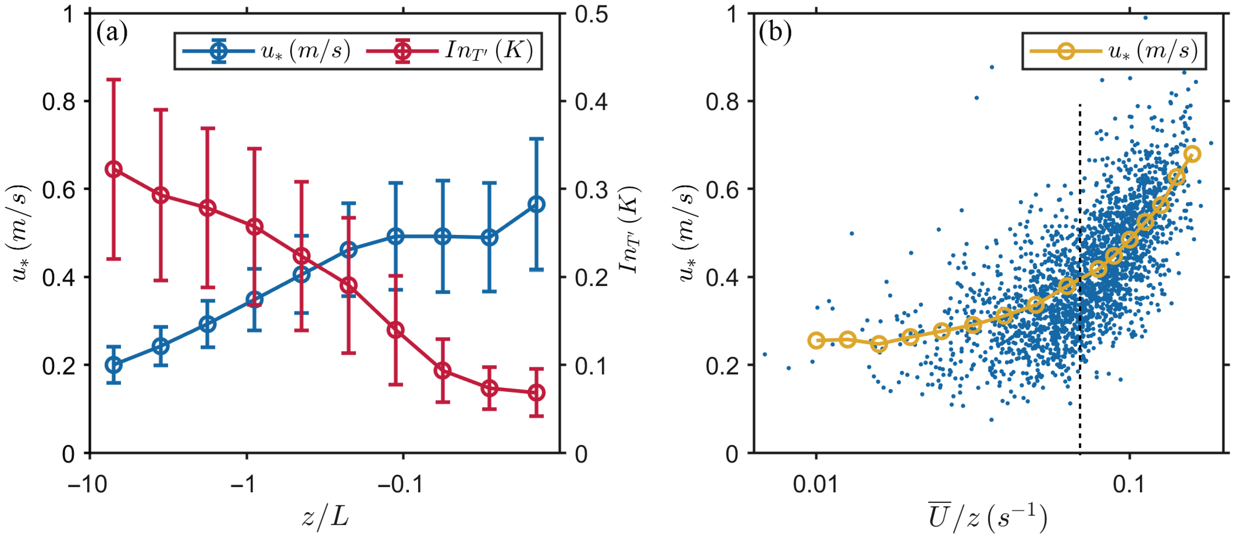
Wind shear-driven mechanical turbulence and buoyancy-driven thermal turbulence are represented by $u_{*}={({\overline{u^{\prime }{w}^{\prime }}}^2+{\overline{v\prime w\prime }}^2)}^{1/4}$ and temperature fluctuation intensity ${In}_{T^{\prime }}$, respectively, to quantify the contributions of wind shear and buoyancy under different stability conditions, as shown in Figure 4a. Note that $u_{*}$ represents the half-hour intensity of momentum flux observed at the measurement height $z$, and it should not be confused with friction velocity, which would typically be observed near the surface. The fluctuation intensity ${In}_{T^{\prime }}$ is calculated as the mean value of the fluctuations during half-hour large ejection and sweep motions. The relationship between $u_{*}$ (turbulence kinetic energy-related variables) and mean wind speed $\overline{U}=\sqrt{{\overline{u}}^2+{\overline{v}}^2}$ is shown in Figure 4b.

In Figure 4a, under neutral conditions, the intensity of $u_{*}$ is significantly higher, while the temperature fluctuation intensity is weak, reflecting strong wind shear and weak buoyancy. In contrast, under unstable conditions, $u_{*}$ weakens and ${In}_{T^{\prime }}$ enhances, indicating the dominant influence of buoyancy.

In Figure 4b, under low wind conditions, the dependence of $u_{\mathrm{*}}$ on $\overline{U}$ is minimal. However, as the wind speed increases, $u_{\mathrm{*}}$ exhibits a linear relationship with $\overline{U}$ under strong wind conditions. The pattern of $u_{\mathrm{*}}$ as a function of $\overline{U}$ resembles the shape of a hockey stick, consistent with the findings of Sun et al. [20]. The large $u_{\mathrm{*}}$ associated with bulk wind shear ($\overline{U}/z$) corresponds to the large $u_{\mathrm{*}}$ under near-neutral conditions, as shown in Figure 4a. As stability approaches neutral conditions, $u_{\mathrm{*}}$ increases linearly with bulk wind shear. This linear relationship between $u_{\mathrm{*}}$ and bulk wind shear under strong wind conditions indicates the dominant influence of bulk wind shear in generating large, nonlocal eddies comparable in scale to the observation height [20]. Sun et al. [20] found that bulk wind shear ($\overline{U}/z$), rather than local vertical shear ($\partial \overline{U}/\partial z$), predominates in turbulence generation under neutral conditions, and these nonlocal large eddies significantly enhance the vertical transport of momentum and heat.

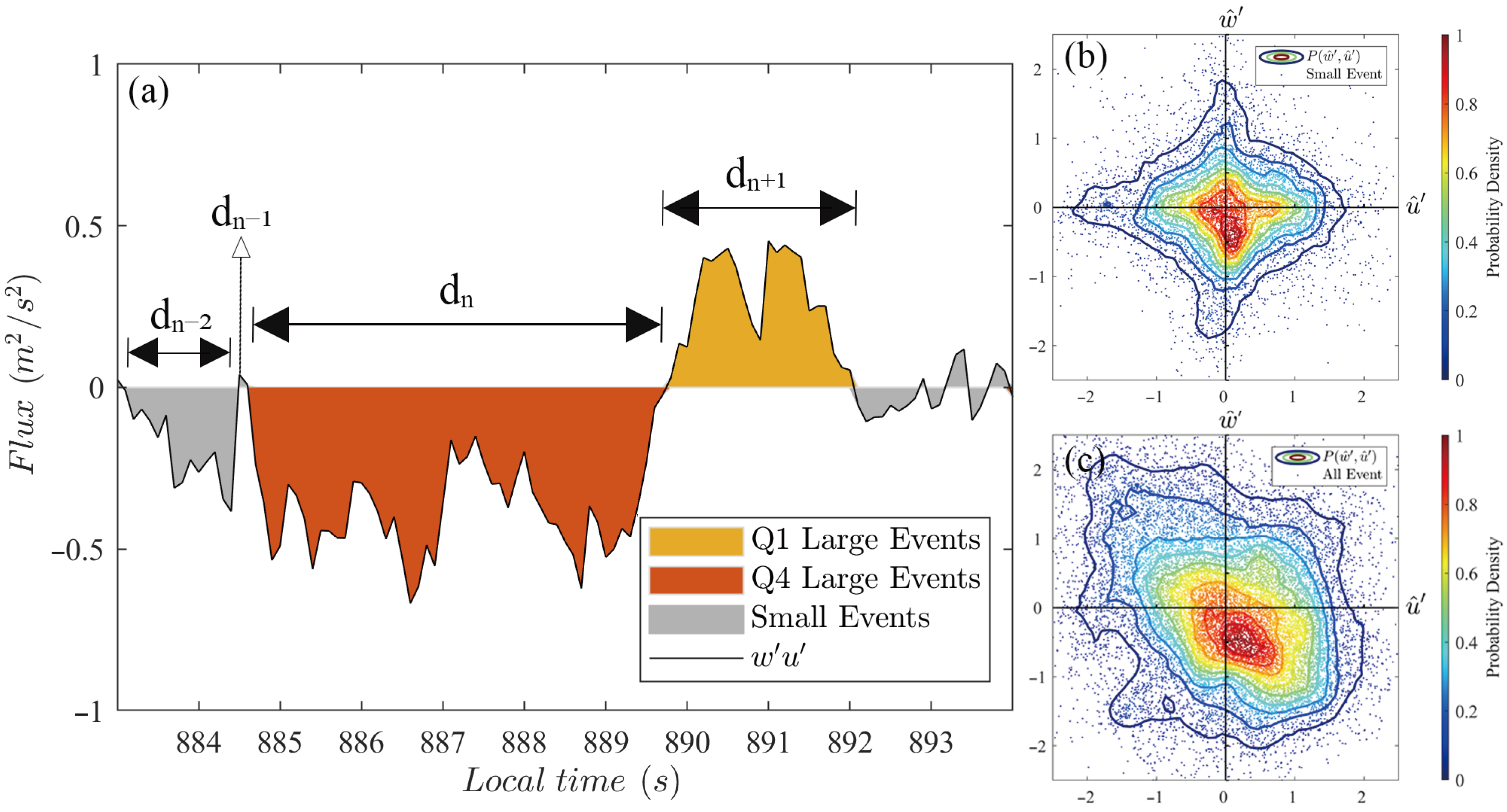
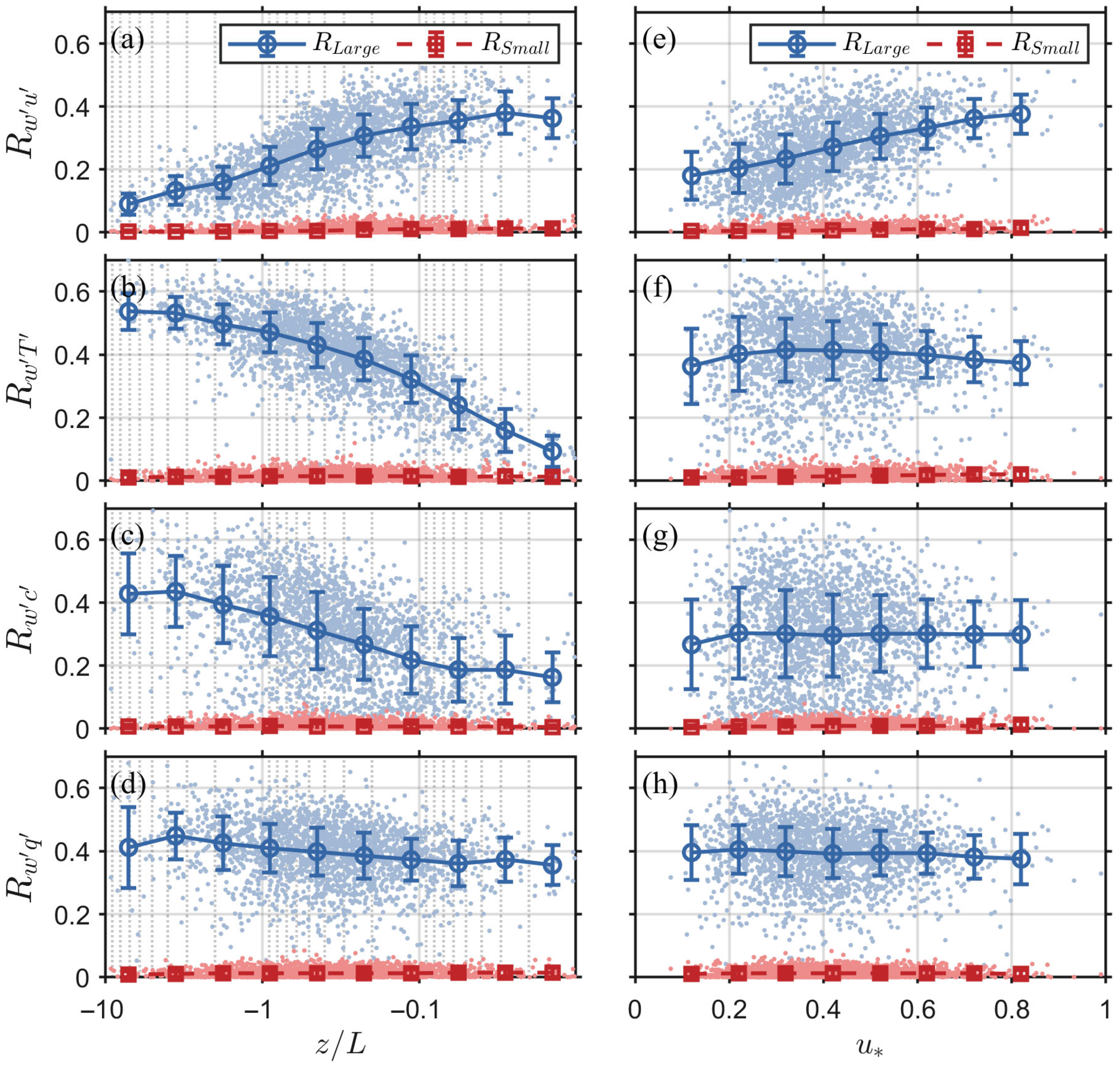
To further investigate the influence of buoyancy and wind shear on the transport of large turbulent events, we apply the quadrant analysis with a threshold $\tau$ to distinguish the large structures in the quadrants. These events contributed substantially to the overall flux, as shown in Table 1, despite occupying a relatively small fraction of the total time. The transfer efficiencies of the large and small events are characterized by calculating the correlation coefficients as follows:

$$R_{w^{\prime }{a}^{\prime },Large}=\left|{\displaystyle \frac{{\overline{w^{\prime }{a}^{\prime }}}_{Large events}}{{\sigma }_w{\sigma }_a}}\right|,$$

(9)

where ${\sigma }_w$ and ${\sigma }_a$ are the standard deviations of the vertical velocity $w$ and the turbulent component $a$, respectively. $R_{w^{\prime }{a}^{\prime }}$ represents the absolute value of the correlation between $w$ and $a$. ${\overline{w\prime a\prime }}_{Large events}$ denotes the mean flux from events with a duration $d>\tau$, whereas ${\overline{w\prime a\prime }}_{Small events}$ represents the mean flux from events with $d<\tau$.

Figure 5 illustrates the variations in the transfer efficiencies as a function of $u_{*}$ and $\zeta$. The transfer efficiencies of large events ($R_{Large}$) are significantly higher than those of small events ($R_{Small}$), indicating that the large events play a crucial role in the flux transport and effectively represent dominant eddies.

For momentum flux (Figure 5a,e), the correlation coefficients increase with stability approaching the neutral condition and with enhanced wind shear, suggesting that momentum flux transport is largely governed by wind shear intensity. In contrast, for heat flux (in Figure 5b), $R_{w^{\prime }{T}^{\prime }}$ is significantly influenced by the buoyancy-driven vertical motions under unstable conditions, whereas it decreases as buoyancy diminishes in neutral conditions. For passive scalars (water vapor and carbon dioxide), the correlation coefficients are also sensitive to buoyancy changes. However, in Figure 5f–h, correlation coefficients are insensitive to $u_{*}$ changes. The reason for this might be that the calculation reflects the correlation between $T\prime$ and $w^{\prime },$ rather than the absolute magnitude of the flux. As $u_{*}$ increases under near-neutral conditions, $w^{\prime }$ increases alongside the enhancement of vertical mixing, while the intensity of $T\prime$ decreases and the standard deviation of $T$ decreases, as shown in Figure 4a. This might lead to a stable correlation between $T\prime –w^{\prime }$, $c\prime –w^{\prime }$, and $q\prime –w^{\prime }$.

The observed decrease in the scalar flux transfer efficiencies as the stability approaches neutral conditions contrasts sharply with the increasing trend observed in the momentum flux. Similarly, the near-flat trend in scalar flux transfer efficiencies when wind shear intensifies is unlike the rising trend in the momentum flux transfer efficiencies. These dissimilarities between the scalars and momentum transport, which are consistent with the findings of Li and Bou-Zeid [3] and Schmutz and Vogt [7], highlight the influence of turbulent generation mechanisms under unstable conditions. Buoyancy primarily drives scalar transport, whereas wind shear enhances momentum transport.

Scalar transport related to the same eddies often exhibits different fluctuations owing to the independent sources and sinks of each scalar. To characterize the transport similarity between momentum, heat, and passive scalars, according to Li and Bou-Zeid [3], the correlation coefficients between $\overline{w^{\prime }{a}^{\prime }}$ and $\overline{w^{\prime }{b}^{\prime }}$ are calculated as

$$R_{w^{\prime }{a}^{\prime },w^{\prime }{b}^{\prime }}={\displaystyle \frac{\overline{\left(w^{\prime }{a}^{\prime }-\overline{w^{\prime }{a}^{\prime }}\right)\ast \left(w^{\prime }{b}^{\prime }-\overline{w^{\prime }{b}^{\prime }}\right)}}{{\sigma }_{w^{\prime }{a}^{\prime }}\ast {\sigma }_{w^{\prime }{b}^{\prime }}}},$$

(10)

where either $a’$ and $b’$ can be the turbulent fluctuating component $(u’, T’, q’, c’)$, ${\sigma }_{w^{\prime }{a}^{\prime }}$ and ${\sigma }_{w^{\prime }{b}^{\prime }}$ represents the standard deviations of $w^{\prime }{a}^{\prime }$ and $w^{\prime }{b}^{\prime }$, respectively. $w^{\prime }{a}^{\prime }$ is the original flux time series, and $\overline{w^{\prime }{a}^{\prime }}$ is the average flux of the 30 min period.

As shown in Figure 6a, under unstable conditions ($z/L<-1$), the correlation coefficients between the momentum and sensible heat fluxes are insignificant where turbulent motions are driven primarily by buoyancy and mechanical wind shear is relatively weak. The transport of momentum and passive scalars (${\mathrm{C}\mathrm{O}}_2$ and ${\mathrm{H}}_2\mathrm{O}$) is poorly correlated. The similarities between sensible heat and passive scalar transport are high (approximately 0.75), indicating that thermally driven turbulence predominates in the passive scalar transport under unstable conditions.

At the transition state between very unstable and neutral conditions ($-1<z/L<-0.1$), the momentum–heat transport is partially correlated, with absolute $R_{w^{\prime }{u}^{\prime },w^{\prime }{T}^{\prime }}$ approximately 0.4, where both buoyancy and wind shear affect the generation of large eddies.

Under near-neutral conditions ($z/L>-0.1$), bulk wind shear becomes significant, and the transport similarity between momentum and passive scalars increases, with $R_{w^{\prime }{u}^{\prime },w^{\prime }{q}^{\prime }}$ approximately 0.5 under neutral conditions. In Figure 6b, when the $u_{*}$ is high, the nonlocal large eddies generated by bulk wind shear significantly enhance the vertical turbulent mixing, increasing the transport similarities between momentum, heat, and passive scalars [8,22]. The nonlocal mixing of sensible heat flux weakens the temperature gradient, resulting in reduced buoyancy and a lower correlation between the momentum and sensible heat under near-neutral conditions. Moreover, the similarities between the sensible heat and passive scalars decrease as the influence of buoyancy diminishes. Under neutral conditions, the correlation coefficient of $R_{w^{\prime }{T}^{\prime },w^{\prime }{q}^{\prime }}$ is larger than $R_{w^{\prime }{T}^{\prime },w^{\prime }{c}^{\prime }}$, indicating that sensible heat and ${\mathrm{H}}_2\mathrm{O}$ are more strongly correlated than ${\mathrm{C}\mathrm{O}}_2$, since water vapor positively affects buoyancy. Additionally, the passive scalars are better correlated with the sensible heat flux (max $R_{w^{\prime }{T}^{\prime },w^{\prime }{q}^{\prime }}$ around 0.75 under unstable conditions) than with the momentum flux (max $R_{w^{\prime }{u}^{\prime },w^{\prime }{q}^{\prime }}$ around 0.5 under neutral conditions), indicating that buoyancy-driven turbulence transports passive scalars more efficiently than mechanically driven eddies.

Note that ${\mathrm{C}\mathrm{O}}_2$ has different profiles under neutral conditions in this dataset, owing to the different sinks and sources at 50 m height, which will be further discussed in Section 3.2. The general correlation coefficients results are consistent with those of prior studies [3,7,23], except for ${\mathrm{C}\mathrm{O}}_2$-related calculation under neutral conditions.

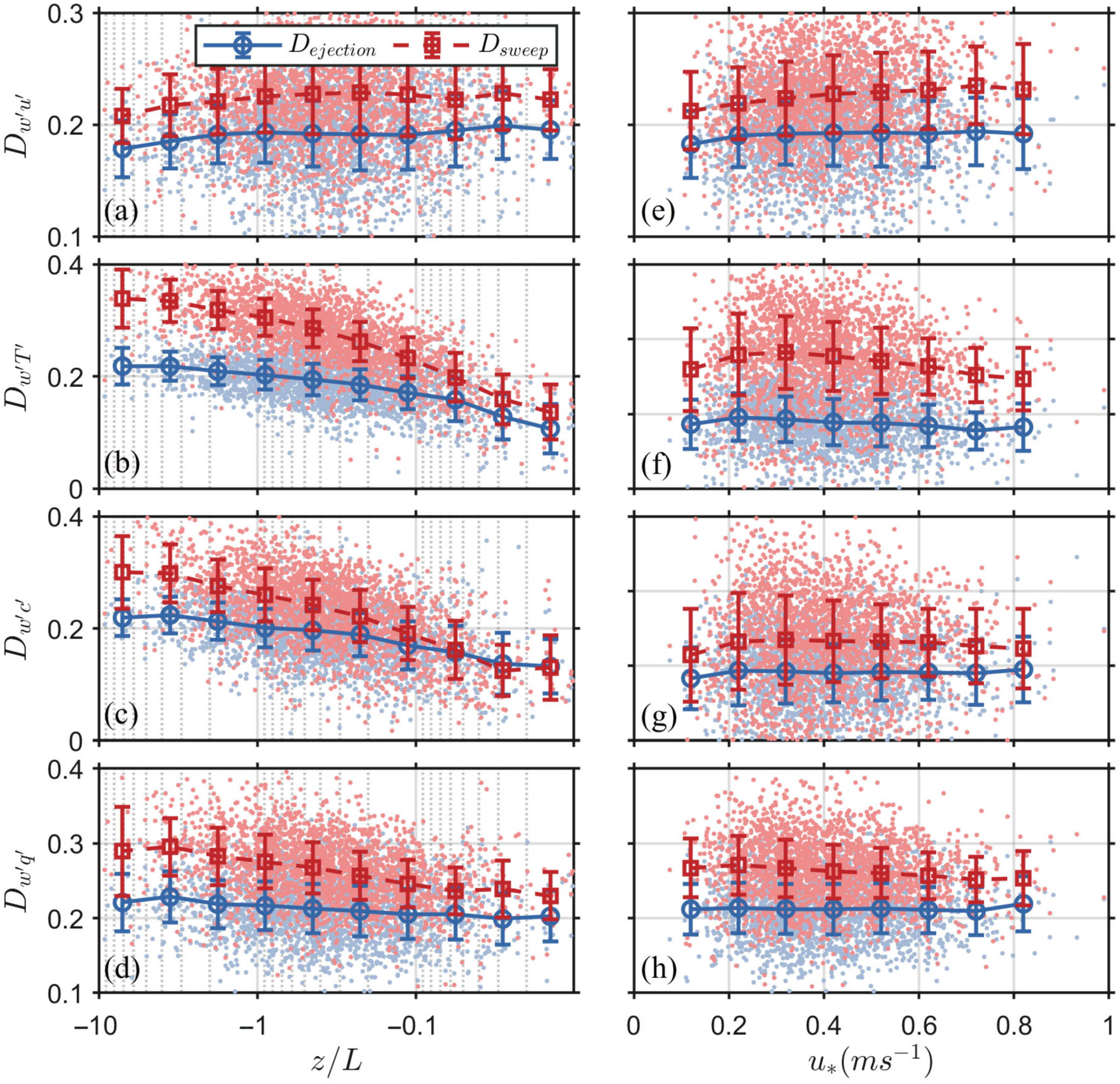
3.2. The Ejection and Sweep Behaviors Under Different Generation Mechanisms

To better understand how buoyancy and wind shear affect the flux transport dissimilarity, the ejections and sweeps are considered in separate calculations to characterize the impact of different turbulent generation mechanisms on the flux transport of large eddies. The intensity and duration of ejections and sweeps from large events selected by the threshold $\tau$ are calculated. The intensity is calculated as the mean value of the fluctuations during the ejection and sweep motions, as shown in Figure 7.

In Figure 7a–d, the trends in $u$-wind and scalar intensities vary distinctly with stability. The $u$-wind intensity exhibits an increasing trend towards neutral conditions, where wind shear dominates the generation of turbulence. In contrast, sensible heat and ${\mathrm{C}\mathrm{O}}_2$ intensities show decreasing trends owing to the lack of buoyancy and thermal gradients. ${\mathrm{H}}_2\mathrm{O}$, on the other hand, displays a trend that first increases and then decreases, indicating that the water vapor transport is influenced by both buoyancy and mechanically driven turbulence. These divergent behaviors between momentum and scalars are consistent with the flux transfer efficiencies shown in Figure 5, indicating that buoyancy and wind shear play different roles in influencing the intensity of large eddies in turbulent transport.

For the scalars, as shown in Figure 7b–d, the ejection intensity is higher than the sweep intensity under unstable conditions. This ejection–sweep asymmetry is caused by updrafts driven by buoyancy. When buoyancy diminishes and wind shear predominates in generating large eddies under neutral conditions, the well-mixed mechanical turbulent transport results in similar intensities of scalar ejections and sweeps.

For the $u$-wind, as shown in Figure 7a, the difference between ejection and sweep intensities are largely independent of stability changes, suggesting that buoyancy has no significant influence on $u$ wind intensity. In contrast, as shown in Figure 7e, the difference between ejection and sweep intensity increases as the wind shear strengthens, whereas the gap between the scalar ejection and sweep decreases as $u_{*}$ increases, as shown in Figure 7f–h.

Unlike the dissimilar trends between $u$-wind and the scalar intensities in the left panels, the increasing trends in all four fluctuations in the right panels highlight the dominant role of wind shear in enhancing large-eddy transport.

In conclusion, buoyancy significantly enhances the scalar ejection intensity, while wind shear boosts both ejection and sweep intensities in large eddies.

The mechanisms of large eddies can also be reflected in the durations of the ejection and sweep motions. Combined with the analysis of the flux-respective intensities in the previous discussion, the duration analysis offers deeper insights into the contributions of buoyancy and wind shear to transport processes in turbulent flow.

The durations $D_{i,L}$ of the momentum and scalar fluxes are determined by measuring the duration of large events occurring in the ejection and sweep quadrants, as shown in Figure 8. Under unstable conditions, as shown in Figure 8a, the variation in buoyancy has little effect on the momentum ejections and sweeps. The updrafts induced by buoyancy result in longer ejection durations for scalars (Figure 8b–d), highlighting the significant role of buoyancy in scalar flux transport. Sweep motions typically have longer durations than ejections, although ejections contribute more flux than sweeps [23], indicating that ejections are more efficient in transporting flux. Under neutral conditions, where buoyancy effects diminish, the ejection and sweep durations for the scalars tend to converge.

In Figure 8e–h, the durations of momentum and scalar ejections and sweeps are insensitive to changes in $u_{*}$. This indicates that mechanically driven turbulence has minimal influence on the duration of ejections and sweeps but enhances their flux intensity, as shown in Figure 7e–h. In contrast, buoyancy-driven turbulence affects both the duration and intensity of scalar ejections and sweeps. Under unstable conditions, buoyancy effects create more ejection and sweep motions, contributing to scalar flux transport.

The skewness of $u,w,T,c$, and $q$ are shown in Figure 9, illustrating the positive or negative deviations from the means of these fluctuations, specifically updrafts vs. downdrafts. For scalar fluctuations, absolute skewness values are larger under unstable conditions, indicating stronger updrafts than downdrafts. This asymmetry in ejections and sweeps is consistent with the patterns observed in Figure 7. The positive skewness of $w, q$ and $T$ under unstable conditions suggests that the buoyancy supports the warm and moist updrafts, corroborating findings of Li and Bou-Zeid [3]. Under neutral conditions, the scalar skewness values approach zero, reflecting well-mixed scalars and a more balanced ejection–sweep structure under strong wind shear. The skewness of ${\mathrm{C}\mathrm{O}}_2$ changes its sign under neutral conditions, indicating that the nonlocal vertical mixing driven by bulk wind shear introduces nonlocal sinks and sources and affects the ${\mathrm{C}\mathrm{O}}_2$ gradient at 50 m height.

In contrast to scalar fluctuations, the skewness of $u$-wind increases with enhanced wind shear, whereas $u$-wind skewness remains near zero under unstable conditions. The skewness of $w$ is consistently positive and decreases slightly under neutral conditions, but is insensitive to changes in $u_{*}$. This indicating that updrafts driven by both buoyancy and wind shear are stronger than downdrafts, and that ejection motions play a crucial role in turbulent transport. Wind shear predominantly enhances the asymmetry of $u$-wind towards negative values, whereas $w$-wind asymmetry remains positive, highlighting intensified ejection motions. As shown in Figure 8e, the duration of the ejection events is insensitive to $u_{*}$, suggesting that the efficiency of ejection flux transport is significantly enhanced.

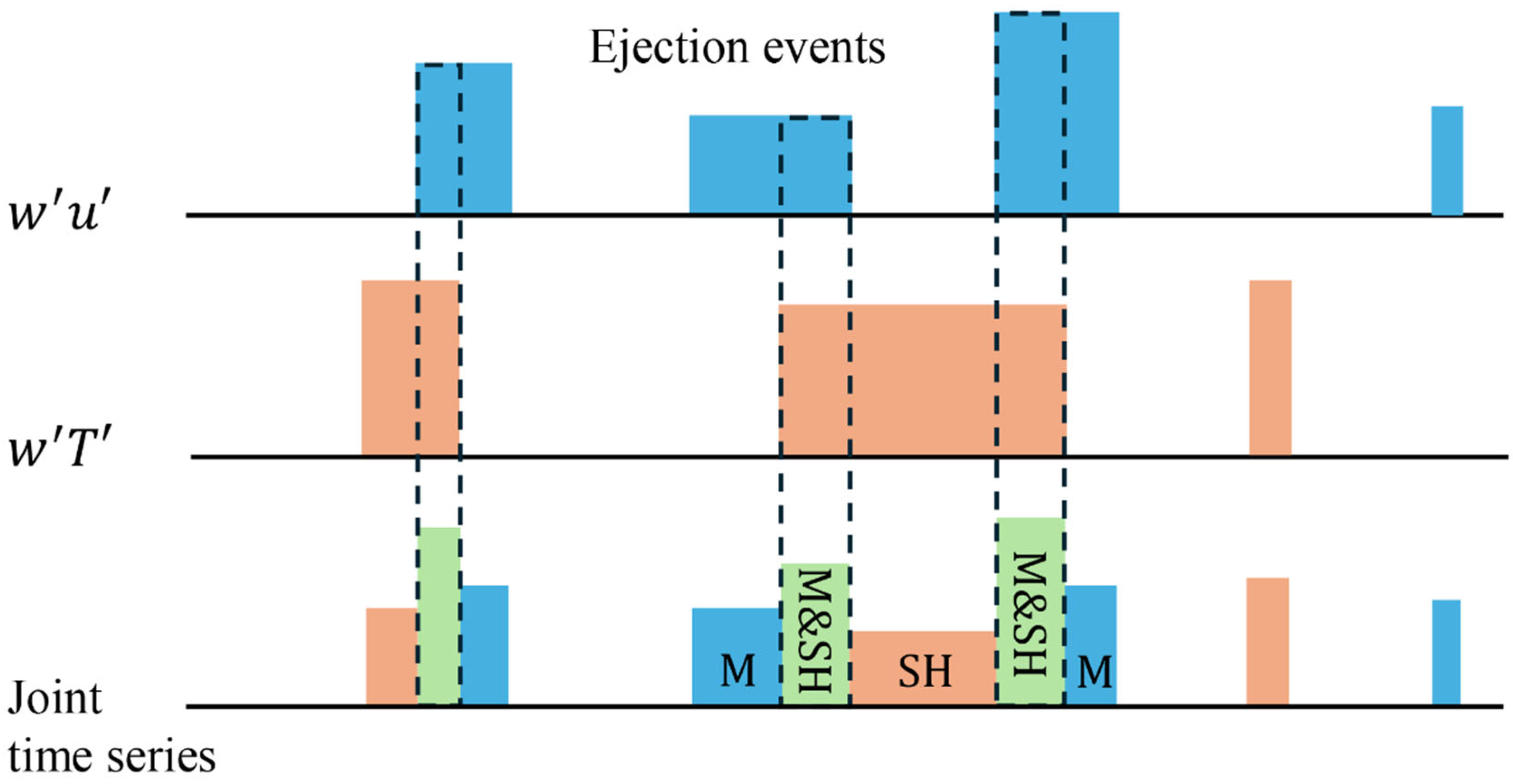
3.3. The Solo and Joint Flux Transport Between Momentum and Sensible Heat Fluxes

In this section, the influence of buoyancy and mechanically driven turbulence on flux transport is further investigated by analyzing the independent and synchronized transport of momentum and sensible heat flux. In a half-hour run, the momentum and heat ejections and sweeps in the time series can be classified as the solo transport of momentum ($M$), the solo transport of sensible heat ($SH$), and their joint transport ($M\&SH$), as shown in Figure 10.

In Figure 10, the ejection events on the joint time series are split into segments of solo flux (momentum or sensible heat) and joint transport between these fluxes. Every ejection or sweep event from momentum or sensible heat is compatible with these flux transport states. The durations of solo and joint flux transport are calculated as follows:

$$D_M={\displaystyle \frac{\sum momentum solo transport moments}{N}},$$

(11)

where $D_M$ represents the occurrence of solo momentum transport in the ejection and sweep events, and $D_{SH}$ (sensible heat transport) and $D_{M\&SH}$ (joint transport) are calculated similarly. In this section, ejections and sweeps are calculated as a whole because of their similar trends and sensitivities to stability changes.

As shown in Figure 6, the correlation coefficients between the momentum and sensible heat fluxes are relatively low under very unstable or neutral conditions, which matches the long duration for solo heat transport under unstable conditions and long duration for solo momentum transport under neutral conditions. These findings indicate that solo flux transport plays a significant role in influencing momentum and sensible heat dynamics.

Under unstable conditions ($z/L<-1$), as shown in Figure 11, the duration of solo sensible heat transport is equivalent to the joint transport of momentum and sensible heat fluxes and is significantly longer than the solo momentum transport. This indicates that thermal plumes and buoyancy generated large eddies that facilitate the joint transport of momentum and heat, whereas the mechanically driven turbulence is weak. Under neutral conditions, bulk wind shear weakens the temperature gradient, reducing the sensible heat flux transport while increasing momentum flux transport. The reduced temperature gradient also lowers buoyancy and diminishes heat flux-related transport activities, including both solo sensible heat flux and joint flux transport.

During the transition state between very unstable and neutral conditions ($-1<z/L<-0.1$), the solo sensible heat flux transport steadily declines as stability increases, indicating that the thermal gradient force continuously decreases. Near $z/L=-0.1$, the duration of solo momentum transport exceeds that of the solo sensible heat flux transport. This reflects the more frequent occurrence of mechanically driven turbulence compared with buoyancy-driven turbulence, indicating that wind shear plays a dominant role over buoyancy.

The relatively flat trend in the joint flux transport under unstable conditions might be explained by the offsetting effects of increasing shear-generated turbulence and decreasing buoyancy. The near-flat trend in the solo momentum transport indicates that most of the mechanically generated turbulence develops locally [8,21]. As wind shear is enhanced under unstable conditions, local mechanical turbulence activities are primarily generated within buoyancy-driven structures, such as thermal plumes. Another way to understand this is that buoyancy predominates in the surface layer, where the most turbulent changes occur under its influence. This development also increases the co-transport with sensible heat flux, corroborating the increasing momentum–heat transport similarity under the transition state shown in Figure 6. The increase–decrease offsetting and local developing result in a steady duration for co-transport events despite stability changes.

A noticeable slope change in solo momentum transport under near neutral conditions ($z/L>-0.1$) indicates the significant development of nonlocal mechanically generated turbulence as wind shear continuously enhances. As the local mechanically driven turbulence becomes nonlocal, the structural stability of local thermal plumes diminishes, resulting in a decrease in the occurrence of joint flux transport occurrence events.

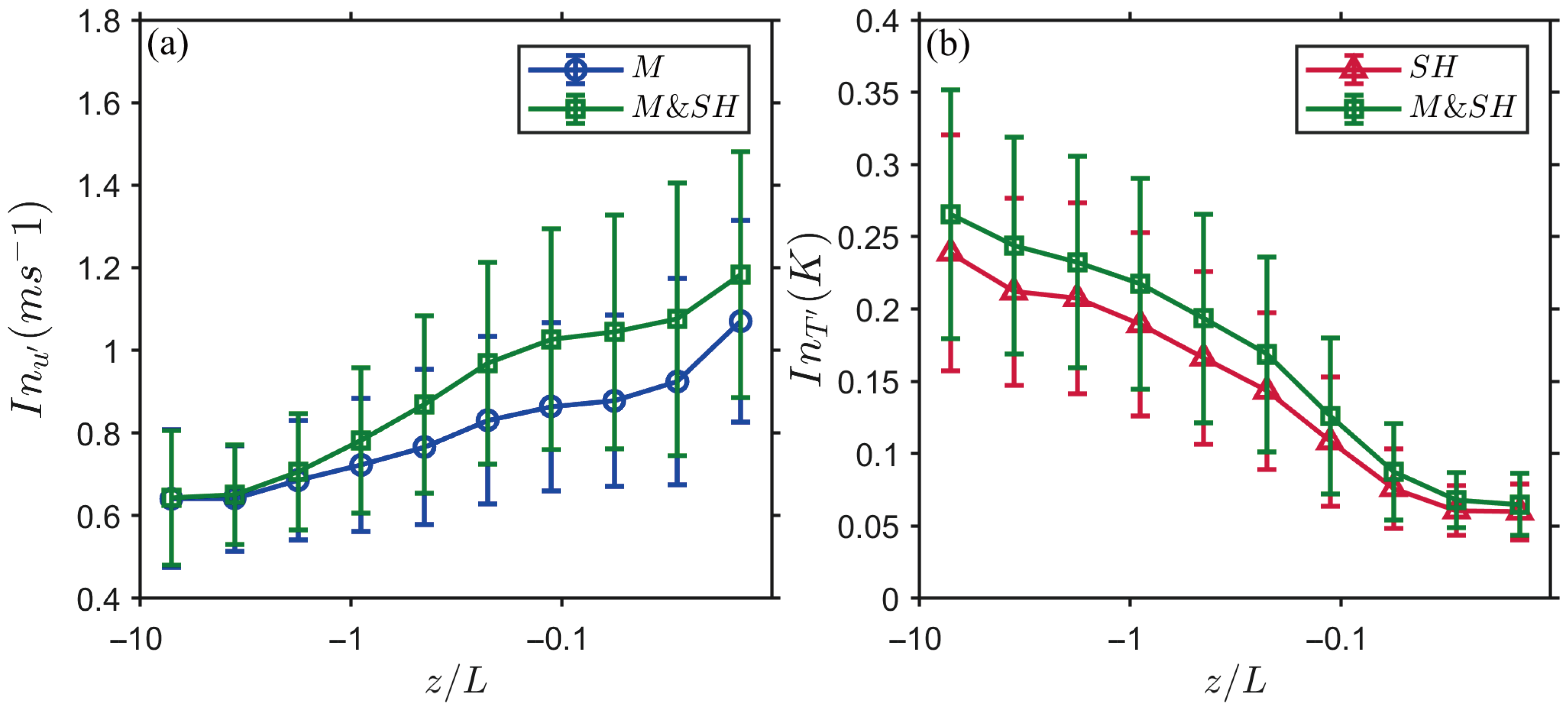
The average fluctuation intensities of $u’$ and $T’$ during solo and joint transport process are calculated and are shown in Figure 12. The $u’$ intensity increases as the wind shear increases, whereas $T’$ intensity decreases as buoyancy diminishes.

Under neutral conditions, the lack of strong buoyancy forces indicates that both solo heat and joint transport events are influenced similarly by wind shear, leading to similar fluctuation intensities of $T’$. Under unstable conditions, the strong vertical motions driven by buoyancy leads to similar $u’$ intensities for the solo and co-transport events.

The intensity of joint transport is higher than that of solo transport. Under near-neutral conditions, the combined transport of momentum and heat driven by wind shear is more efficient in turbulent mixing and transport, leading to high velocity fluctuation intensities during joint transport events. Under unstable conditions, co-transport events benefit from the combined effects of buoyancy and wind shear, resulting in high temperature fluctuation. Solo sensible heat flux transport shows low intensities owing to the lack of this synergistic effect.

The slope of the fluctuation intensity $u’$ during joint transport increases faster than that during momentum transport under unstable conditions ($z/L<-0.1$), as shown in Figure 12a. This indicates that local mechanically driven turbulence is more developed within buoyancy-driven structures than when influenced solely by wind shear. This finding aligns with the previous discussion, in which local mechanically driven turbulence is primarily generated with buoyancy-driven structures. Under near-neutral conditions ($z/L>-0.1$), the increasing trends in solo and joint transport become similar, indicating that nonlocal shear-generated turbulence predominates the solo and joint flux transport. Conversely, for $T’$ intensity, a similar decreasing trend in both solo and joint flux transport under unstable conditions reflects the dominant role of buoyancy despite its decrease.

The dynamics between these mechanisms can be further investigated using passive scalars. The fluctuation intensity of ${\mathrm{H}}_2\mathrm{O}$ in solo and joint transport is calculated, as shown in Figure 13. Note that ${\mathrm{C}\mathrm{O}}_2$ intensity is not discussed here because of its different profile compared to those in prior studies, as shown in Figure 9.

Under unstable conditions, buoyancy dominates ${\mathrm{H}}_2\mathrm{O}$ transport, leading to higher ${\mathrm{H}}_2\mathrm{O}$ fluctuation intensities during joint transport and solo heat transport than during solo momentum transport. In joint transport events, ${\mathrm{H}}_2\mathrm{O}$ is under the combined influence of wind shear and buoyancy, resulting in high intensities.

Under near-neutral conditions, the intensities during solo momentum transport are higher than those during solo heat transport, indicating the dominant role of shear-generated turbulence. The correlation between ${\mathrm{H}}_2\mathrm{O}$ and momentum fluxes is significantly lower than that between ${\mathrm{H}}_2\mathrm{O}$ and sensible heat, as shown in Figure 6. Additionally, ${\mathrm{H}}_2\mathrm{O}$ has a positive effect on buoyancy [7]. This results in small intensity differences between the solo momentum and solo heat transport. In joint transport events, turbulent mixing is more effective for transporting both momentum and heat fluxes, leading to the high transport efficiency of ${\mathrm{H}}_2\mathrm{O}$.

A noticeable slope change can be found near $z/L=-0.1$, where wind shear and buoyancy are equally matched, resulting in the highest intensity of ${\mathrm{H}}_2\mathrm{O}$ during joint transport events, which is consistent with the intensity result from Figure 7d. Under unstable conditions, the ${\mathrm{H}}_2\mathrm{O}$ intensity during the solo heat flux transport increases as the stability approaches neutral conditions. In the discussion in Section 3.1, the reason for the increasing trend under unstable conditions is the combined influence of wind shear and buoyancy. When only the influence of buoyancy is considered, this may be explained by the fact that, under very unstable conditions, low wind speed and high temperature gradients cause rapid water loss from plants, prompting them to close their stomata to conserve water. Therefore, the decrease in plant transpiration and photosynthesis weakens water vapor gradient and transport. As the wind shear increases and thermal gradient weakens, the evaporation rate from the plants increases. The dissimilarity changes between the sources and sinks of heat and water vapor results in different vertical turbulent transport, corroborating the results of previous studies [9,11,16,28].

4. Discussion

We have utilized four years of EC data collected at 50 m above a complex suburban canopy to analyze the influence of buoyancy and wind shear on transport similarity in an unstable ABL. The quadrant analysis method with a time threshold $\tau$ is employed to identify the small isotropic flux events within four quadrants. By eliminating these small events from each data run, we focus on analyzing large eddies, which are more efficient at transporting fluxes than that of isotropic small events.

The transfer efficiency results show that large events play a crucial role in flux transport and represent the dominant eddies well. The momentum transfer efficiencies increase with increasing wind shear, whereas the scalars’ transfer efficiencies are mostly influenced by buoyancy changes. This indicates that buoyancy-driven turbulence primarily drives scalar transport, whereas mechanically driven turbulence enhances momentum transport. The correlation coefficients for all combinations of the measured fluxes are calculated to further demonstrate the different interactions between momentum and the scalars during turbulent transport. The enhanced wind shear increases both the momentum–scalar and scalar–scalar correlations, indicating that well-mixed turbulence generated by bulk wind shear improves co-transport between fluxes. Strong buoyancy significantly enhances the correlation between scalar transport, while the momentum–scalar transport dissimilarity increases. Passive scalars are more correlated to buoyancy-driven turbulence than mechanically driven motions.

Moreover, buoyancy primarily enhances the scalars’ intensity and the occurrence of ejection, creating both intensity and duration asymmetries between the ejections of scalars and sweeps. In contrast, wind shear amplifies both the ejection and sweep intensities for all turbulent fluctuating components, primarily for $u’$, while having a low influence on the ejection–sweep durations. The skewness of $u$ and $w$ shows the dominance of ejection motions within large eddies, while the skewness of the scalars reflects the substantial impact of buoyancy on ejections under unstable conditions and well-mixed transport under wind shear dominance. These findings corroborate those of Li and Bou-Zeid [3], except for the ${\mathrm{C}\mathrm{O}}_2$ profile under neutral conditions owing to nonlocal sinks and sources.

The dynamics between the buoyancy and mechanically driven turbulence have been further investigated with the decomposition of the solo and joint transport between the momentum and sensible heat flux. The results indicate that wind shear dominates the solo momentum transport period and buoyancy dominates the solo heat flux transport period. Under unstable conditions, the offsetting effects of the increasing shear-generated turbulence and decreasing buoyancy maintain the occurrence of co-transport events insensitive to stability changes. Local shear-generated turbulence primarily develops within buoyancy-driven turbulence, resulting in an increase in momentum–heat transport similarity. Under near-neutral conditions, nonlocal large eddies driven by bulk wind shear weaken buoyancy structures, leading to a decrease in joint transport events. Moreover, the intensity of the joint transport is under the combined influence of buoyancy and wind shear, resulting in a high fluctuation intensity for velocity, temperature, and water vapor. When stability shifts from unstable to neutral, the enhancement of plant transpiration and photosynthesis, driven by increased wind speed and a weakening temperature gradient, creates distinctly different local sources and sinks between sensible heat and water vapor. This leads to a different intensity trend for the water vapor intensity compared with sensible heat flux. When nonlocal eddies dominate, the water vapor transport driven by sensible heat diminishes, reflecting the contrasting roles of local and nonlocal processes.

In conclusion, this study investigates the influence of turbulence generation mechanisms on large-scale turbulent structures and their flux transport characteristics. By analyzing the independent and synchronized transport of momentum and heat, the study clearly reveals the dynamics between nonlocal and local turbulent eddies. Additionally, evidence of changes in water vapor sources and sinks under low-wind and high-heat conditions is identified, which requires further validation and analysis with additional observational data.

References

1. Steiner, A.L.; Pressley, S.N.; Botros, A.; Jones, E.; Chung, S.H.; Edburg, S.L. Analysis of Coherent Structures and Atmosphere-Canopy Coupling Strength During the Cabinex Field Campaign. Atmos. Chem. Phys. 2011, 11, 11921–11936. [Google Scholar] [CrossRef]
2. Finnigan, J.J.; Shaw, R.H.; Patton, E.G. Turbulence Structure above a Vegetation Canopy. J. Fluid Mech. 2009, 637, 387–424. [Google Scholar] [CrossRef]
3. Li, D.; Elie, B.-Z. Coherent Structures and the Dissimilarity of Turbulent Transport of Momentum and Scalars in the Unstable Atmospheric Surface Layer. Bound.-Layer Meteorol. 2011, 140, 243–262. [Google Scholar] [CrossRef]
4. Choi, T.; Hong, J.; Kim, J.; Lee, H.; Asanuma, J.; Ishikawa, H.; Tsukamoto, O.; Zhiqiu, G.; Ma, Y.; Ueno, K.; et al. Turbulent Exchange of Heat, Water Vapor, and Momentum over a Tibetan Prairie by Eddy Covariance and Flux Variance Measurements. J. Geophys. Res. Atmos. 2004, 109, D21106. [Google Scholar] [CrossRef]
5. Larsén, X.G.; Kelly, M.; Sempreviva, A.M. On the Temperature and Humidity Dissimilarity in the Marine Surface Layer. Bound.-Layer Meteorol. 2014, 151, 273–291. [Google Scholar] [CrossRef]
6. Gao, Z.; Liu, H.; Li, D.; Katul, G.G.; Blanken, P.D. Enhanced Temperature-Humidity Similarity Caused by Entrainment Processes with Increased Wind Shear. J. Geophys. Res. Atmos. 2018, 123, 4110–4121. [Google Scholar] [CrossRef]
7. Schmutz, M.; Vogt, R. Flux Similarity and Turbulent Transport of Momentum, Heat and Carbon Dioxide in the Urban Boundary Layer. Bound.-Layer Meteorol. 2019, 172, 45–65. [Google Scholar] [CrossRef]
8. Lan, C.; Wang, B.; Zheng, D.; Wang, Y.; Zhang, Z.; Fang, R. Decreased Dissimilarity of Turbulent Transport Attributed to Large Eddies. Q. J. R. Meteorol. Soc. 2022, 148, 1262–1279. [Google Scholar] [CrossRef]
9. Katul, G.; Goltz, S.M.; Hsieh, C.I.; Cheng, Y.; Mowry, F.; Sigmon, J. Estimation of Surface Heat and Momentum Fluxes Using the Flux-Variance Method above Uniform and Non-Uniform Terrain. Bound.-Layer Meteorol. 1995, 74, 237–260. [Google Scholar] [CrossRef]
10. De Bruin, H.A.R.; Van Den Hurk, B.J.J.M.; Kroon, L.J.M. On the Temperature-Humidity Correlation and Similarity. Bound.-Layer Meteorol. 1999, 93, 453–468. [Google Scholar] [CrossRef]
11. Williams, C.A.; Scanlon, T.M.; Albertson, J.D. Influence of Surface Heterogeneity on Scalar Dissimilarity in the Roughness Sublayer. Bound.-Layer Meteorol. 2006, 122, 149–165. [Google Scholar] [CrossRef]
12. Assouline, S.; Tyler, S.W.; Tanny, J.; Cohen, S.; Bou-Zeid, E.; Parlange, M.B.; Katul, G.G. Evaporation from Three Water Bodies of Different Sizes and Climates: Measurements and Scaling Analysis. Adv. Water Resour. 2008, 31, 160–172. [Google Scholar] [CrossRef]
13. Sempreviva, A.M.; Højstrup, J. Transport of Temperature and Humidity Variance and Covariance in the Marine Surface Layer. Bound.-Layer Meteorol. 1998, 87, 233–253. [Google Scholar] [CrossRef]
14. Lan, C.; Liu, H.; Li, D.; Katul, G.G.; Finn, D. Distinct Turbulence Structures in Stably Stratified Boundary Layers with Weak and Strong Surface Shear. J. Geophys. Res. Atmos. 2018, 123, 7839–7854. [Google Scholar] [CrossRef]
15. Mahrt, L. Boundary-Layer Moisture Regimes. Q. J. R. Meteorol. Soc. 2006, 117, 151–176. [Google Scholar]
16. Shaw, R.H.; Tavangar, J.; Ward, D.P. Structure of the Reynolds Stress in a Canopy Layer. J. Clim. Appl. Meteorol. 1983, 22, 1922–1931. [Google Scholar] [CrossRef]
17. Robinson, S.K. Coherent Motions in the Turbulent Boundary Layer. Annu. Rev. Fluid Mech. 1991, 23, 601–639. [Google Scholar] [CrossRef]
18. Katul, G.; Hsieh, C.I.; Kuhn, G.; Ellsworth, D.; Nie, D. Turbulent Eddy Motion at the Forest-Atmosphere Interface. J. Geophys. Res. Atmos. 1997, 102, 13409–13421. [Google Scholar] [CrossRef]
19. Katul, G.G.; Sempreviva, A.M.; Cava, D. The Temperature–Humidity Covariance in the Marine Surface Layer: A One-Dimensional Analytical Model. Bound.-Layer Meteorol. 2007, 126, 263–278. [Google Scholar] [CrossRef]
20. Sun, J.; Takle, E.S.; Acevedo, O.C. Understanding Physical Processes Represented by the Monin–Obukhov Bulk Formula for Momentum Transfer. Bound.-Layer Meteorol. 2020, 177, 69–95. [Google Scholar] [CrossRef]
21. Sun, J.; Lenschow, D.H.; LeMone, M.A.; Mahrt, L. The Role of Large-Coherent-Eddy Transport in the Atmospheric Surface Layer Based on Cases-99 Observations. Bound.-Layer Meteorol. 2016, 160, 83–111. [Google Scholar] [CrossRef]
22. Wang, Y.; Wang, B.; Lan, C.; Fang, R.; Zheng, B.; Lu, J.; Zheng, D. Improved Quadrant Analysis for Large-Scale Events Detection in Turbulent Transport. Atmosphere 2022, 13, 489. [Google Scholar] [CrossRef]
23. Lan, C.; Wang, B.; Li, L.; Fang, R.; Wang, Y.; Zhang, Z.; Zheng, B. Linkage between Surface Energy Balance Non-Closure And horizontal Asymmetric Turbulent Transport. Q. J. R. Meteorol. Soc. 2023, 149, 3383–3400. [Google Scholar] [CrossRef]
24. Foken, T.; Mathias, G.; Matthias, M.; Larry, M.; Brian, A.; William, M. Post-Field Data Quality Control. In Handbook of Micrometeorology; Springer: Dordrecht, The Netherlands, 2005; pp. 181–208. [Google Scholar]
25. Kaimal, J.C.; Wyngaard, J.C.J.; Izumi, Y.; Coté, O.R. Spectral Characteristics of Surface-Layer Turbulence. Q. J. R. Meteorol. Soc. 2006, 98, 563–589. [Google Scholar]
26. Fortuniak, K.; Włodzimierz, P. Selected Spectral Characteristics of Turbulence over an Urbanized Area in the Centre of Łódź, Poland. Bound.-Layer Meteorol. 2014, 154, 137–156. [Google Scholar] [CrossRef]
27. Lu, S.S.; Willmarth, W.W. Measurements of the Structure of the Reynolds Stress in a Turbulent Boundary Layer. J. Fluid Mech. 2006, 60, 481–511. [Google Scholar] [CrossRef]
28. Lee, X.; Yu, Q.; Sun, X.; Liu, J.; Min, Q.; Liu, Y.; Zhang, X. Micrometeorological Fluxes under the Influence of Regional and Local Advection: A Revisit. Agric. For. Meteorol. 2004, 122, 111–124. [Google Scholar] [CrossRef]
Figure 1. (a) A topographic map of Zengcheng station (orange rectangle) and the observation tower (red spot) from Google Earth. The subplot at the top left displays a Google Earth image of the observation site in Zengcheng, Guangdong Province. The subplot at bottom right shows a photograph of the flux observation tower, with a red indicating the observation height. (b) The wind-rose diagram of selected 30 min runs. (c) The number of selected runs in each hour during 8 : 00 20 : 00 local time.
Atmosphere 15 01266 g001
Figure 2. Normalized vertical velocity spectra S w are plotted against the non-dimensional frequency f = n z / U ¯ . The colored lines indicate different stability categories and the short dashed black line indicates the 2 / 3 slope.
Atmosphere 15 01266 g002
Figure 3. (a) Flux–time series (black line), with red and yellow coloring, represents the large flux events ( d n > τ ) from different quadrants, while the small events with duration ( d n < τ ) are colored in gray. (b) A scatter plot of small events ( d n < τ ) and its probability density contour. (c) A scatter plot of all events (the original data) and its probability density contour.
Atmosphere 15 01266 g003
Figure 4. (a) The intensities of momentum flux u * (blue line, corresponding to the left Y-axis) and temperature fluctuation I n T (red line, corresponding to the right Y-axis) as functions of ζ . Markers with error bars represent the bin averages and the corresponding standard deviations of intensities. (b) u * (blue scatter) as a function of bulk wind shear U ¯ / z at the observation height ( z = 50 m). Yellow markers indicate the bin averages, and the vertical dashed line marks the point where u * and U ¯ / z exhibit a linear relationship.
Atmosphere 15 01266 g004
Figure 5. The transfer efficiencies of (a) momentum, (b) sensible heat, (c) carbon dioxide, and (d) water vapor as functions of ζ (left panels). The transfer efficiencies of (e) momentum, (f) sensible heat, (g) carbon dioxide, and (h) water vapor as functions of u * (right panels). The blue markers with error bars represent the bin averages and the corresponding standard deviations of large flux events, whereas the red markers with error bars depict the same for small flux events.
Atmosphere 15 01266 g005
Figure 6. (a) The transport similarity ( R w a , w b ) for all combinations of measured covariances as a function of ζ . (b) The transport similarity ( R w a , w b ) as a function of u * . The markers with error bars represent the bin averages and the corresponding standard deviations of the correlation coefficients.
Atmosphere 15 01266 g006
Figure 7. The intensity of (a) momentum, (b) sensible heat, (c) carbon dioxide, and (d) water vapor as functions of ζ (left panels). The intensity of (e) momentum, (f) sensible heat, (g) carbon dioxide, and (h) water vapor as functions of u * (right panels). The blue markers with error bars represent the bin averages and the corresponding standard deviations of ejection intensity, whereas the red markers with error bars depict the same for sweep intensity.
Atmosphere 15 01266 g007
Figure 8. Duration of (a) momentum, (b) sensible heat, (c) carbon dioxide, and (d) water vapor as functions of ζ (left panels). The duration of (e) momentum, (f) sensible heat, (g) carbon dioxide, and (h) water vapor as functions of u * (right panels). The blue markers with error bars represent the bin averages and the corresponding standard deviations of ejection duration, whereas the red markers with error bars depict the same for sweep duration.
Atmosphere 15 01266 g008
Figure 9. The skewness of fluctuations of (a) ζ and (b) u * . The blue ( u ), red ( T ), black ( c ), orange ( q ), and green ( w ) markers with error bars represent the bin averages and the corresponding standard deviations of skewness.
Atmosphere 15 01266 g009
Figure 10. A schematic representation of the ejection events’ time series of momentum flux (blue boxes), heat flux (yellow boxes), and their joint time series, where momentum and heat ejection events coincide (dashed boxes and green boxes) or occur individually.
Atmosphere 15 01266 g010
Figure 11. The duration of solo momentum flux (blue line), solo sensible heat flux (red line), and joint flux transport (green line) as functions of stability ζ . Markers with error bars represent the bin averages and the corresponding standard deviations of durations.
Atmosphere 15 01266 g011
Figure 12. (a) The average intensity of u during solo momentum flux (blue line) and joint flux transport (green line) as functions of stability ζ (left panel). (b) The average intensity of T during solo sensible heat flux (red line) and joint flux transport (green line) as functions of stability ζ . Markers with error bars represent the bin averages and the corresponding standard deviations of durations.
Atmosphere 15 01266 g012
Figure 13. The intensity of H 2 O during solo momentum flux (blue line), solo sensible heat flux (red line), and joint flux transport (green line) as functions of stability ζ . Markers with error bars represent the bin averages and the corresponding standard deviations of durations.
Atmosphere 15 01266 g013