
Microclimate Multivariate Analysis of Two Industrial Areas


Abstract
1. Introduction
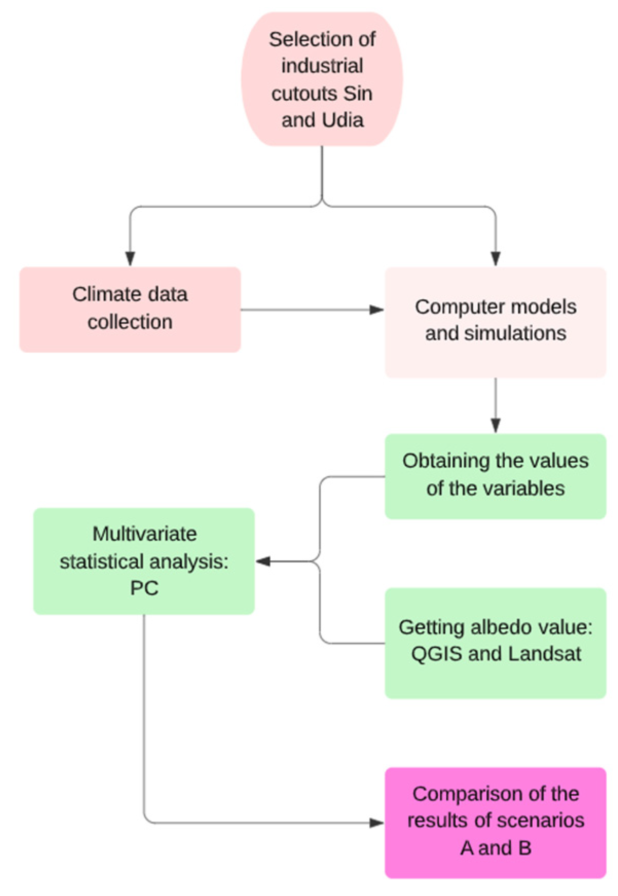
2. Methods
2.1. Input Parameters for ENVI-Met
2.2. Albedo Calculation
2.3. Multivariate Analysis
3. Results
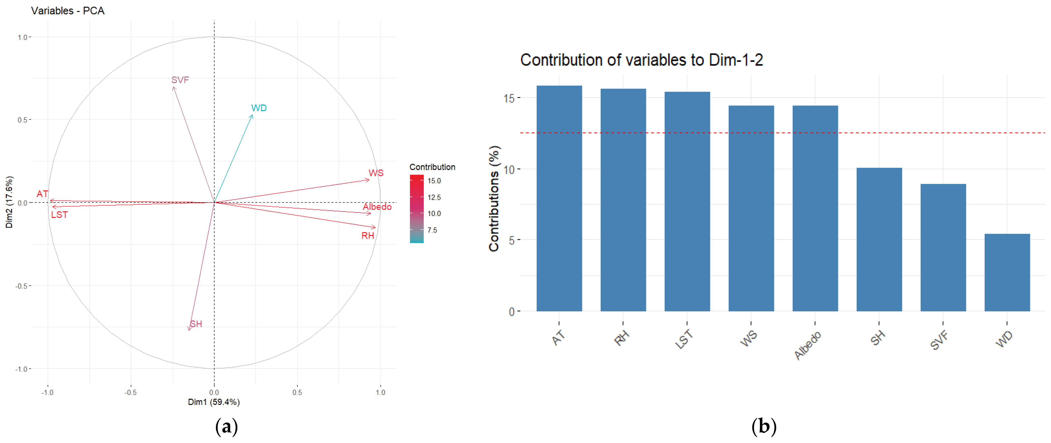
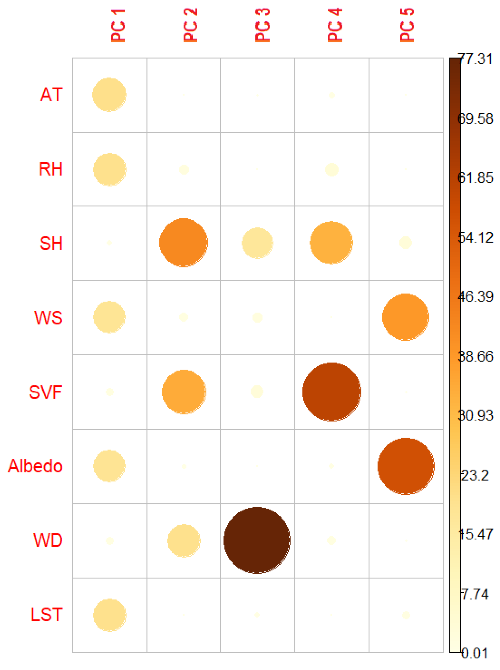
- Hierarchical clustering and principal component analysis (PCA): Assessment to reveal similarities in data distribution patterns and establish possible associations between the main variables in the microclimate study of each clipping and the impact of each variable for the scenario studied;
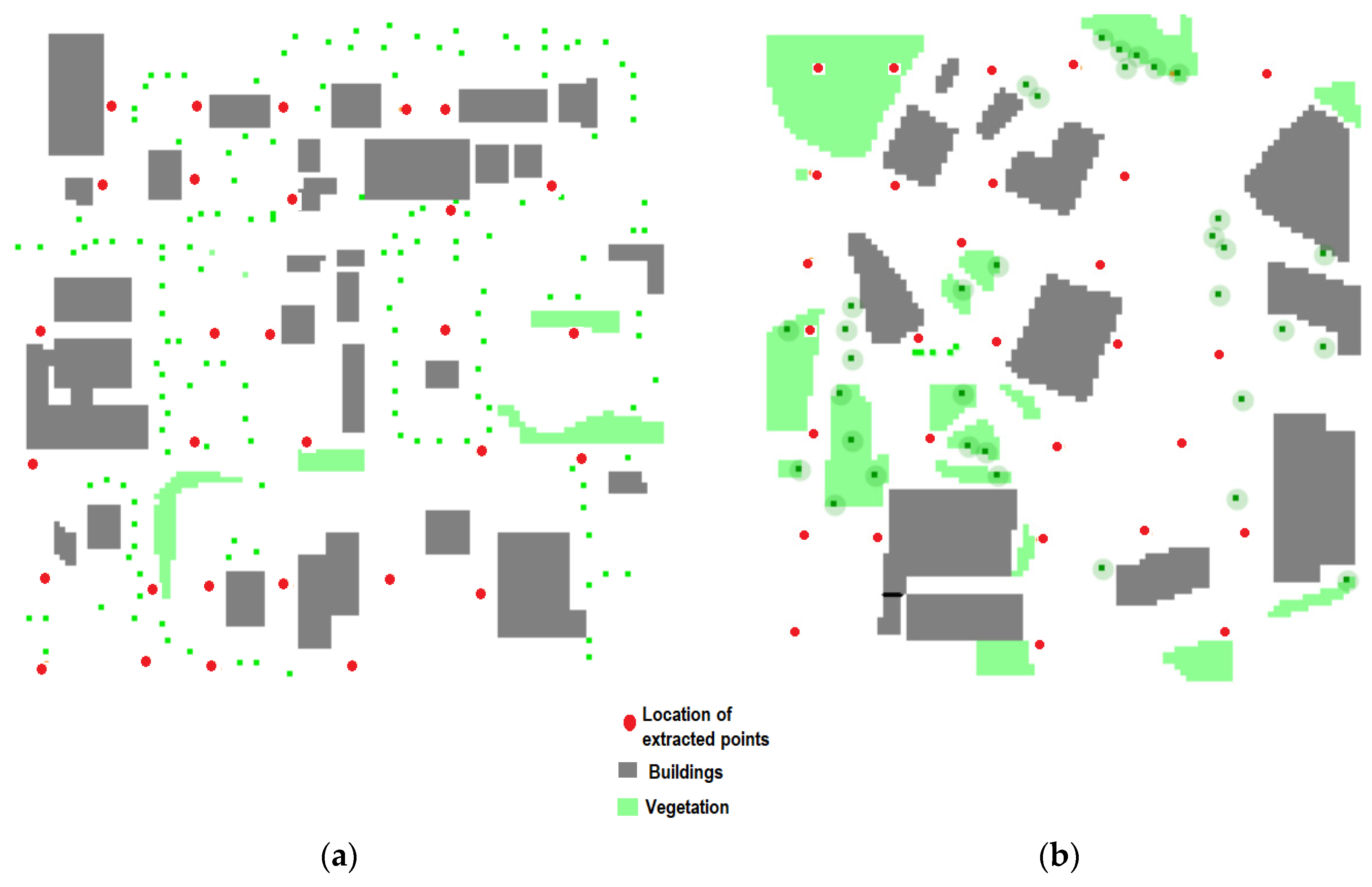
- Physical composition of the clippings and albedo: Presentation of the physical characterization and albedo of the clippings, which influence the urban microclimate;
- Descriptive analysis: Assessment of the simulation results for the variables with the greatest impact on each scenario.
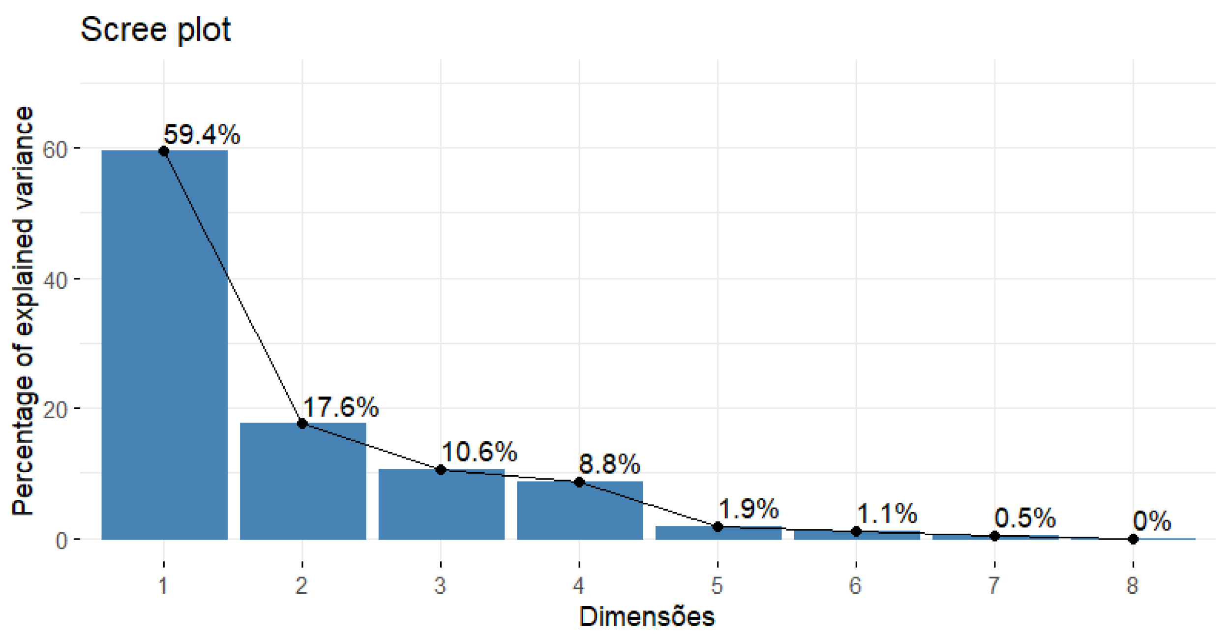
3.1. Hierarchical Clustering and Principal Component Analysis
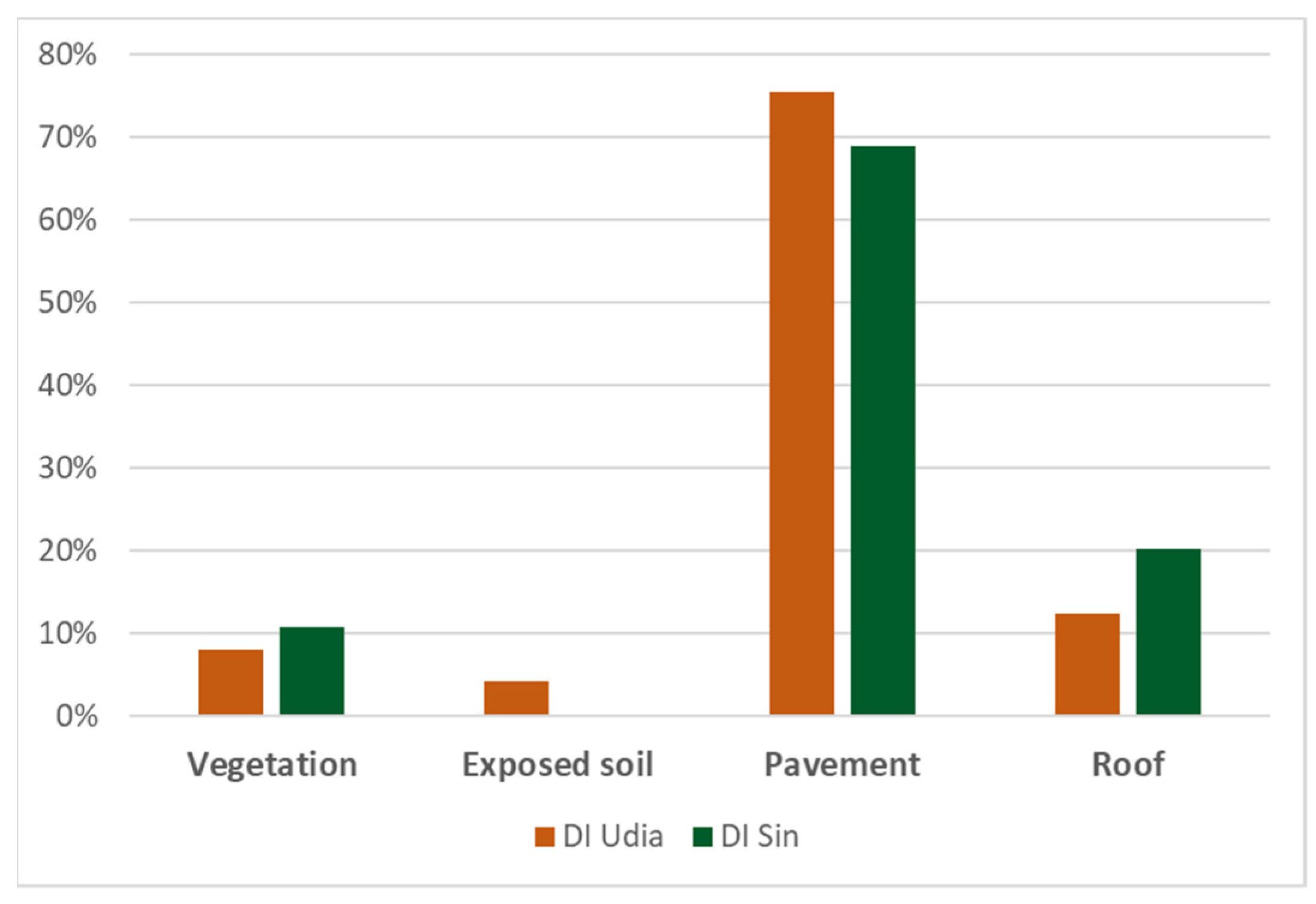
3.2. Physical Composition and Albedo of the Clippings
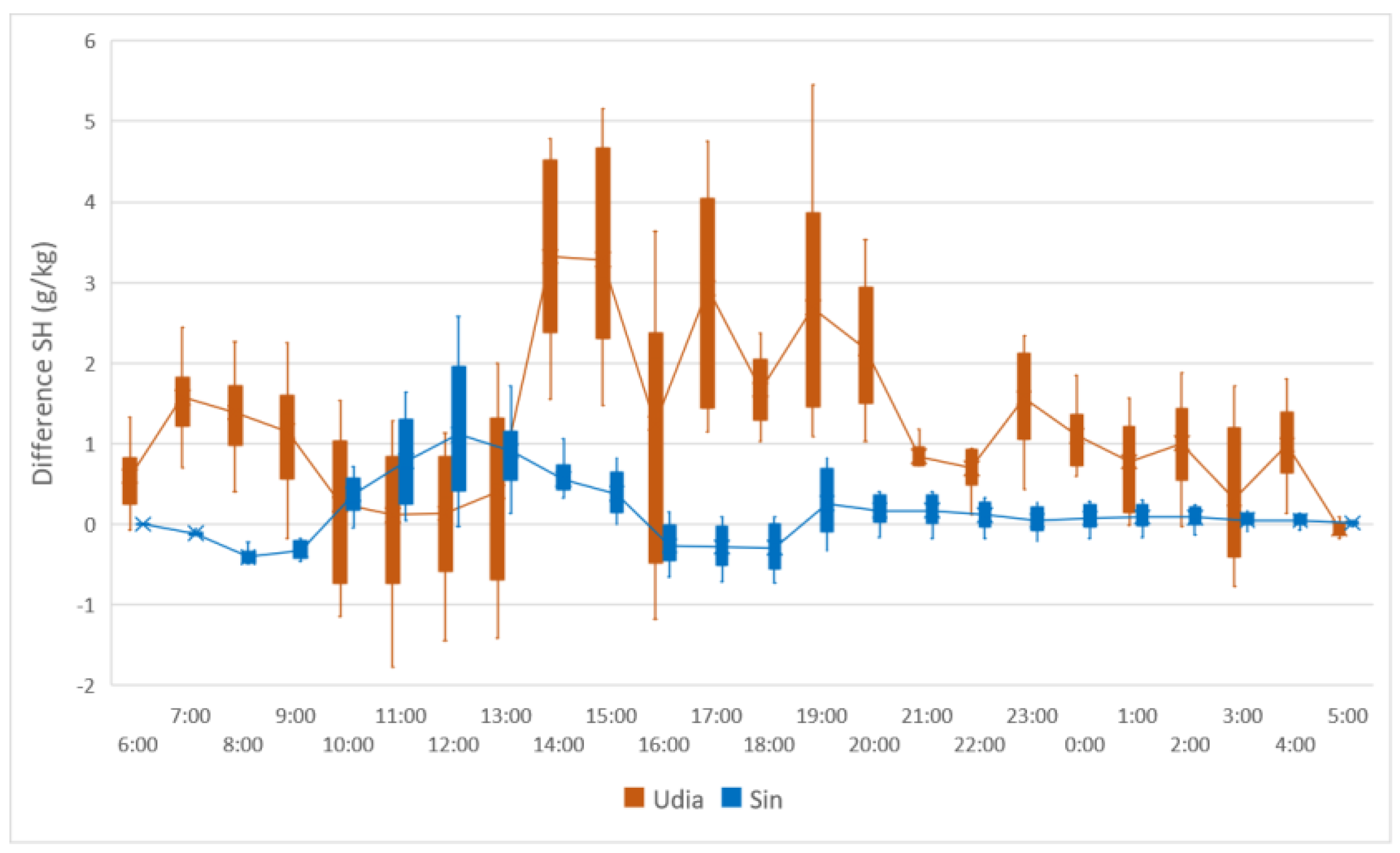
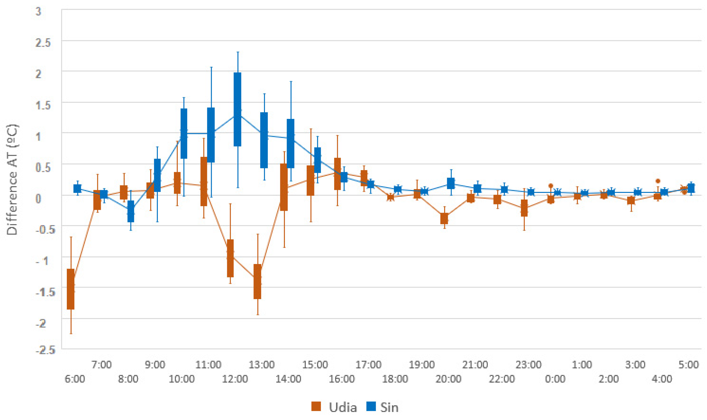
3.3. Descriptive Analysis
4. Discussion and Conclusions
Author Contributions
Funding
Conflicts of Interest
References
- Alcoforado, M.J. Fontes instrumentais e documentais para a reconstrução do clima do passado debatidas em conferência internacional. Finisterra 2012, 43, 157–159. [Google Scholar] [CrossRef]
- Oke, T.R. Boundary Layer Climates; Routledge: Oxfordshire, UK, 2002. [Google Scholar] [CrossRef]
- Huang, X.; Wang, Y. Investigating the Effects of 3D Urban Morphology on the Surface Urban Heat Island Effect in Urban Functional Zones by Using High-Resolution Remote Sensing Data: A Case Study of Wuhan, Central China. ISPRS J. Photogramm. Remote Sens. 2019, 152, 119–131. [Google Scholar] [CrossRef]
- Oke, T.R.; Johnson, G.T.; Steyn, D.G.; Watson, I.D. Simulation of Surface Urban Heat Islands under Ideal Conditions at Night Part 2: Diagnosis of Causation. Bound.-Layer Meteorol. 1991, 56, 339–358. [Google Scholar] [CrossRef]
- Amorim, M.C.D.C.T.; Dubreuil, V.; Cardoso, R.D.S. Modelagem Espacial Da Ilha de Calor Em Presidente Prudente/SP. Rev. Bras. Climatol. 2015, 16, 29–45. [Google Scholar] [CrossRef]
- Gartland, L. Ilhas de Calor: Como Mitigar Zonas de Calor em Áreas Urbanas, 1st ed.; Editora Oficina de Textos: São Paulo, Brazil, 2010. [Google Scholar]
- Romero, M.A.B.; Baptista, G.M.D.M.; de Lima, E.A.; Werneck, D.R.; Vianna, E.O.; Sales, G.D.L. Mudanças Climáticas e Ilhas de Calor Urbanas, 1st ed.; Universidade de Brasília: Brasília, Brazil, 2019. [Google Scholar]
- Bechtel, B.; Demuzere, M.; Mills, G.; Zhan, W.; Sismanidis, P.; Small, C.; Voogt, J. SUHI Analysis Using Local Climate Zones—A Comparison of 50 Cities. Urban Clim. 2019, 28, 100451. [Google Scholar] [CrossRef]
- Meng, Q.; Hu, D.; Zhang, Y.; Chen, X.; Zhang, L.; Wang, Z. Do Industrial Parks Generate Intra-Heat Island Effects in Cities? New Evidence, Quantitative Methods, and Contributing Factors from a Spatiotemporal Analysis of Top Steel Plants in China. Environ. Pollut. 2022, 292, 118383. [Google Scholar] [CrossRef]
- Stewart, I.D.; Oke, T.R. Local Climate Zones for Urban Temperature Studies. Bull. Am. Meteorol. Soc. 2012, 93, 1879–1900. [Google Scholar] [CrossRef]
- Stewart, I.D. Redefining the Urban Heat Island. Ph.D. Thesis, University of British Columbia, Vancouver, BC, Canada, 2011. [Google Scholar] [CrossRef]
- Mohan, M.; Singh, V.K.; Bhati, S.; Lodhi, N.; Sati, A.P.; Sahoo, N.R.; Dash, S.; Mishra, P.C.; Dey, S. Industrial Heat Island: A Case Study of Angul-Talcher Region in India. Theor. Appl. Climatol. 2020, 141, 229–246. [Google Scholar] [CrossRef]
- Xu, X.; Sun, S.; Liu, W.; García, E.H.; He, L.; Cai, Q.; Xu, S.; Wang, J.; Zhu, J. The Cooling and Energy Saving Effect of Landscape Design Parameters of Urban Park in Summer: A Case of Beijing, China. Energy Build. 2017, 149, 91–100. [Google Scholar] [CrossRef]
- Lu, M.; Zeng, L.; Li, Q.; Hang, J.; Hua, J.; Wang, X.; Wang, W. Quantifying cooling benefits of cool roofs and walls applied in building clusters by scaled outdoor experiments. Sustain. Cities Soc. 2023, 97, 104741. [Google Scholar] [CrossRef]
- Susca, T.; Zanghirella, F.; Del Fatto, V. Building integrated vegetation effect on micro-climate conditions for urban heat island adaptation. Lesson learned from Turin and Rome case studies. Energy Build. 2023, 295, 113233. [Google Scholar] [CrossRef]
- Peluso, P.; Persichetti, G.; Moretti, L. Effectiveness of Road Cool Pavements, Greenery, and Canopies to Reduce the Urban Heat Island Effects. Sustainability 2022, 14, 16027. [Google Scholar] [CrossRef]
- Yan, S.; Zhang, T.; Wu, Y.; Lv, C. Cooling Effect of Trees with Different Attributes and Layouts on the Surface Heat Island of Urban Street Canyons in Summer. Atmosphere 2023, 14, 857. [Google Scholar] [CrossRef]
- Mao, N. Analysis of Urban Street Microclimate Data Based on ENVI-Met. In Big Data Analytics for Cyber-Physical System in Smart City; Atiquzzaman, M., Yen, N., Xu, Z., Eds.; Advances in Intelligent Systems and Computing; Springer: Singapore, 2020; Volume 1117. [Google Scholar] [CrossRef]
- Flanner, M.G. Integrating Anthropogenic Heat Flux with Global Climate Models: Anthropogenic heat flux and climate. Geophys. Res. Lett. 2009, 36, 1–5. [Google Scholar] [CrossRef]
- Croce, S.; D’Agnolo, E.; Caini, M.; Paparella, R. The Use of Cool Pavements for the Regeneration of Industrial Districts. Sustainability 2021, 13, 6322. [Google Scholar] [CrossRef]
- Gao, J.; Meng, Q.; Zhang, L.; Hu, D. How Does the Ambient Environment Respond to the Industrial Heat Island Effects? An Innovative and Comprehensive Methodological Paradigm for Quantifying the Varied Cooling Effects of Different Landscapes. GIScience Remote Sens. 2022, 59, 1643–1659. [Google Scholar] [CrossRef]
- Singh, P.; Mahadevan, B.; Datta, A.; Sinha, V.S.P.; Pahuja, N. Heat Island Effect in an Industrial Cluster—Identification, Mitigation and Adaptation. Energy Resour. Inst. Teri. 2017, 1–11. [Google Scholar] [CrossRef]
- Reis, C.; Lopes, A.; Nouri, A.S. Assessing Urban Heat Island Effects through Local Weather Types in Lisbon’s Metropolitan Area Using Big Data from the Copernicus Service. Urban Clim. 2022, 43, 101168. [Google Scholar] [CrossRef]
- Reis, C.; Lopes, A.; Correia, E.; Fragoso, M. Local Weather Types by Thermal Periods: Deepening the Knowledge about Lisbon’s Urban Climate. Atmosphere 2020, 11, 840. [Google Scholar] [CrossRef]
- Noro, M.; Busato, F.; Lazzarin, R.M. Urban Heat Island in Padua, Italy: Experimental and Theoretical Analysis. Indoor Built Environ. 2015, 24, 514–533. [Google Scholar] [CrossRef]
- Silva, I.C.D.S. Índice Ambiental Urbano (IAU): Uma Contribuição ao Estudo do Planejamento e do Conforto Térmico em Espaços Abertos. Ph.D. Thesis, Federal University of Rio Grande do Norte, Natal, Brazil, 2017. [Google Scholar]
- Shinzato, P.; Duarte, D.H.S. Impacto Da Vegetação Nos Microclimas Urbanos e No Conforto Térmico Em Espaços Abertos Em Função Das Interações Solo-Vegetação-Atmosfera. Ambiente Construído 2018, 18, 197–215. [Google Scholar] [CrossRef]
- Rapti, T.; Kantzioura, A. Study of Urban Microclimate Conditions in a Commercial Area of an Urban Centre and the Environmental Regeneration Potential. IOP Conf. Ser. Earth Environ. Sci. 2021, 899, 012017. [Google Scholar] [CrossRef]
- Zhao, X.; He, J.; Luo, Y.; Li, Y. An Analytical Method to Determine Typical Residential District Models for Predicting the Urban Heat Island Effect in Residential Areas. Urban Clim. 2022, 41, 101007. [Google Scholar] [CrossRef]
- Ozkeresteci, I.; Crewe, K. Use and evaluation of the ENVI-met model for environmental design and planning: An experiment on linear parks. In Proceedings of the 21st International Cartographic Conference (ICC), Durban, South Africa, 10–16 August 2003; Cartographic Renaissance. pp. 402–409. [Google Scholar]
- Abrantes, P. Ordenamento e Planeamento Do Território. In AML—Área Metropolitana de Lisboa; Atlas Digital: Burbank, CA, USA, 2016. [Google Scholar]
- Portugal. Instituto Nacional de Estatística (INE). Available online: https://www.ine.pt/xportal/xmain?xpgid=ine_main&xpid=INE (accessed on 28 March 2023).
- Portugal. Instituto Português do Mar e da Atmosfera (IPMA). Available online: https://www.ipma.pt/pt/index.html (accessed on 28 March 2023).
- Brasil. Instituto Brasileiro de Geografia e Estatística (IBGE). Available online: www.ibge.gov.br (accessed on 26 April 2023).
- Demuzere, M.; Kittner, J.; Martilli, A.; Mills, G.; Moede, C.; Stewart, I.D.; van Vliet, J.; Bechtel, B. A Global Map of Local Climate Zones to Support Earth System Modelling and Urban-Scale Environmental Science. Earth Syst. Sci. Data 2022, 14, 3835–3873. [Google Scholar] [CrossRef]
- Climate.OneBuiding.Org. Available online: https://www.climate.onebuilding.org/ (accessed on 27 January 2023).
- Lopes, A.S.; Matias, M.; Oliveira, A.; Correia, E.; Reis, C. Identificação das Ilhas de Calor Urbano e Simulação para as áreas críticas da cidade de Lisboa. 2020. Available online: https://www.lisboa.pt/fileadmin/cidade_temas/ambiente/qualidade_ambiental/ondas_calor/Ondas_Calor/IdentificacaoICU_ATUAL_Fase1.pdf. (accessed on 25 March 2023).
- Masiero, É.; Christoforo, A.L.; Kowalski, L.F.; Fernandes, M.E. Urban Morphology and Prediction Models of Microclimatic Phenomena in Dry Atmospheric Context. Rev. Bras. Climatol. 2022, 31, 259–284. [Google Scholar] [CrossRef]
- Lopes, A. Cidades e Alterações Climáticas: Caderno de Trabalhos Práticos; Instituto de Ordenação Do Território (IGOT): Lisbon, Portugal, 2023. [Google Scholar]
- USA. USGS Earth Explorer. Available online: https://earthexplorer.usgs.gov/ (accessed on 27 January 2023).
- Olmedo, G.F.; Ortega Farias, S.; Fonseca Luengo, D.; Fuentes Peñailillo, F. Water: Tools and Functions to Estimate Actual Evapotranspiration Using Land Surface Energy Balance Models in R. R J. 2016, 8, 352. [Google Scholar] [CrossRef]
- Azevedo, A.M. MultivariateAnalysis para-R. Available online: https://cran.r-project.org/web/packages/MultivariateAnalysis/MultivariateAnalysis.pdf (accessed on 25 March 2023).
- Hongyu, K.; Sandanielo, V.L.M.; Junior, G.J. de O. Análise de Componentes Principais: Resumo Teórico, Aplicação e Interpretação. ES Eng. Sci. 2016, 5, 83–90. [Google Scholar] [CrossRef]
- Zscheischler, J.; Mahecha, M.D.; Harmeling, S. Climate Classifications: The Value of Unsupervised Clustering. Procedia Comput. Sci. 2012, 9, 897–906. [Google Scholar] [CrossRef]
- Amiri, M.A.; Mesgari, M. Modeling the Spatial and Temporal Variability of Precipitation in Northwest Iran. Atmosphere 2017, 8, 254. [Google Scholar] [CrossRef]
- Silva, C.M.A.d.; Barreto, Í.D.D.C.; Santos, E.A.B.d.; Santos, E.F.N.; Borges, P.D.F.; de Araújo, L.S. Análise Das Variáveis Climáticas Das Estações Agrometeorológicas Do Estado de Sergipe Através de Métodos Multivariados (2011–2013). Gaia Sci. 2017, 11, 144–156. [Google Scholar] [CrossRef]
- Leoni, R.C.; Sampaio, N.A.D.S.; Corrêa, S.M. Estatística Multivariada Aplicada Ao Estudo Da Qualidade Do Ar. Rev. Bras. Meteorol. 2017, 32, 235–241. [Google Scholar] [CrossRef]
- Santos, E.F.N.; Sousa, I.F. Análise Estatística Multivariada Da Precipitação Do Estado de Sergipe Através Dos Fatores e Agrupamentos. Rev. Bras. Climatol. 2018, 205–222. [Google Scholar] [CrossRef]
- Praene, J.P.; Malet-Damour, B.; Radanielina, M.H.; Fontaine, L.; Rivière, G. GIS-Based Approach to Identify Climatic Zoning: A Hierarchical Clustering on Principal Component Analysis. Build. Environ. 2019, 164, 1–29. [Google Scholar] [CrossRef]
- Valverde, M.C.; Coelho, L.H.; de Oliveira Cardoso, A.; Paiva Junior, H.; Brambila, R.; Boian, C.; Martinelli, P.C.; Valdambrini, N.M. Urban Climate Assessment in the ABC Paulista Region of São Paulo, Brazil. Sci. Total Environ. 2020, 735, 139303. [Google Scholar] [CrossRef]
- Kaiser, H.F. The Varimax Criterion for Analytic Rotation in Factor Analysis. Psychometrika 1958, 23, 187–200. [Google Scholar] [CrossRef]
- Gunawardena, K.R.; Wells, M.J.; Kershaw, T. Utilising Green and Bluespace to Mitigate Urban Heat Island Intensity. Sci. Total Environ. 2017, 584–585, 1040–1055. [Google Scholar] [CrossRef] [PubMed]
- Palomo Amores, T.R.; Sánchez Ramos, J.; Guerrero Delgado, M.; Castro Medina, D.; Cerezo-Narvaéz, A.; Álvarez Domínguez, S. Effect of Green Infrastructures Supported by Adaptative Solar Shading Systems on Livability in Open Spaces. Urban For. Urban Green. 2023, 82, 127886. [Google Scholar] [CrossRef]
- Mello, M.A.R.; Martins, N.; Sant’anna Neto, J.L. A Influência Dos Materiais Construtivos Na Produção Do Clima Urbano. Rev. Bras. Climatol. 2017, 5. [Google Scholar] [CrossRef]
- Ferreira, F.L. Medição Do Albedo e Análise Da Sua Influência Na Temperatura Superficial Dos Materiais Utilizados Em Coberturas de Edifícios No Brasil. Master’s Thesis, São Paulo University, São Paulo, Brazil, 2003. Available online: https://repositorio.usp.br/item/001319699 (accessed on 7 July 2023).
- Alchapar, N.L.; Pezzuto, C.C.; Correa, E.N.; Chebel Labaki, L. The Impact of Different Cooling Strategies on Urban Air Temperatures: The Cases of Campinas, Brazil and Mendoza, Argentina. Theor. Appl. Climatol. 2017, 130, 35–50. [Google Scholar] [CrossRef]
- Akbari, H.; Menon, S.; Rosenfeld, A. Global Cooling: Increasing World-Wide Urban Albedos to Offset CO2. Clim. Change 2009, 94, 275–286. [Google Scholar] [CrossRef]
- Murguia, C.; Valles, D.; Park, Y.; Kuravi, S. Effect of High Aged Albedo Cool Roofs on Commercial Buildings Energy Savings in U.S.A. Climates. Int. J. Renew. Energy Res. 2019, 9, 65–72. [Google Scholar] [CrossRef]
- Galusic, B. Ilhas de calor urbanas em São Carlos, SP e os impactos da permeabilidade dos revestimentos urbanos horizontais. Master’s Thesis, Urbanismo e Tecnologia, Universidade de São Paulo, São Carlos, Brazil, 2019. [Google Scholar] [CrossRef]
- Xu, H.; Lin, D.; Tang, F. The impact of impervious surface development on land surface temperature in a subtropical city: Xiamen, China: The impact of impervious surface development on land surface temperature. Int. J. Climatol. 2013, 33, 1873–1883. [Google Scholar] [CrossRef]
- Xiao, X.; Zhang, L.; Xiong, Y.; Jiang, J.; Xu, A. Influence of Spatial Characteristics of Green Spaces on Microclimate in Suzhou Industrial Park of China. Sci. Rep. 2022, 12, 9121. [Google Scholar] [CrossRef] [PubMed]
- Oliveira, A.; Lopes, A.; Correia, E.; Niza, S.; Soares, A. Heatwaves and Summer Urban Heat Islands: A Daily Cycle Approach to Unveil the Urban Thermal Signal Changes in Lisbon, Portugal. Atmosphere 2021, 12, 292. [Google Scholar] [CrossRef]
- Lopes, A. Lisbon Climate Modification Due to the Urban Growth Wind, Surface Heat Island and Energy Balance. Ph.D. Thesis, University of Lisbon, Lisbon, Portugal, 2003. Available online: http://zephyrus.ulisboa.pt/sites/default/files/pub/ts/phd_al_2003.pdf (accessed on 7 July 2023).
- Lopes, A.; Alves, E.; Alcoforado, M.J.; Machete, R. Lisbon Urban Heat Island Updated: New Highlights about the Relationships between Thermal Patterns and Wind Regimes. Adv. Meteorol. 2013, 2013, 487695. [Google Scholar] [CrossRef]
- Matias, M.; Lopes, A. Surface Radiation Balance of Urban Materials and Their Impact on Air Temperature of an Urban Canyon in Lisbon, Portugal. Appl. Sci. 2020, 10, 2193. [Google Scholar] [CrossRef]
- Zheng, Z.; Ren, G.; Gao, H.; Yang, Y. Urban ventilation planning and its associated benefits based on numerical experiments: A case study in beijing, China. Build. Environ. 2022, 222, 109383. [Google Scholar] [CrossRef]


| Category | Input | |
|---|---|---|
| Modeling area (L, W, H) (m) Grid cell (x, y, z) | 500 × 500 × 50 4 × 4 × 2 | |
| Cities | Uberlândia | Sintra |
| Configuration file | ||
| Simulation start date | 05:00 h (23 January 2022) | 05:00 h (17 July 2022) |
| Simulation end date | 04:59 h (24 January 2022) | 04:59 h (17 July 2022) |
| Simulation period | 24 h | 24 h |
| Meteorological input | AT max = 41 °C—17:00 h | AT max = 29 °C—12:00 h |
| AT min = 29 °C—06:00 h | AT min = 15 °C—05:00 h | |
| SH max = 12.5 g/kg—22:00 h | SH max = 13 g/kg—13:00 h | |
| SH min = 8 g/kg—13:00 h | SH min = 9 g/kg—21:00 h | |
| WS max = 3.6 m/s—11:00 h | WS max = 6 m/s—15:00 h | |
| WS min = 0—5:00 h | WS min = 0—7:00 h | |
| Material | Roof—sandwich roofing sheet | Roof—sandwich roofing sheet |
| Pavement—dark asphalt | Pavement—light asphalt | |
| Vegetation—grass and trees | Vegetation—grass and trees | |
| Eigenvalue | Variance Percent | Cumulative Variance Percent | |
|---|---|---|---|
| PC1 | 4.75 | 59.40 | 59.40 |
| PC2 | 1.40 | 17.62 | 77.02 |
| PC3 | 0.84 | 10.61 | 87.63 |
| PC4 | 0.70 | 8.75 | 96.39 |
| PC5 | 0.15 | 1.90 | 98.29 |
| PC6 | 0.09 | 1.14 | 99.43 |
| PC7 | 0.04 | 0.53 | 99.97 |
| PC7 | 0.002 | 0.028 | 100 |
| Variable | Weighting Coefficient | Correlation | ||
|---|---|---|---|---|
| PC1 | PC2 | PC1 | PC2 | |
| AT | −0.45 | −0.009 | −0.99 | 0.01 |
| RH | 0.44 | 0.12 | 0.97 | −0.15 |
| SH | −0.06 | 0.65 | −0.15 | −0.77 |
| WS | 0.42 | −0.12 | 0.93 | 0.14 |
| SVF | −0.11 | −0.58 | −0.25 | 0.70 |
| Albedo | 0.43 | 0.05 | 0.94 | −0.07 |
| WD | 0.10 | −0.45 | 0.23 | 0.53 |
| LST | −0.44 | 0.02 | −0.97 | −0.03 |
| Theoretical Albedo | Measured Albedo | |||
|---|---|---|---|---|
| Category | UI Sin | UI Udia | UI Sin | UI Udia |
| Vegetation | 0.27 * | 0.27 * | 0.28 | 0.21 |
| Roof | 0.57 ** | 0.57 ** | 0.50 | 0.26 |
| Pavement | 0.50 * | 0.20 * | 0.30 | 0.15 |
| Average | 0.44 | 0.34 | 0.36 | 0.20 |
| Standard Deviation | 0.12 | 0.16 | 0.09 | 0.04 |
Disclaimer/Publisher’s Note: The statements, opinions and data contained in all publications are solely those of the individual author(s) and contributor(s) and not of MDPI and/or the editor(s). MDPI and/or the editor(s) disclaim responsibility for any injury to people or property resulting from any ideas, methods, instructions or products referred to in the content. |
© 2023 by the authors. Licensee MDPI, Basel, Switzerland. This article is an open access article distributed under the terms and conditions of the Creative Commons Attribution (CC BY) license (https://creativecommons.org/licenses/by/4.0/).
Share and Cite
Arruda, A.M.d.; Lopes, A.; Masiero, É. Microclimate Multivariate Analysis of Two Industrial Areas. Atmosphere 2023, 14, 1321. https://doi.org/10.3390/atmos14081321
Arruda AMd, Lopes A, Masiero É. Microclimate Multivariate Analysis of Two Industrial Areas. Atmosphere. 2023; 14(8):1321. https://doi.org/10.3390/atmos14081321
Chicago/Turabian StyleArruda, Angela Maria de, António Lopes, and Érico Masiero. 2023. "Microclimate Multivariate Analysis of Two Industrial Areas" Atmosphere 14, no. 8: 1321. https://doi.org/10.3390/atmos14081321
APA StyleArruda, A. M. d., Lopes, A., & Masiero, É. (2023). Microclimate Multivariate Analysis of Two Industrial Areas. Atmosphere, 14(8), 1321. https://doi.org/10.3390/atmos14081321