Article

Ice Core 17O Reveals Past Changes in Surface Air Temperatures and Stratosphere to Troposphere Mass Exchange

by
Pradeep K. Aggarwal
1,*,†,
Frederick J. Longstaffe
2 and
Franklin W. Schwartz
3
1
International Atomic Energy Agency, 1400 Vienna, Austria
2
Department of Earth Sciences, The University of Western Ontario, London, ON N6A 3K7, Canada
3
School of Earth Sciences, The Ohio State University, Columbus, OH 43210, USA
*
Author to whom correspondence should be addressed.
Now retired from IAEA.
Atmosphere 2023, 14(8), 1268; https://doi.org/10.3390/atmos14081268
Submission received: 14 July 2023 / Revised: 4 August 2023 / Accepted: 7 August 2023 / Published: 10 August 2023
(This article belongs to the Section Meteorology)

Abstract

:
In this study, we have investigated the oxygen isotope compositions (δ17O and δ18O) of modern rain and ice cores using published isotopic data. We find that, contrary to existing interpretations, precipitation δ17O is influenced by two factors: mass-dependent fractionation (MDF), which occurs during ocean evaporation, and mass-independent fractionation (MIF), which happens in the stratosphere. The MDF contribution remains constant and can be understood by studying tropical rain, as the overall movement of mass in the tropics is upward toward the stratosphere. On the other hand, the MIF effect comes from the mixing of stratospheric air in the troposphere, which is a result of the Brewer–Dobson circulation. This MIF effect on precipitation 17O increases from the tropics toward the poles and is observed consistently in modern precipitation and ice cores. The relative δ17O and δ18O composition, denoted as ∆‘17O, in modern precipitation can be calibrated with surface air temperature, creating a new and independent tool for estimating past temperatures. We used this calibration along with the ∆‘17O of Antarctic and Greenland ice cores, and our reconstructed past temperatures are in excellent agreement with those derived from borehole thermometry or gas phase analysis of air trapped in the ice. The ∆‘17O method overcomes the problems associated with using δ18O alone for paleothermometry. Our findings align with climate models that suggest a weakening of the Brewer–Dobson circulation during the Last Glacial Maximum. Furthermore, our approach could be used to monitor future changes in stratosphere–troposphere mass exchange in response to a warming climate caused by increasing greenhouse gases.

1. Introduction

The oxygen and hydrogen isotope compositions (δ18O and δ2H) of polar ice offer strong evidence of both long-term and abrupt climate changes. Temporal and spatial variations in δ18O and δ2H facilitate reconstruction of recurrent climate changes in past glacial and interglacial cycles [1,2,3]. The use of isotopes to derive climatic information has focused on the quantification of surface air temperatures and changes in the hydrological cycle [4,5]. However, the δ18O–temperature relationship (δ/T slope) cannot be calibrated and yields different results when evaluated for spatial or temporal (e.g., ice cores at different depths) variations [6,7]. In coastal Antarctica, variations in the surface temperature do not appear to influence the δ18O of shallow ice cores [8]. The estimates of Greenland temperature changes from the Last Glacial Maximum (LGM, ~29–19 kyr before present) to the Holocene (~11.7 kyr to present), or during abrupt events, derived from ice core δ18O are much different than those derived from borehole thermometry [9,10] or gas phase analysis that uses models of firn densification and thermal fractionation of gases extracted from trapped air in the ice [11]. The δ18O-based estimates of temperature increase from the LGM to the Holocene are smaller by 10–16 °C compared to those based on borehole or gas phase analysis thermometry [9,11]. Similarly, the magnitude of cooling or warming during abrupt climate change events is smaller when estimated from δ18O than from trapped air in ice. Borehole thermometry is not applicable for quantifying abrupt temperature changes [6,7,9], and gas phase analysis of trapped air may be less reliable in regions of low snow accumulation such as East Antarctica [7]. Gas phase analysis can also yield conflicting temperature estimates because of differences in the models of heat and ice flow and firn densification. For example, at the NGRIP ice core site in Greenland, differing LGM temperatures or warming trends during deglaciation have been indicated based on the same dataset of gas phase compositions [12,13].
The hydrological cycle changes inferred from isotopic data have included the sea surface temperature and relative humidity in oceanic moisture source regions and the amount of precipitation or accumulation in polar areas [4,5]. Precipitation isotope variability is also weakly correlated with large-scale hemispherical modes (southern and northern annular modes) of circulation [4] that are connected to the stratosphere through changes in the strength of the polar vortices [14,15]. However, the precipitation δ18O and δ2H compositions are not useful for characterizing changes in stratosphere–troposphere interactions [16].
More recently, small but significant variations have been observed in the relative composition of precipitation δ17O versus δ18O. These differences have been interpreted to reflect a variable mass-dependent fractionation (MDF) owing to the variable relative humidity during ocean evaporation in the moisture source region [17,18,19,20]. The humidity-dependence of 17O, however, does not adequately explain the observed variations in polar precipitation and ice cores [21,22,23], leading to the suggestion that, in natural waters, MDF is associated with different coefficients from the tropics to the poles [24].
Commonly, interpretations of the 17O levels in natural waters do not account for the contributions from stratosphere-sourced 17O [17,18,19,20,21,22,24]. Mass-independent fractionation (MIF) during ozone photolysis reactions in the stratosphere produce much higher δ17O relative to δ18O compared to the δ17O ≈ 0.5 δ18O resulting from MDF [25]. A stratospheric input is known to influence the 17O contents of tropospheric gases (ozone, molecular oxygen and carbon dioxide) or nitrate and sulfate aerosols [25]. Stratospheric 17O influence has also been shown for Antarctic [26,27] and Arctic [28] snow, but it is not considered to be a ubiquitous source contributing normally to global precipitation [17,18,19,20,21,22,24].
Here, we investigate the roles of MDF and stratospheric input in determining the δ17O of precipitation by using the δ17O and δ18O values of tropical to polar precipitation and ice cores from the published literature. We then explore the relative difference between the δ17O and δ18O compositions (∆’17O) as an independent paleothermometer based on an empirical calibration with temperature data for modern precipitation. Our approach is based on the hypothesis that the ∆’17O is affected by stratospheric input when precipitation forms, but not by subsequent water cycle processes as those processes would all involve a mass-dependent fractionation that does not change the ∆’17O. Our results show that the ∆’17O of precipitation and ice cores provides a robust tool for monitoring stratosphere to troposphere mass exchange. The ∆’17O paleothermometer is robust and overcomes the limitations of using δ18O alone. It also inherently compensates for the effects of seasonality or the altitude of precipitation and different seawater δ18O compositions in the past.

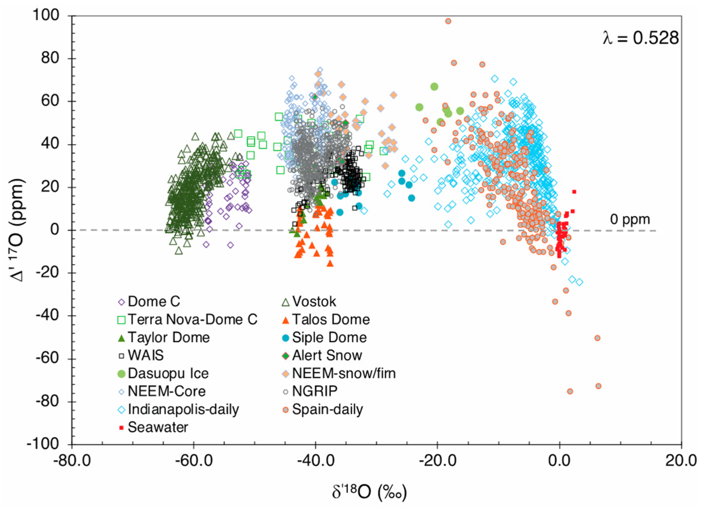
2. Stratospheric Input and Precipitation 17O

2.1. Mass-Dependent Fractionation Coefficient

Detailed descriptions and reviews of current knowledge concerning the 17O distribution in natural waters are available in the published literature [17,18,19,20,21,22,24,25,29]. Briefly, the kinetic or equilibrium MDF of oxygen isotopes in water cycle processes, such as evaporation, diffusion, and condensation, is expressed using the conventional δ notation as follows:
ln (1 + δ17O/1000) = λ ln (1+ δ18O/1000)
where δ = 103 (Rsample/Rstandard − 1), R is the isotope ratio (17O/16O or 18O/16O) in a sample or the VSMOW isotopic standard, and λ is a constant for mass-dependent fractionation (MDF coefficient). In the commonly used notation for triple isotope systems, Equation (1) is written as:
δ’17O = λ·δ’18O
The δ’ values are slightly more negative than the δ values and are preferred as the resulting δ’17O–δ’18O relationship becomes linear [22] Deviations from mass-dependent fractionation are given as [22]:
∆’17O (per meg or ppm) = 103 (δ’17O − λ δ’18O)
The MDF coefficient (λ) has a value of approximately 0.5 [22]. For natural waters, the actual fractionation processes are not easily quantified and therefore the λ value is determined empirically (Equation (2)) as the regression slope of δ’17O versus δ’18O [22]. This regression is conducted using a diverse set of natural water samples, and it is assumed that the 17O of those samples is affected only by mass-dependent isotope fractionation. A λ value of 0.528 has been determined [18,30] by using isotopic data of precipitation, lake, river, spring, and ice core samples from the tropics to Antarctica. The MDF coefficient of 0.528 yields ∆’17O values that are quite variable (Figure 1) for seawater, precipitation and ice cores [18,19,28,31,32,33,34,35,36,37,38,39,40]. These ∆’17O values have a positive or negative slope in the ∆’17O−δ’18O space, and are mostly greater than zero (Figure 1). A smaller proportion of water samples from all regions also has ∆’17O values that are less than zero (Figure 1).
Mass-dependent fractionation processes, by definition, result in ∆’17O values of zero [25]. Therefore, the positive or negative ∆’17O values in natural waters have been attributed to different MDFs in equilibrium (MDF λ ≈ 0.529) and kinetic (MDF λ ≈ 0.519) fractionation processes [17,18,41]. The proportions of equilibrium or kinetic fractionation processes are considered to vary depending upon the relative humidity during ocean evaporation in the moisture source region [17,18,19,20,21,22,24]. This ∆’17O behavior is analogous to that of the relative δ18O and δ2H composition (d-excess), which is also interpreted to reflect humidity and/or sea surface temperature variations in the moisture source region. However, the ∆’17O and d-excess in ice cores are not well correlated [21,22]. The ocean relative humidity during the LGM based on the ∆’17O of ice cores is inferred to be higher compared to present-day values. This finding appears to be inconsistent with recent observational trends or climate model predictions [23]. Following several studies with extensive isotopic datasets, the humidity dependence of MDF in the moisture source region has been insufficient to explain the observed ∆’17O variations in precipitation and ice cores [21,22].
An alternative is that the MDF coefficient in water cycle processes may simply be variable in polar and non-polar precipitation instead of a constant value of 0.528 [24]. There is, however, no mechanism available for quantifying the geographical or climatic variations in the MDF coefficient. Consequently, the causes of the ∆’17O variability in modern or past precipitation remain poorly understood [21,22,23].
It is also possible that all sources and processes affecting natural water 17O levels are not included in the presently accepted MDF coefficient of 0.528. As noted above, this coefficient was estimated from a dataset that included samples of Antarctic ice [18,19,30], which has been shown to contain a stratospheric input [26,27]. Similarly, upper tropospheric moisture contributing to extratropical precipitation may also include a MIF component because of the stratosphere to troposphere transport that occurs mostly at high latitudes [42]. Indeed, a lower MDF coefficient of 0.525 is obtained when Antarctic and mid- to high-latitude samples are excluded from the presently used reference dataset of Luz and Barkan [18]. That coefficient is lowered further to 0.523 when lakes and ponds also are excluded, as the δ17O in some of these samples is considered to have been affected by evaporation [18]. Therefore, the existing evidence indicates that the influence of the stratospheric input of 17O must be evaluated in order to characterize the MDF coefficient for natural waters.
Stratospheric air, including water vapor, reaches the troposphere via stratosphere to troposphere transport (STT) driven by the meridional Brewer–Dobson circulation (BDC) [42,43]. The BDC acts as an “extratropical pump” (Figure S1), with an upwelling of tropospheric air across the tropopause in the tropics (23° N–23° S latitude), poleward transport within the stratosphere, and a downwelling of stratospheric air at high latitudes (poleward of ~60° N or ~50° S) of the winter hemisphere [42,43]. Tropospheric moisture in the tropics is derived mostly from ocean evaporation (Figures S1 and S2), and the water vapor mixing ratio decreases with altitude to ~10 ppmv near the tropopause (~10–18 km) [23,42]. This air is further dehydrated to a mixing ratio of ~2–3 ppmv via freeze-drying across the tropopause before entering the stratosphere [42].
The δ17O of the tropospheric air entering the stratosphere reflects mass-dependent fractionation (δ17O ≈ 0.5 δ18O) in ocean evaporation [44,45]. In the stratosphere, water vapor δ17O increases through isotope exchange with NOx species, which have a higher 17O abundance owing to MIF in ozone photolysis reactions [25,44,45,46]. The water vapor mixing ratio of stratospheric air nearly doubles to ~4–6 ppmv [42] by in situ production of water via methane oxidation. This water also has higher δ17O because oxygen in methane oxidation carries an MIF imprint [44,45,46].
Stratospheric water vapor with elevated δ17O reaches the troposphere in the downward flow of the BDC at high latitudes. Higher δ17O/δ18O ratios (with ∆’17O values of ~−2000 ppm) have been observed in upper tropospheric moisture just below the tropopause poleward of ~64° S latitude [44]. As the net vertical transport of water vapor in the tropics is toward the stratosphere [42,43], the latitudinal variability in STT would also result in variable δ17O/δ18O ratios (or ∆’17O) of the upper tropospheric moisture.
Upper tropospheric moisture is in turn incorporated in precipitation [47,48]. This is indicated by the ubiquitous presence of cosmogenic tritium in precipitation because tritium is produced predominantly in the stratosphere and is also carried to the troposphere via STT [49,50]. Latitudinal variability in the δ17O/δ18O ratios (or ∆’17O) of upper tropospheric moisture therefore can be reflected in precipitation. An inverse correlation of tritium and δ18O is observed in Antarctic surface snow (Figure S3). This suggests that a tropospheric moisture component influenced by STT may contribute to the lower δ18O of Antarctic precipitation [26]. In non-polar regions, stratiform-type precipitation, which originates largely from tropospheric moisture [47,48], has lower δ18O compared to convective-type precipitation [51], which originates mostly from moisture in the planetary boundary layer [47,48]. Consequently, the δ17O of precipitation may also include a variable component of stratospheric input.
Once precipitation is formed, however, subsequent fractionation in water cycle processes (for example, evaporation, sublimation, diffusion, or isotopic exchange in surface snow) would all be mass-dependent with δ17O ≈ 0.5 δ18O [44]. In other words, if precipitation at different latitudes or in different seasons forms with a tropospheric moisture component that has variable δ17O/δ18O ratios, this variability in the isotopic ratios (or ∆’17O) would be preserved because any subsequent isotopic fractionation would be mass-dependent and change the δ17O value by approximately half that of the δ18O. Indeed, high latitude precipitation poleward of 60° N or 60° S has a δ’17O versus δ’18O regression slope of 0.529, compared to a slope of 0.527 at lower latitudes toward the equator [24,29].
The stratospheric 17O inputs are minimal in the tropics, where the net vertical mass flux is toward the stratosphere. At mid- to high-latitudes, the stratospheric inputs increase owing to the Brewer–Dobson circulation (Figure S1; Refs. [42,43,44]). Therefore, we can characterize the coefficient of mass-dependent fractionation by evaluating the δ’17O−δ’18O relationships in tropical and extratropical precipitation. This approach is similar to that used for identifying a stratospheric component in tropospheric O2 [52].
We compile the δ’17O and δ’18O values of 858 samples of precipitation and surface water from the published literature [18,28,53,54,55,56,57,58,59]. These data are separated into subsets of tropical (about 23° N–23° S latitude), sub-tropical (about 23° to 30° N or S) and extratropical (30° to 60° N or S) regions.
The δ’17O versus δ’18O regression slope for tropical precipitation and surface waters (elevation < 1000 m) is 0.521 (Table 1). The combined regression of tropical and subtropical waters also has a slope of 0.521. That value increases to 0.523 when high elevation (~1000 to ~4600 m) tropical waters (with low δ18O values) are included in the regression. Conversely, tropical and subtropical waters with higher δ’18O values (>−4‰) have a lower slope of 0.516 (n = 133). Although the stratospheric input in the tropics is minimal, some of the deep convective and other precipitation may still be influenced by it. Combined isotope and radar studies of precipitation events in California, USA have suggested that lower δ18O precipitation originates at higher altitudes [60]. As noted previously, the δ18O of precipitation has been shown to decrease with an increasing proportion of stratiform-type precipitation [51] that originates mostly from tropospheric moisture [47,48]. Nearly half of the precipitation in the tropics consists of the stratiform fraction [48]. The lower regression slope of 0.516 for the higher δ18O samples suggests that tropical water samples with lower δ18O may carry some influence of stratospheric 17O.
Regression of data from extratropical precipitation alone or together with tropical and subtropical waters gives higher slopes of 0.525 to 0.527 (Table 1). These higher slopes are consistent with a greater influence of stratospheric input in extratropical regions compared to the tropics. Regression of the subset of extratropical precipitation samples with δ’18O > −4‰ again results in a lower slope (~0.520) compared to that (0.529) for samples with δ’18O < −4‰. A combined regression of all higher δ’18O (> −4‰) samples in our dataset, including those from the extratropics, results in a regression slope of 0.516, as was noted above for samples only from the tropics (Table 1).
The regression intercepts are statistically significant (p-values < 0.01) for extratropical precipitation or subsets that include low δ’18O (< −4‰) extratropical precipitation. For all other subsets of tropical, subtropical and high δ’18O (> −4‰) extratropical precipitation, the intercepts are statistically insignificant, with p-values of 0.13 to 0.93 (Table 1). Thus, the δ’17O versus δ’18O regression line for tropical precipitation passes through the origin and indicates that water vapor from ocean evaporation does not have an anomalous 17O compared to that expected from MDF, contrary to the conclusions of previous studies [18,19].
The 0.516 value for the regression slope of heavier δ’18O waters (>−4‰) is nearly the same as the MDF coefficients in other terrestrial processes, including diffusion in air [41], plant photosynthesis [61], and leaf water evaporation [62]. It is likely therefore that for natural waters also the MDF coefficient has a value of ~0.516. This value is not substantially different than the 0.521 value obtained from the regression of tropical precipitation alone, excluding high elevations samples (Table 1). In the discussion below, we use 0.516 as the MDF coefficient to evaluate the stratospheric input and MDF influence on natural waters. This discussion remains essentially the same if a value of 0.521 is used, and we have included the corresponding figures in the Supporting Information.

2.2. Influence of Stratospheric Input on ∆’17O

The influence of the stratospheric 17O input on precipitation ∆’17O can be evaluated by examining its variability in ice cores, seawater and extratropical precipitation with respect to mass-dependent fractionation in tropical precipitation. As Figure 1 shows, the MDF coefficient value of 0.528 yields variable ∆’17O−δ’18O correlations for polar snow and ice cores, tropical glaciers, seawater and extratropical precipitation. The same data, however, show a strong correlation with a coefficient value of 0.516 (Figure 2) or 0.521 (Figure S4). The distribution of all of the Antarctic and Arctic snow or ice core samples is defined by a single regression line (R2 = 0.996). Extratropical precipitation with δ’18O < −4‰ and ice cores from tropical glaciers (Dasuopu) also lie along this trend (Figure 2A). We note that extratropical precipitation with unusually low δ’18O (~−31 to −28‰) has nearly the same ∆’17O as Greenland surface snow in a comparable δ’18O range (Figure 2A). Low δ18O in extratropical precipitation commonly occurs during extreme weather conditions, with a polar vortex and subsidence of drier, upper tropospheric air [63], which would cause the ∆’17O values to be similar to polar precipitation.
Seawater and extratropical precipitation with δ’18O greater than about −4‰ do not follow the ∆’17O−δ’18O correlation trend defined by polar snow and ice (Figure 2A). The ∆’17O of these samples is nearly zero, consistent with only mass-dependent fractionation affecting their 17O content. This lack of ∆’17O−δ’18O correlation in seawater and higher δ’18O precipitation remains the same with an MDF coefficient of 0.521 (Figure S4). Asthe coefficient values of 0.521 is derived from a regression of all the data, including δ’18O > −4‰, the selection of data used for estimating the MDF coefficient of 0.516 does not influence the lack of ∆’17O−δ’18O correlation in seawater and higher δ’18O precipitation.
The ∆’17O magnitude of Antarctic surface snow from near the Terra Nova coast to Dome C (Figure 2B) increases nearly twofold (albeit as negative values), as does its tritium content (Refs. [64,65]; Figure S3). This observation supports the correlation of increasing ∆’17O magnitude with greater stratospheric input, because tritium is a proxy for stratosphere to troposphere mass transport [26,49,50].
The increasingly negative values of ∆’17O attributed to an increasing stratospheric input may appear to be counter-intuitive because the stratospheric input has higher 17O levels than tropospheric moisture. However, this is an artifact of the definition of ∆’17O—it is defined relative to δ’18O—and the very low δ’18O of stratospheric input. We can evaluate the impact of the stratospheric 17O input on the numerical values of ∆’17O by using a two-component mixing model. Let f be the fraction of the stratospheric moisture component and r be the δ’17O/δ’18O ratio in the stratospheric (st) or tropospheric (tr) fractions. Because tropospheric moisture would only have mass-dependent fractionation, rtr is equivalent to λ, the MDF coefficient. Then,
δ’18Omix = f δ’18Ost + (1−f) δ’18Otr = f δ’18Ost + δ’18Otrf δ’18Otr
δ’17Omix = f δ’17Ost + (1−f) δ’17Otr = f rst δ’18Ost + λ δ’18Otrf λ δ’18Otr
and
∆’17Omix = 1000 (δ’17Omix − λ δ’18Omix)
Substituting (4) and (5) in (6) yields:
∆’17Omix = 1000 (f (rst − λ) δ’18Ost)
Because the value of δ’18Ost would always be a negative number [16], Equation (7) shows that an increasing stratospheric fraction would result in ∆’17O values that may be increasingly negative or positive depending upon rst being greater than or less than λ. An approximate value of rst can be obtained from winter Antarctic precipitation when the stratospheric input into the troposphere occurs via the Brewer–Dobson circulation [42,43] and upper tropospheric air descends to low elevations near the ground surface [66]. Regression of δ’17O versus δ’18O in winter Antarctic precipitation and surface snow [31,37] gives an rst value of 0.530.
Thus, with a λ value that is less than the estimated rst (e.g., 0.516 or 0.521), the ∆’17O values would be negative and become more negative with an increasing stratospheric fraction. For λ values greater than rst (e.g., 0.534), the ∆’17O values would be positive. We observe the same patterns of ∆’17O−δ’18O correlations in tropical to polar precipitation (Figure 2 and Figure S4). If the λ value were to be closer to the rst, and may be higher or lower than the rst at different latitudes, the ∆’17O values would be both positive or negative and decrease or increase with decreasing δ’18O. Such variable ∆’17O−δ’18O relationships are observed in tropical to polar precipitation with λ = 0.528 (Figure 1).

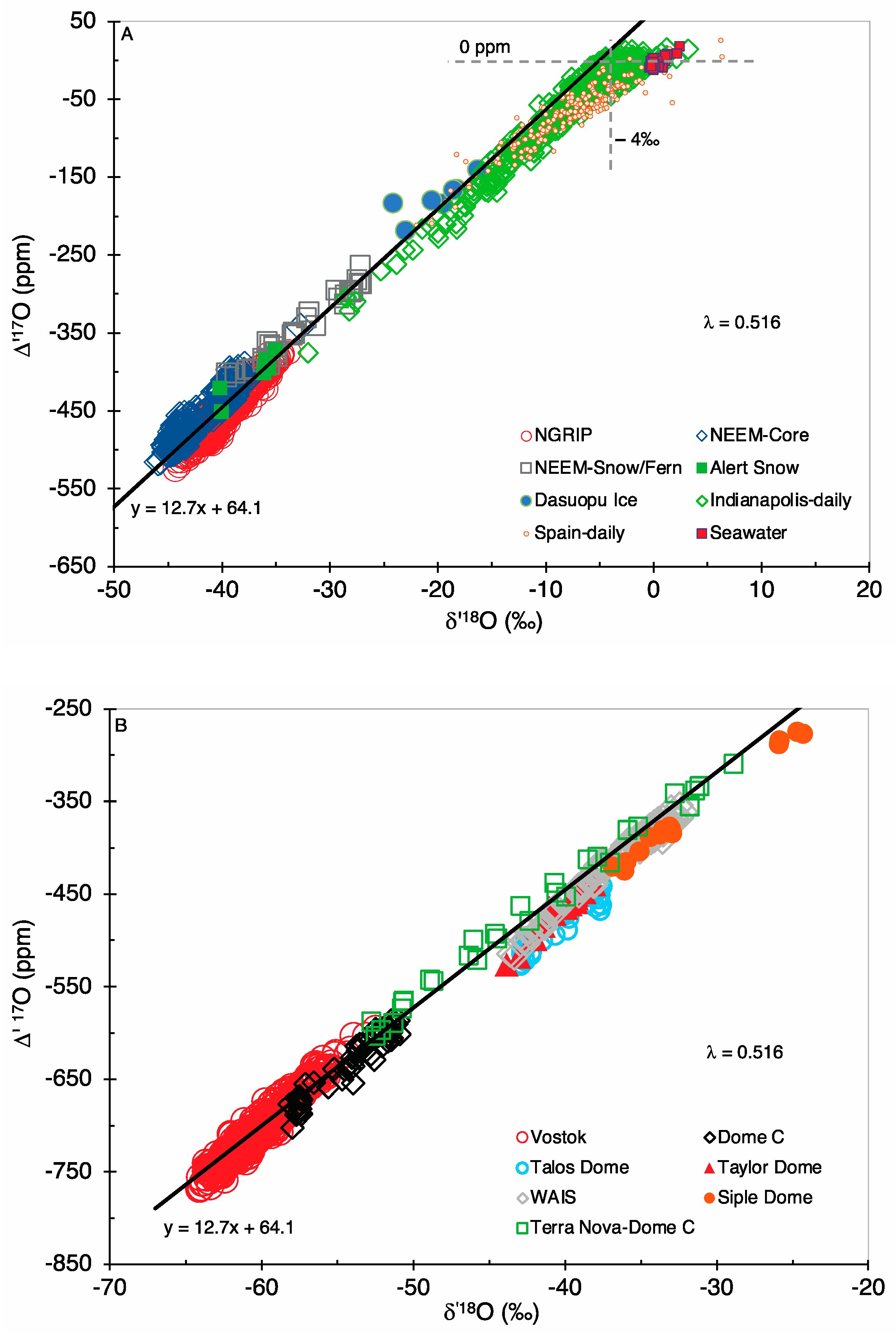
3. The ∆’17O Paleothermometer
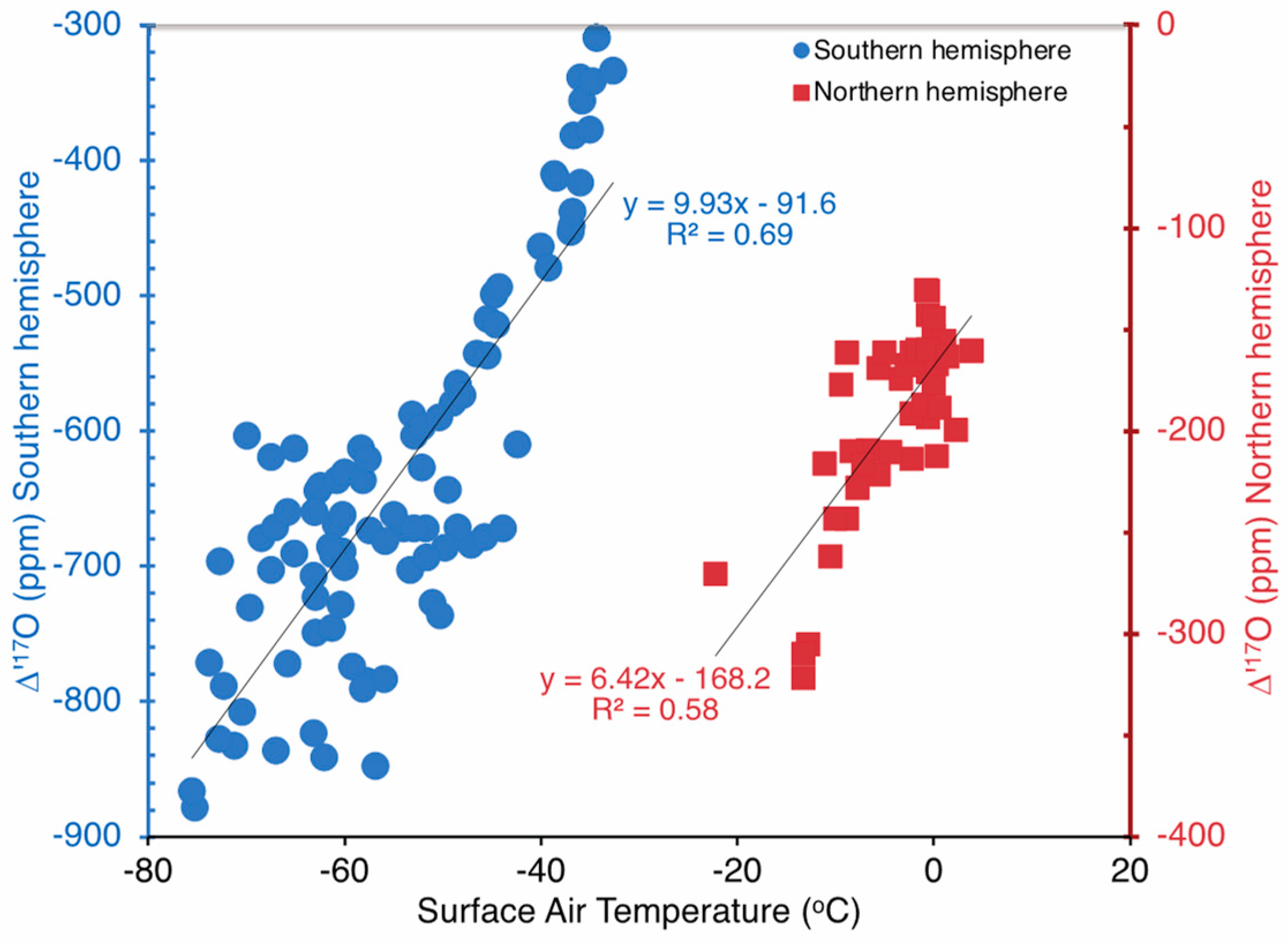
The greater magnitudes of ∆’17O in polar ice cores and the common correlation of ∆’17O with δ’18O in polar and extratropical precipitation (Figure 2) support our hypothesis that the ∆’17O variations resulting from the stratospheric 17O input to the troposphere are conserved in precipitation. Thus, the ∆’17O of precipitation may essentially be “fixed” once precipitation forms in the cloud. Any subsequent changes in precipitation δ17O and δ18O (by evaporation, diffusion, etc.) would occur via mass-dependent fractionation that would change the individual isotopic abundances but not the ∆’17O, because the ∆’17O of mass-dependent fractionation is zero [25]. In other words, the behavior of ∆’17O would be similar to that of a conservative tracer that is imparted to precipitation during its formation in the cloud, with the tracer concentration governed by the condensation temperature, and subsequently, remaining unchanged in the water cycle. Thus, instead of δ18O, ∆’17O may provide a more robust and independent basis for reconstructing surface temperatures from ice core data. A ∆’17O paleothermometer implies that the condensation temperatures are correlated with the surface air temperature, an assumption that is commonly used in isotope paleothermometry [3,67].

3.1. Calibration

We calibrated the ∆’17O paleothermometer empirically via the regression of the ∆’17O of modern precipitation versus its surface air temperature. Separate calibration data were used for Antarctica and Greenland because of the hemispherical asymmetry in the stratospheric input [43]. Ideally, a reasonably large database of ∆’17O in precipitation would be helpful for this calibration. However, we only had a relatively small dataset where both temperature and isotopic data are available. For Antarctica, precipitation data from Vostok and Dome C were supplemented with data for the surface snow from the Terra Nova coast to Dome C [31,37,38]. This de facto combination of temporal and spatial isotope variations is compatible with our hypothesis for the ∆’17O variations. Data for summer months (November–February) were excluded so that the precipitation would contain the maximum stratospheric input and minimal mixing with lower tropospheric moisture [15]. We did not find isotopic data for Greenland precipitation where temperature measurements also were reported. Therefore, we developed a calibration for the Northern hemisphere by using extratropical precipitation data from the south–central USA (Indianapolis; ref. [39]) and Europe (Madrid, Spain; ref. [40]) that partly overlap with the Greenland surface snow (Figure 2A). Only winter precipitation (December, January, February) data were used that were filtered to a δ18O value less than −15‰. These low δ18O samples lie on or closest to the ∆’17O − δ’18O regression line for polar ice and snow (Figure 2) and would consist mostly of stratiform precipitation [51]. The temperature measurements for the south–central USA precipitation were reported from a nearby weather station and have a greater uncertainty. A statistical analysis of the extratropical precipitation data identified two samples as outliers. These samples have been excluded from the calibration dataset.
The ∆’17O and temperature data are well correlated (R2 = 0.69 or 0.58), both for the Southern and Northern hemispheres (Figure 3), even though the calibration data are relatively small in number (n = 93 and 42, respectively). These correlations remain the same for an MDF coefficient of 0.521 (Figure S5). The equations for the ∆’17O paleothermometer (λ = 0.516) are:
  • Southern Hemisphere (Antarctic): ∆’17O = 9.93 T (°C) − 91.6
  • Northern Hemisphere (Greenland): ∆’17O = 6.42 T (°C) − 168.2
A regression of the estimated and measured temperatures for the two calibration datasets shows a strong correlation (Test. = 1.001 Tmeas. − 0.097; R2 = 0.92). The standard error of this regression suggests an uncertainty of ±7 °C for the ∆’17O paleothermometer. This apparently large uncertainty reflects the small amount of data available for calibration. The actual uncertainty likely is much smaller, as indicated by the similar magnitudes of the temperature changes in different climates between our reconstruction and previous studies (Figure 4). The uncertainty from the reported analytical error in the ∆’17O (±10 ppm) is much smaller (±1.5 °C) and subsumed within the larger statistical uncertainty.

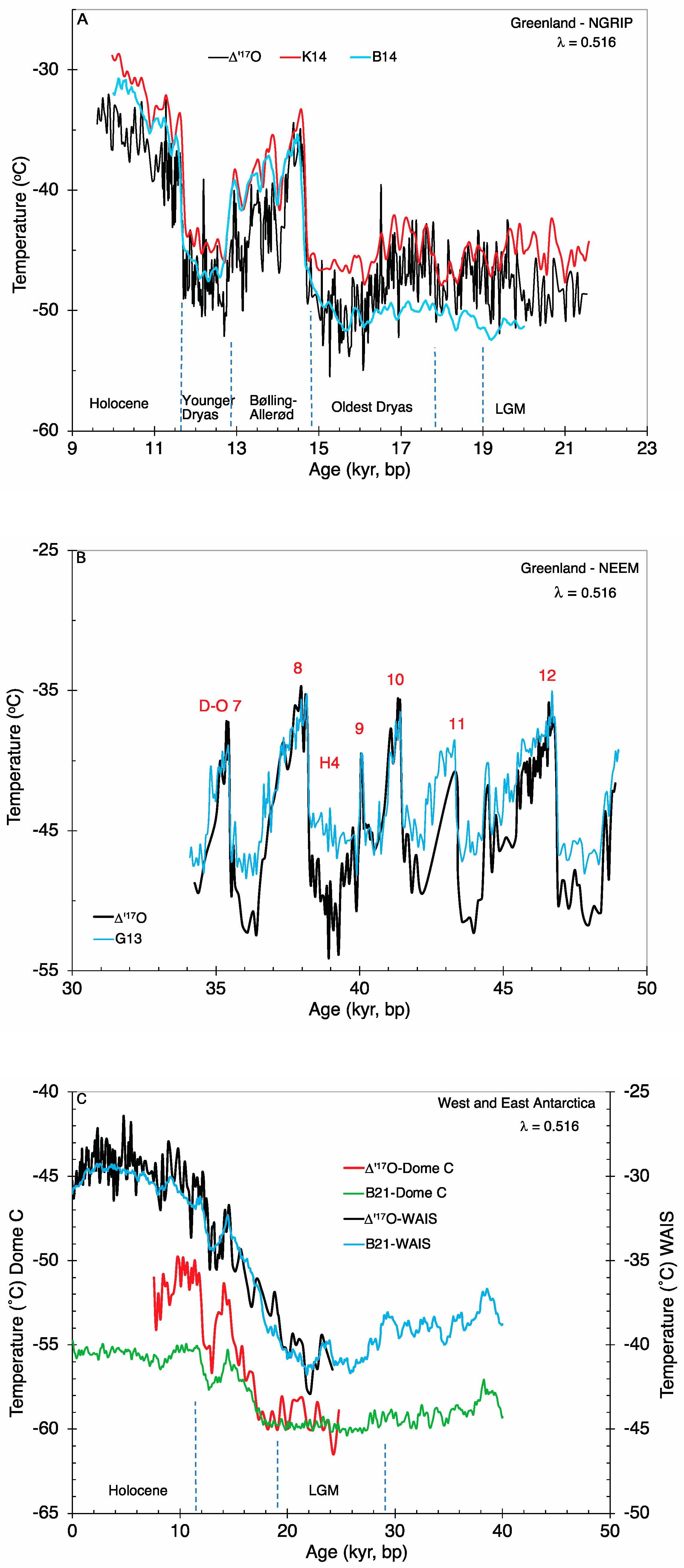
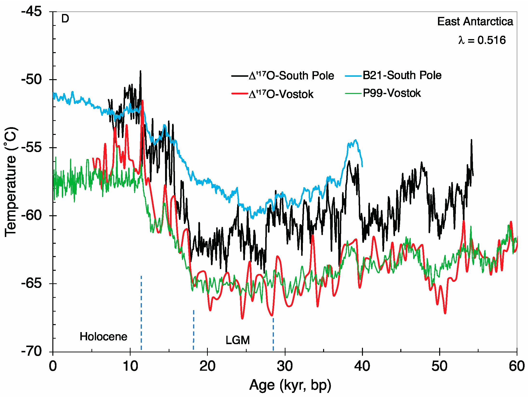
3.2. Temperature Reconstruction

The reconstructed surface air temperatures using the ∆’17O of ice cores from Greenland (NGRIP and NEEM), West Antarctica (WAIS) and East Antarctica (Dome C, South Pole, Vostok) are shown in Figure 4. The use of ∆’17O overcomes the deficiencies in isotope paleothermometry based on δ18O [9,10,12]. Specifically, the LGM to the Holocene temperature rise in Greenland based on ∆’17O is about 16 °C (Figure 4A), nearly twice that based on δ18O but similar to that derived via borehole thermometry [9].
Similarly, our estimated temperature changes during abrupt climate change events (warming in the Bølling–Allerød interstadial, cooling in the Younger Dryas, or Dansgaard–Oeshger events 7 to 12) are ~10 °C to 16 °C (Figure 4A,B). These ∆’17O based estimates are much higher than those estimated by using δ18O data, but are in excellent agreement with those estimated from gas phase analysis of air trapped in the ice [11,13,68]. With an MDF coefficient of 0.521, the estimated temperatures (Figure S6) are slightly warmer than those based on a coefficient value of 0.516 (Figure 4), but the magnitudes of temperature change from the LGM to the Holocene, or during abrupt events, remain the same.
For the NGRIP ice core (Figure 4A), the same gas composition data but different firn densification models provide conflicting temperature estimates, particularly for ages older than about 15 kyr [12,13] (hereafter B14 and K14, respectively). A significant warming trend earlier than the onset of the Bølling–Allerød interstadial at 14.7 kyr is identified in B14 but not in K14, and the estimated LGM temperatures at ~20 kyr are slightly colder (~−51 °C) in B14 than in K14 (~−46 °C). Our results show a warming trend beginning at ~15.7 kyr, in agreement with B14, although our LGM temperatures of ~−46 °C agree more with K14 and with those estimated via borehole thermometry [9].
The temperatures determined using ice core ∆’17O from NEEM (Figure 4B) also are in excellent agreement with those estimated in a previous study using gas phase analysis [68]. The original NEEM reconstruction of Guillevic et al. [68] was nearly the same as that for NGRIP, although the latter estimates have since been revised using different firn densification models [13]. This revision led to the NGRIP temperatures being warmer by ~4 °C. Therefore, we scaled the NEEM estimates accordingly in Figure 4B. We can also estimate the present-day surface air temperature at NEEM using the ∆’17O of shallow core samples of firn/snow for the years 2003–2005 [33]. Our estimated temperature of about −26 °C compares with an estimate of –26.5 °C reconstructed using gas phase analysis [69].
With data from Antarctic ice cores, our temperature reconstructions using the ∆’17O paleothermometer (Figure 4C,D) indicate an ~10–11 °C cooling during the LGM compared to the Holocene, both in the West (WAIS) and in the East (Dome C, South Pole, Vostok). Our results for West Antarctica (WAIS, Figure 4C) are in excellent agreement with those obtained using borehole thermometry [10] or by using both borehole and gas phase analysis [67] (hereafter B21). However, for East Antarctica, B21 suggests that the LGM cooling may have been only half (~4–7 °C) of that in the West. This is inconsistent with our results, which indicate similar degrees of cooling in West and East Antarctic. This discrepancy arises from the East Antarctic reconstructions where B21 estimated a much earlier initiation of warming at the South Pole (beginning at ~25 kyr), and relatively colder Holocene temperatures at Dome C, compared to our estimates (Figure 4C). The earlier initiation of the South Pole warming trend is unlikely as it would initiate deglaciation within the LGM and is inconsistent with their own results for Dome C ice core (Figure 4C). The discrepancy between our results and B21 may also arise from a greater uncertainty in our limited dataset for calibration. However, we note that the slopes and intercepts for the regression of the Antarctic snow and extratropical precipitation datasets (Figure 3 and Figure S5) are similar despite the hemispherical differences in the stratospheric input. This similarity suggests that larger datasets may result in only minor revisions to the calibration used in this study. Alternatively, the discrepancy between our results and B21 may reflect a greater uncertainty in models of heat and gas diffusion and firn densification in regions of low snow accumulation [7], given that our results are in excellent agreement with those of B21 for the high accumulation WAIS core site in West Antarctica (Figure 4C). Our results for the Vostok ice core in the low snow accumulation East Antarctic agree broadly with those based on spatial variations in δ2H [3]. However, the magnitude of the temperature changes from the LGM to the Holocene or other longer-term climate changes are lower in the δ2H-based reconstructions (as is the case for the Greenland estimates based on δ18O) compared to our results. A temperature reconstruction based on gas phase analysis was not available for the Vostok ice core.

4. Discussion

The magnitude of the temperature changes (and of the ∆’17O, because the relationship is linear) is greater in Greenland than Antarctica, both for the LGM to the Holocene transition and for the abrupt climate change events (Figure 4C,D and Figure S6). These patterns are consistent with hemispherical differences in, and climate change impacts on, the stratospheric Brewer–Dobson circulation. The mean age (or transit time from the tropics to the high latitudes) of stratospheric air reaching the troposphere is different in the two hemispheres owing to asymmetric planetary wave activity [43]. In the Southern Hemisphere, longer trajectories passing through higher altitudes result in a larger mean age. Longer residence times would facilitate greater isotope exchange of water vapor with NOx species, which would lead to higher δ17O values [44,45,46]. The in situ production of water via methane oxidation also increases with altitude within the stratosphere [43]. Thus, circulation trajectories at higher altitudes would further increase the δ17O of stratospheric water vapor in the Southern Hemisphere than Northern Hemisphere. In addition, climate models suggest that during the LGM, tropical upwelling declined by about 12–17% relative to the present climate, leading to a weakened BDC and an increased mean age of stratospheric air in both hemispheres [70]. Therefore, stratospheric air reaching the troposphere in the Southern Hemisphere would always carry a stronger MIF imprint, consistent with the greater magnitude of the ∆’17O in East Antarctica (Vostok, Dome C) compared to Greenland (Figure 2). In West Antarctica (WAIS), where the stratospheric input is diluted with a greater component of oceanic moisture [71], the ∆’17O values are similar to those in Greenland (Figure 2). Because of the greater mean age of air in the Southern Hemisphere, the annual average mass cycled by the BDC is much less compared to that in the Northern Hemisphere [43]. More rapid cycling of mass in the Northern Hemisphere would result in a more rapid and larger change in ∆’17O during abrupt climate change events over Greenland compared to Antarctica, which is consistent with the observed differences (Figure 4 and Figure S6).
The occurrence of abrupt climate change events in Greenland is attributed to abnormal heat transport to northern high latitudes due to changes in the Atlantic meridional overturning circulation (AMOC) [72]. However, the triggers of AMOC variability, including that from an increased freshwater forcing in the North Atlantic, remain a matter of debate [73]. Changes in the strength of the stratospheric vortex may trigger multi-decadal perturbations in ocean circulation, which can account for a large portion of the total AMOC variability [74]. Our results show a strong correlation between abrupt climate change and the stratospheric input of 17O owing to changes in the BDC (Figure 4), supporting a stratospheric connection for AMOC variability.
A greenhouse gas-induced warmer climate is predicted to increase the tropical upwelling of tropospheric air, and the BDC may increase by about 2–3% per decade [15]. A faster BDC would lead to a lower mean age of stratospheric air and will impact the dynamics of stratosphere–troposphere interactions and weather on the Earth’s surface [15]. Our results provide an observational constraint for climate models and a means to monitor the predicted impact of climate change on the BDC using the ∆’17O of precipitation.

5. Conclusions

We have presented a revised analysis of precipitation 17O by recognizing the separate effects of mass-dependent fractionation in the water cycle and the stratospheric 17O input to the troposphere. Contrary to existing interpretations, we concluded that while MDF is constant, the stratospheric input is variable and causes the observed variability in precipitation 17O. The stratospheric input is at a minimum in the tropics, where the net vertical mass flux is toward the stratosphere and increases poleward. It reaches a maximum in Antarctica. We also concluded that the MDF coefficient for natural waters is about 0.516, which is less than the literature value of 0.528 because the literature value was derived from a dataset containing Antarctic samples influenced by stratospheric 17O input. Using a simple two-component mixing model, we demonstrated that a greater fraction of stratospheric air in the troposphere would result in increasingly more negative values of ∆’17O, as observed for the polar samples. Our revised MDF coefficient value (0.516) is sufficient to explain the observed 17O variability in all of the available published data on natural waters (precipitation, surface water, ice cores) from the tropics to the polar regions.
Based on this common correlation, it was possible to create a ∆’17O paleothermometer calibrated with modern precipitation data. The past surface air temperatures based on the ∆’17O in many ice cores from Antarctica and Greenland were in excellent agreement with previous reconstructions based on borehole thermometry and on gas phase analysis of air trapped in ice. We concluded that the ∆’17O approach overcame the well-known deficiencies in temperature estimates that were based on δ18O, both for longer-term and abrupt climate changes.
The estimation of paleotemperatures turned out to be a simple application of a calibrated ∆’17O–temperature relationship, which was implemented without the use of complex models, as is the case with borehole or gas phase analysis thermometry. Another important benefit of the ∆’17O paleothermometer was that it did not require information on complex but poorly constrained processes that are known to affect temperature reconstructions based on precipitation δ18O. These processes include the sea surface temperature and relative humidity at the moisture origin, moisture transport, amount and seasonality of precipitation, changes in elevation at the site of precipitation, seawater δ18O, or post-depositional isotopic modification of surface snow. Because the ∆’17O paleothermometer is based on the difference between the compositions of two isotopes, both of which are proportionally affected by the processes noted above, our approach is more robust and independently applicable to a variety of climatic regimes. In addition to paleothermometry, precipitation ∆’17O would be an obvious tool to monitor changes in stratosphere–troposphere mass exchange in response to greenhouse gas-induced climate change. Future availability of more extensive ∆’17O datasets from precipitation in geographically diverse locations would contribute to a better understanding of stratosphere to troposphere mass-exchange and climate change impacts on the water cycle.

Supplementary Materials

The following supporting information can be downloaded at https://www.mdpi.com/article/10.3390/atmos14081268/s1, Figure S1: Schematic representation of the Brewer-Dobson Circulation; Figure S2: Schematic representation of moisture transport in the troposphere; Figure S3: Tritium and oxygen isotopes in Antarctic surface snow; Figure S4: The effect of MDF coefficient value on Δ’17O; Figure S5: The effect of MDF coefficient value on calibration of the Δ’17O paleothermometer; Figure S6: The effect of MDF coefficient value on reconstructed ice core temperatures.

Author Contributions

Conceptualization, P.K.A.; methodology, P.K.A. and F.J.L. and F.W.S.; formal analysis, P.K.A.; investigation, P.K.A. and F.J.L. and F.W.S.; writing-original draft, P.K.A.; writing—review and editing, P.K.A., F.J.L. and F.W.S. All authors have read and agreed to the published version of the manuscript.

Funding

This research received no external funding.

Data Availability Statement

The data used in this manuscript have been previously published and are available through references cited in the text.

Acknowledgments

We thank M. Guillevic, A. Landais, B. Stenni and R. Uemura for their kind cooperation in providing electronic versions of some of their published isotope data; L. Wang for providing unpublished temperature measurements accompanying isotope data for Indianapolis; and J.W.C. White for assistance in locating web access to some of the Greenland isotope data.

Conflicts of Interest

The authors declare no conflict of interest.

References

  1. Dansgaard, W.; Johnsen, S.J.; Clausen, H.B.; Dahl-Jensen, D.; Gundestrup, N.S.; Hammer, C.U.; Hvidberg, C.S.; Steffensen, J.P.; Sveinbjörnsdottir, A.E.; Jouzel, J.; et al. Evidence for general instability of past climate from a 250-kyr ice-core record. Nature 1993, 364, 218–220. [Google Scholar] [CrossRef]
  2. Johnsen, S.J.; Dahl-Jensen, D.; Gundestrup, N.; Steffensen, J.P.; Clausen, H.B.; Miller, H.; Masson-Delmotte, V.; Sveinbjörnsdottir, A.E.; White, J. Oxygen isotope and palaeotemperature records from six Greenland ice-core stations: Camp Century, Dye-3, GRIP, GISP2, Renland and NorthGRIP. J. Quat. Sci. Publ. Quat. Res. Assoc. 2001, 16, 299–307. [Google Scholar]
  3. Petit, J.R.; Jouzel, J.; Raynaud, D.; Barkov, N.I.; Barnola, J.M.; Basile, I.; Bender, M.; Chappellaz, J.; Davis, M.; Delaygue, G.; et al. Climate and atmospheric history of the past 420,000 years from the Vostok ice core, Antarctica. Nature 1999, 399, 429–436. Available online: https://cdiac.ess-dive.lbl.gov/ftp/trends/temp/vostok/vostok.1999.temp.dat (accessed on 25 October 2021). [CrossRef] [Green Version]
  4. Schmidt, G.A.; LeGrande, A.N.; Hoffmann, G. Water isotope expressions of intrinsic and forced variability in a coupled ocean-atmosphere model. J. Geophys. Res. Atmos. 2007, 112. [Google Scholar] [CrossRef]
  5. Jouzel, J.; Delaygue, G.; Landais, A.; Masson-Delmotte, V.; Risi, C.; Vimeux, F. Water isotopes as tools to document oceanic sources of precipitation. Water Resour. Res. 2013, 49, 7469–7486. [Google Scholar] [CrossRef]
  6. Jouzel, J.; Alley, R.B.; Cuffey, K.M.; Dansgaard, W.; Grootes, P.; Hoffmann, G.; Johnsen, S.J.; Koster, R.D.; Peel, D.; Shuman, C.A.; et al. Validity of the temperature reconstruction from water isotopes in ice cores. J. Geophys. Res. Ocean. 1997, 102, 26471–26487. [Google Scholar] [CrossRef]
  7. Jouzel, J.; Vimeux, F.; Caillon, N.; Delaygue, G.; Hoffmann, G.; Masson-Delmotte, V.; Parrenin, F. Magnitude of isotope/temperature scaling for interpretation of central Antarctic ice cores. J. Geophys. Res. Atmos. 2003, 108. [Google Scholar] [CrossRef]
  8. Goursaud, S.; Masson-Delmotte, V.; Favier, V.; Preunkert, S.; Legrand, M.; Minster, B.; Werner, M. Challenges associated with the climatic interpretation of water stable isotope records from a highly resolved firn core from Adélie Land, coastal Antarctica. Cryosphere 2019, 13, 1297–1324. [Google Scholar] [CrossRef]
  9. Cuffey, K.M.; Clow, G.D.; Alley, R.B.; Stuiver, M.; Waddington, E.D.; Saltus, R.W. Saltus, Large arctic temperature change at the Wisconsin-Holocene glacial transition. Science 1995, 270, 455–458. [Google Scholar] [CrossRef]
  10. Cuffey, K.M.; Clow, G.D.; Steig, E.J.; Buizert, C.; Fudge, T.J.; Koutnik, M.; Waddington, E.D.; Alley, R.B.; Severinghaus, J.P. Deglacial temperature history of West Antarctica. Proc. Natl. Acad. Sci. USA 2016, 113, 14249–14254. [Google Scholar] [CrossRef]
  11. Severinghaus, J.P.; Brook, E.J. Abrupt climate change at the end of the last glacial period inferred from trapped air in polar Ice. Science 1999, 286, 930–934. [Google Scholar]
  12. Buizert, C.; Gkinis, V.; Severinghaus, J.P.; He, F.; Lecavalier, B.S.; Kindler, P.; Leuenberger, M.; Carlson, A.E.; Vinther, B.; Masson-Delmotte, V.; et al. Greenland temperature response to climate forcing during the last deglaciation. Science 2014, 345, 1177–1180. Available online: https://www.science.org/doi/abs/10.1126/science.1254961 (accessed on 25 October 2021). [CrossRef]
  13. Kindler, P.; Guillevic, M.; Baumgartner, M.; Schwander, J.; Landais, A.; Leuenberger, M. Temperature reconstruction from 10 to 120 kyr b2k from the NGRIP ice core. Clim. Past 2014, 10, 887–902. Available online: https://cp.copernicus.org/articles/10/887/2014 (accessed on 25 October 2021).
  14. Thompson, D.W.; Solomon, S. Interpretation of recent Southern Hemisphere climate change. Science 2002, 296, 895–899. [Google Scholar] [CrossRef] [Green Version]
  15. Baldwin, M.P.; Birner, T.; Brasseur, G.; Burrows, J.; Butchart, N.; Garcia, R.; Geller, M.; Gray, L.; Hamilton, K.; Harnik, N.; et al. 100 years of progress in understanding the stratosphere and mesosphere. Meteorol. Monogr. 2019, 59, 27.1–27.62. [Google Scholar]
  16. Schmidt, G.A.; Hoffmann, G.; Shindell, D.T.; Hu, Y. Modeling atmospheric stable water isotopes and the potential for constraining cloud processes and stratosphere-troposphere water exchange. J. Geophys. Res. Atmos. 2005, 110. [Google Scholar] [CrossRef] [Green Version]
  17. Angert, A.; Cappa, C.D.; DePaolo, D.J. Kinetic 17O effects in the hydrologic cycle: Indirect evidence and implications. Geochim. Cosmochim. Acta 2004, 68, 3487–3495. [Google Scholar]
  18. Luz, B.; Barkan, E. Variations of 17O/16O and 18O/16O in meteoric waters. Geochim. Cosmochim. Acta 2010, 74, 6276–6286. Available online: https://www.sciencedirect.com/science/article/abs/pii/S0016703710004643 (accessed on 7 June 2017).
  19. Landais, A.; Barkan, E.; Luz, B. Record of δ18O and 17O-excess in ice from Vostok Antarctica during the last 150,000 years. Geophys. Res. Lett. 2008, 35. Available online: https://agupubs.onlinelibrary.wiley.com/doi/full/10.1029/2007GL032096 (accessed on 7 June 2017).
  20. Uemura, R.; Barkan, E.; Abe, O.; Luz, B. Triple isotope composition of oxygen in atmospheric water vapor. Geophys. Res. Lett. 2010, 37, L04402. [Google Scholar] [CrossRef] [Green Version]
  21. Steig, E.J.; Jones, T.R.; Schauer, A.J.; Kahle, E.C.; Morris, V.A.; Vaughn, B.H.; Davidge, L.; White, J.W. Continuous-flow analysis of δ17O, δ18O and δD of H2O on an ice core from the South Pole. Front. Earth Sci. 2021, 9, 640292. Available online: https://www.frontiersin.org/articles/10.3389/feart.2021.640292/full (accessed on 21 March 2022).
  22. Miller, M.F.; Pack, A. Why measure 17O? Historical perspective, triple-isotope systematics and selected applications. Rev. Mineral. Geochem. 2021, 86, 1–34. [Google Scholar]
  23. Sherwood, S.C.; Roca, R.; Weckwerth, T.M.; Andronova, N.G. Tropospheric water vapor, convection, and climate. Rev. Geophys. 2009, 48, RG2001. [Google Scholar]
  24. Sharp, Z.D.; Wostbrock, J.A.G.; Pack, A. Mass-dependent triple oxygen isotope variations in terrestrial materials. Geochem. Perspect. Lett. 2018, 7, 27–32. [Google Scholar]
  25. Thiemens, M.H. History and applications of mass-independent isotope effects. Annu. Rev. Earth Planet. Sci. 2006, 34, 217–262. [Google Scholar]
  26. Winkler, R.; Landais, A.; Risi, C.; Baroni, M.; Ekaykin, A.; Jouzel, J.; Petit, J.R.; Prie, F.; Minster, B.; Falourd, S. Interannual variation of water isotopologues at Vostok indicates a contribution from stratospheric water vapor. Proc. Natl. Acad. Sci. USA 2013, 110, 17674–17679. Available online: https://cp.copernicus.org/articles/8/1/2012/ (accessed on 7 June 2017).
  27. Pang, H.; Zhang, P.; Wu, S.; Jouzel, J.; Steen-Larsen, H.C.; Liu, K.; Zhang, W.; Yu, J.; An, C.; Chen, D.; et al. The dominant role of Brewer–Dobson circulation on 17O-excess variations in snow pits at Dome A, Antarctica. J. Geophys. Res. Atmos. 2022, 127, e2022JD036559. [Google Scholar]
  28. Lin, Y.; Clayton, R.N.; Huang, L.; Nakamura, N.; Lyons, J.R. Oxygen isotope anomaly observed in water vapor from Alert, Canada and the implication for the stratosphere. Proc. Natl. Acad. Sci. USA 2013, 110, 15608–15613. Available online: https://www.pnas.org/doi/full/10.1073/pnas.1313014110 (accessed on 7 June 2017).
  29. Aron, P.G.; Levin, N.E.; Beverly, E.J.; Huth, T.E.; Passey, B.H.; Pelletier, E.M.; Poulsen, C.J.; Winkelstern, I.Z.; Yarian, D.A. Triple oxygen isotopes in the water cycle. Chem. Geol. 2021, 565, 120026. [Google Scholar] [CrossRef]
  30. Meijer, H.A.J.; Li, W.J. The use of electrolysis for accurate δ17O and δ18O isotope measurements in water. Isot. Environ. Health Stud. 1998, 34, 349–369. [Google Scholar]
  31. Landais, A.; Ekaykin, A.; Barkan, E.; Winkler, R.; Luz, B. Seasonal variations of 17O-excess and d-excess in snow precipitation at Vostok station, East Antarctica. J. Glaciol. 2012, 58, 725–733. Available online: https://www.cambridge.org/core/journals/journal-of-glaciology/article/seasonal-variations-of-17-oexcess-and-dexcess-in-snow-precipitation-at-vostok-station-east-antarctica/F28723253C3A28D0E5C9A46FA58FABE9 (accessed on 7 June 2017).
  32. Schoenemann, S.W.; Steig, E.J.; Ding, Q.; Markle, B.R.; Schauer, A.J. Triple water-isotopologue record from WAIS Divide, Antarctica: Controls on glacial-interglacial changes in 17O-excess of precipitation. J. Geophys. Res. Atmos. 2014, 119, 8741–8763. Available online: https://agupubs.onlinelibrary.wiley.com/doi/full/10.1002/2014JD021770 (accessed on 7 June 2017).
  33. Landais, A.; Steen-Larsen, H.C.; Guillevic, M.; Masson-Delmotte, V.; Vinther, B.; Winkler, R. Triple isotopic composition of oxygen in surface snow and water vapor at NEEM (Greenland). Geochim. Cosmochim. Acta 2012, 77, 304–316. Available online: https://www.sciencedirect.com/science/article/abs/pii/S0016703711006740?via%3Dihub (accessed on 7 June 2017).
  34. Guillevic, M.; Bazin, L.; Landais, A.; Stowasser, C.; Masson-Delmotte, V.; Blunier, T.; Eynaud, F.; Falourd, S.; Michel, E. Evidence for a three-phase sequence during Heinrich Stadial 4 using a multiproxy approach based on Greenland ice core records. Clim. Past 2014, 10, 2115–2133. [Google Scholar]
  35. Landais, A.; Capron, E.; Masson-Delmotte, V.; Toucanne, S.; Rhodes, R.; Popp, T.; Vinther, B.; Minster, B.; Prié, F. Ice core evidence for decoupling between midlatitude atmospheric water cycle and Greenland temperature during the last deglaciation. Clim. Past 2018, 14, 1405–1415. Available online: https://cp.copernicus.org/articles/14/1405/2018/ (accessed on 6 November 2021).
  36. Winkler, R.; Landais, A.; Sodemann, H.; Dümbgen, L.; Prié, F.; Masson-Delmotte, V.; Stenni, B.; Jouzel, J. Deglaciation records of 17O-excess in East Antarctica: Reliable reconstruction of oceanic normalized relative humidity from coastal sites. Clim. Past 2012, 8, 1–16. [Google Scholar]
  37. Touzeau, A.; Landais, A.; Stenni, B.; Uemura, R.; Fukui, K.; Fujita, S.; Guilbaud, S.; Ekaykin, A.; Casado, M.; Barkan, E.; et al. Acquisition of isotopic composition for surface snow in East Antarctica and the links to climatic parameters. Cryosphere 2016, 10, 837–852. Available online: https://hal-insu.archives-ouvertes.fr/insu-01388903 (accessed on 7 June 2017).
  38. Pang, H.; Hou, S.; Landais, A.; Masson-Delmotte, V.; Jouzel, J.; Steen-Larsen, H.C.; Risi, C.; Zhang, W.; Wu, S.; Li, Y.; et al. Influence of summer sublimation on δD, δ18O, and δ17O in precipitation, East Antarctica, and implications for climate reconstruction from ice cores. J. Geophys. Res. Atmos. 2019, 124, 7339–7358. [Google Scholar]
  39. Tian, C.; Wang, L. Stable isotope variations of daily precipitation from 2014–2018 in the central United States. Sci. Data 2019, 6, 190018. Available online: https://www.nature.com/articles/s41598-018-25102-7#Sec20 (accessed on 11 September 2021).
  40. Giménez, R.; Bartolomé, M.; Gázquez, F.; Iglesias, M.; Moreno, A. Underlying climate controls in triple oxygen (16O, 17O, 18O) and hydrogen (1H, 2H) isotopes composition of rainfall (Central Pyrenees). Front. Earth Sci. 2021, 9, 633698. Available online: https://www.frontiersin.org/articles/10.3389/feart.2021.633698/full#supplementary-material (accessed on 20 December 2021).
  41. Barkan, E.; Luz, B. Diffusivity fractionations of H216O/H217O and H216O/H218O in air and their implications for isotope hydrology. Rapid Commun. Mass Spectrom. 2007, 21, 2999–3005. [Google Scholar] [CrossRef]
  42. Holton, J.R.; Haynes, P.H.; McIntyre, M.E.; Douglass, A.R.; Rood, R.B.; Pfister, L. Stratosphere—troposphere exchange. Rev. Geophys. 1995, 33, 403–439. [Google Scholar]
  43. Rosenlof, K.H. Seasonal cycle of the residual mean meridional circulation in the stratosphere. J. Geophys. Res. Atmos. 1995, 100, 5173–5191. [Google Scholar]
  44. Franz, P.; Röckmann, T. High-precision isotope measurements of H216O, H217O, H218O, and the Δ17O-anomaly of water vapor in the southern lowermost stratosphere. Atmos. Chem. Phys. 2005, 5, 2949–2959. [Google Scholar] [CrossRef] [Green Version]
  45. Brinjikji, M.; Lyons, J.R. Mass-independent fractionation of oxygen isotopes in the atmosphere. Rev. Mineral. Geochem. 2021, 86, 197–216. [Google Scholar]
  46. Zahn, A.; Franz, P.; Bechtel, C.; Grooß, J.U.; Röckmann, T. Modelling the budget of middle atmospheric water vapour isotopes. Atmos. Chem. Phys. 2006, 6, 2073–2090. [Google Scholar]
  47. Matejka, T.J.; Houze, R.A., Jr.; Hobbs, P.V. Microphysics and dynamics of clouds associated with mesoscale rainbands in extratropical cyclones. Q. J. R. Meteorol. Soc. 1980, 106, 29–56. [Google Scholar]
  48. Houze, R.A., Jr. Cloud Dynamics; Elsevier: Oxford, UK, 2014. [Google Scholar]
  49. Lal, D.; Peters, B. Encyclopedia of Physics; Springer: Berlin/Heidelberg, Germany, 1967; Volume 42. [Google Scholar]
  50. Fourré, E.; Landais, A.; Cauquoin, A.; Jean-Baptiste, P.; Lipenkov, V.; Petit, J.R. Tritium records to trace stratospheric moisture inputs in Antarctica. J. Geophys. Res. Atmos. 2018, 123, 3009–3018. [Google Scholar]
  51. Aggarwal, P.K.; Romatschke, U.; Araguas-Araguas, L.; Belachew, D.; Longstaffe, F.J.; Berg, P.; Schumacher, C.; Funk, A. Proportions of convective and stratiform precipitation revealed in water isotope ratios. Nat. Geosci. 2016, 9, 624–629. [Google Scholar]
  52. Luz, B.; Barkan, E.; Bender, M.L.; Thiemens, M.H.; Boering, K.A. Triple-isotope composition of atmospheric oxygen as a tracer of biosphere productivity. Nature 1999, 400, 547–550. [Google Scholar]
  53. Kaseke, K.F.; Wang, L.; Wanke, H.; Tian, C.; Lanning, M.; Jiao, W. Precipitation origins and key drivers of precipitation isotope (18O, 2H, and 17O) compositions over Windhoek. J. Geophys. Res. Atmos. 2018, 123, 7311–7330. Available online: https://agupubs.onlinelibrary.wiley.com/doi/10.1029/2018JD028470 (accessed on 1 June 2021).
  54. Bhattacharya, S.; Pal, M.; Panda, B.; Pradhan, M. Spectroscopic investigation of hydrogen and triple-oxygen isotopes in atmospheric water vapor and precipitation during Indian monsoon season. Isot. Environ. Health Stud. 2021, 57, 368–385. Available online: https://www.tandfonline.com/doi/abs/10.1080/10256016.2021.1931169 (accessed on 23 November 2021). [CrossRef] [PubMed]
  55. He, S.; Jackisch, D.; Samanta, D.; Yi, P.K.Y.; Liu, G.; Wang, X.; Goodkin, N.F. Understanding tropical convection through triple oxygen isotopes of precipitation from the Maritime Continent. J. Geophys. Res. Atmos. 2021, 126, e2020JD033418. Available online: https://agupubs.onlinelibrary.wiley.com/doi/full/10.1029/2020JD033418 (accessed on 23 November 2021).
  56. Aron, P.G.; Poulsen, C.J.; Fiorella, R.P.; Levin, N.E.; Acosta, R.P.; Yanites, B.J.; Cassel, E.J. Variability and Controls on δ18O, d-excess, and ∆′17O in Southern Peruvian Precipitation. J. Geophys. Res. Atmos. 2021, 126, e2020JD034009. Available online: https://agupubs.onlinelibrary.wiley.com/doi/abs/10.1029/2020JD034009 (accessed on 4 April 2022).
  57. Uechi, Y.; Uemura, R. Domnant influence of the humidity in the moisture source region on the 17O-excess in precipitation on a subtropical island. Earth Planet. Sci. Let. 2019, 513, 20–28. Available online: https://www.sciencedirect.com/science/article/abs/pii/S0012821x19301098 (accessed on 27 November 2021). [CrossRef]
  58. Surma, J.; Assonov, S.; Herwartz, D.; Voigt, C.; Staubwasser, M. The evolution of 17O-excess in surface water of the arid environment during recharge and evaporation. Sci. Rep. 2018, 8, 4972. [Google Scholar] [CrossRef] [Green Version]
  59. Voigt, C.; Herwartz, D.; Dorador, C.; Staubwasser, M. Triple oxygen isotope systematics of evaporation and mixing processes in a dynamic desert lake system. Hydrol. Earth Syst. Sci. 2021, 25, 1211–1228. Available online: https://hess.copernicus.org/articles/25/1211/2021/ (accessed on 7 June 2021).
  60. Coplen, T.B.; Neiman, P.J.; White, A.B.; Ralph, F.M. Categorisation of northern California rainfall for periods with and without a radar brightband using stable isotopes and a novel automated precipitation collector. Tellus B Chem. Phys. Meteorol. 2015, 67, 28574. [Google Scholar] [CrossRef] [Green Version]
  61. Landais, A.; Lathiere, J.; Barkan, E.; Luz, B. Reconsidering the change in global biosphere productivity between the Last Glacial Maximum and present day from the triple oxygen isotopic composition of air trapped in ice cores. Glob. Biogeochem. Cycles 2007, 21, GB1025. [Google Scholar]
  62. Landais, A.; Barkan, E.; Yakir, D.; Luz, B. The triple isotopic composition of oxygen in leaf water. Geochim. Cosmochim. Acta 2006, 70, 4105–4115. [Google Scholar]
  63. Goering, M.A.; Gallus, W.A., Jr.; Olsen, M.A.; Stanford, J.L. Stanford, Role of stratospheric air in a severe weather event: Analysis of potential vorticity and total ozone. J. Geophys. Res. Atmos. 2001, 106, 11813–11823. [Google Scholar]
  64. Becagli, S.; Proposito, M.; Benassai, S.; Flora, O.; Genoni, L.; Gragnani, R.; Largiuni, O.; Pili, S.L.; Severi, M.; Stenni, B.; et al. Chemical and isotopic snow variability in East Antarctica along the 2001/02 ITASE traverse. Ann. Glaciol. 2004, 39, 473–482. [Google Scholar]
  65. Proposito, M.; Becagli, S.; Castellano, E.; Flora, O.; Genoni, L.; Gragnani, R.; Stenni, B.; Traversi, R.; Udisti, R.; Frezzotti, M. Chemical and isotopic snow variability along the 1998 ITASE traverse from Terra Nova Bay to Dome C, East Antartica. Ann. Glaciol. 2002, 35, 187–194. [Google Scholar] [CrossRef] [Green Version]
  66. Roscoe, H.K. Possible descent across the “Tropopause” in Antarctic winter. Adv. Space Res. 2004, 33, 1048–1052. [Google Scholar] [CrossRef]
  67. Buizert, C.; Fudge, T.J.; Roberts, W.H.; Steig, E.J.; Sherriff-Tadano, S.; Ritz, C.; Lefebvre, E.; Edwards, J.; Kawamura, K.; Oyabu, I.; et al. Antarctic surface temperature and elevation during the Last Glacial Maximum. Science 2021, 372, 1097–1101. Available online: https://www.science.org/doi/abs/10.1126/science.abd2897 (accessed on 20 March 2022).
  68. Guillevic, M.; Bazin, L.; Landais, A.; Kindler, P.; Orsi, A.; Masson-Delmotte, V.; Blunier, T.; Buchardt, S.L.; Capron, E.; Leuenberger, M.; et al. Spatial gradients of temperature, accumulation and δ18O-ice in Greenland over a series of Dansgaard-Oeschger events. Clim. Past 2013, 9, 1029–1051. [Google Scholar]
  69. Orsi, A.J.; Kawamura, K.; Masson-Delmotte, V.; Fettweis, X.; Box, J.E.; Dahl-Jensen, D.; Clow, G.D.; Landais, A.; Severinghaus, J.P. The recent warming trend in North Greenland. Geophys. Res. Lett. 2017, 44, 6235–6243. [Google Scholar] [CrossRef]
  70. Fu, Q.; White, R.H.; Wang, M.; Alexander, B.; Solomon, S.; Gettelman, A.; Battisti, D.S.; Lin, P. The Brewer-Dobson circulation during the last glacial maximum. Geophys. Res. Lett. 2020, 47, e2019GL086271. [Google Scholar] [CrossRef] [Green Version]
  71. Stohl, A.; Sodemann, H. Characteristics of atmospheric transport into the Antarctic troposphere. J. Geophys. Res. Atmos. 2010, 115. [Google Scholar]
  72. He, F.; Clark, P.U. Freshwater forcing of the Atlantic meridional overturning circulation revisited. Nat. Clim. Chang. 2022, 12, 449–454. [Google Scholar]
  73. Capron, E.; Rasmussen, S.O.; Popp, T.J.; Erhardt, T.; Fischer, H.; Landais, A.; Pedro, J.B.; Vettoretti, G.; Grinsted, A.; Gkinis, V.; et al. The anatomy of past abrupt warmings recorded in Greenland ice. Nat. Commun. 2021, 12, 2106. [Google Scholar] [CrossRef] [PubMed]
  74. Reichler, T.; Kim, J.; Manzini, E.; Kröger, J. A stratospheric connection to Atlantic climate variability. Nat. Geosci. 2012, 5, 783–787. [Google Scholar] [CrossRef]
Figure 1. ∆’17O for precipitation and ice cores using an MDF coefficient of 0.528. Note the variable ∆’17O versus δ’18O correlation at low or high δ’18O values.
Atmosphere 14 01268 g001
Figure 2. Correlation of ∆’17O and δ’18O in natural waters. MDF coefficient (λ) value is 0.516. Solid black line in A and B is based on a regression only of ice core and snow sample data from the Antarctic and Greenland. (A) Greenland (NEEM, NGRIP) ice core and snow; Alert (Arctic) snow; Dasuopu (tropical) ice core; extratropical precipitation (Indianapolis, USA and Madrid, Spain). Dashed, gray horizontal and vertical lines highlight specific y and x axis values. (B) Antarctic ice cores (Vostok, Dome C, Talos Dome, Taylor Dome; WAIS Divide; Siple Dome) and surface snow (from Terra Nova Bay, upper right corner, to Dome C, lower left).
Atmosphere 14 01268 g002
Figure 3. Calibration of the ∆’17O paleothermometer. Southern Hemisphere calibration used East Antarctic precipitation (Dome C, Vostok) and surface snow (traverse from the Terra Nova coast to Dome C). Northern Hemisphere calibration used data for extratropical daily precipitation from south–central USA and Spain. The p value for regression of each dataset is <0.001.
Atmosphere 14 01268 g003
Figure 4. Reconstructed Greenland and Antarctic surface air temperatures. The age scales are GICC05 (Greenland) and AICC2012 (Antarctica). Dashed vertical lines show labeled climate periods. (A) Estimated temperatures for the Greenland—NGRIP ice core. Black curve is based on ∆’17O (this study); blue (B12 [12]) and red (K14 [13]) on gas phase analysis of air trapped in ice; (B) Greenland—NEEM ice core. Black—∆’17O; blue (G13 [68])—gas phase analysis after scaling to the NGRIP reconstruction of [13]; alpha-numeric labels refer to Dansgaard–Oeschger (D–O) or Heinrich (H) abrupt climate change events. (C) Antarctica—Dome C and WAIS ice cores. Black and red ∆’17O; blue and green (B21 [67])—gas phase analysis; (D) Antarctica—South Pole and Vostok ice cores. Black and red—∆’17O; green—(P99 [3])—spatial slope of δ2H—referenced to a present-day temperature of −57 °C; blue (B21 [67])—gas phase analysis.
Atmosphere 14 01268 g004aAtmosphere 14 01268 g004b
Table 1. Statistical parameters of the linear regression of δ’17O versus δ’18O in precipitation and surface water samples from the tropics, subtropics and extratropics. High elevation samples are from altitudes greater than 1000 m in the tropics.
R2SlopeStd. Errorp-ValueInterceptStd. Errorp-Value
Tropical0.9980.5210.002<0.01−0.0150.0110.13
Tropical + subtropical0.9980.5210.001<0.01−0.0120.0080.17
Tropical + high elevation0.9980.5230.001<0.01−0.0110.0090.32
Tropical + subtropical + high elevation0.9980.5230.001<0.01−0.0080.0080.48
Extratropical1.00.5270.000<0.010.0270.001<0.01
Tropical + subtropical + high elev. + extratropical0.9990.5250.001<0.01−0.0040.0040.31
Tropical + subtropical + extratropical (δ’18O < −4‰)0.9980.5280.001<0.010.0320.006<0.01
Extratropical (δ’18O < −4‰)1.00.5290.001<0.010.0450.001<0.01
Tropical (δ’18O > −4‰)0.9980.5160.003<0.01−0.0010.0110.93
Extratropical(δ’18O > −4‰) 1.00.5200.001<0.010.0010.0020.52
Tropical + subtropical (δ’18O > −4‰)0.9990.5160.002<0.01−0.0020.0080.80
Tropical + subtropical + extratropical (δ’18O > −4‰)0.9990.5160.001<0.01−0.0030.0040.43
Disclaimer/Publisher’s Note: The statements, opinions and data contained in all publications are solely those of the individual author(s) and contributor(s) and not of MDPI and/or the editor(s). MDPI and/or the editor(s) disclaim responsibility for any injury to people or property resulting from any ideas, methods, instructions or products referred to in the content.

