1. Introduction
Turbulent thermal convection is a grand problem because of its importance in astrophysical and planetary contexts and ubiquity in engineering applications from the cooling of nuclear reactors to the cooling of computer chips. The scientific paradigm of thermal convection is the so-called Rayleigh–Bénard convection (RBC), in which a layer of viscous fluid between two smooth horizontal plates is heated at the bottom wall and cooled at the top. In practice, the fluid is constrained by side walls that are non-conducting, so the heat input to the bottom plate is communicated to the top plate entirely through the fluid layer. A theoretical analysis of the resulting fluid flow usually incorporates the so-called Boussinesq approximation [
1]. Allowing non-Boussinesq effects opens up the problem to many incompletely understood features [
1,
2,
3,
4].
We had earlier set out to measure the heat transfer due to turbulent convection in a 1 m tall sample space with a diameter-to-height aspect ratio
, using cryogenic helium gas as the working fluid [
5]. The purpose of using low-temperature helium gas was to enable extremely high Rayleigh numbers (up to
) to be attained while keeping conditions nearly Boussinesq (see [
2] for a detailed assessment), and to take advantage of the thermal isolation of the apparatus afforded by the cryogenic environment. The details of the experiment and its execution are provided in [
2,
5] and summarized in the following section. Our goal in this short paper is to compare the analysis of Herring [
6,
7] with experimental results on heat transport measured in high-Rayleigh-number turbulent convection. While Herring’s formula was derived for the immediate supercritical state of convection where nonlinearities are weak, we find that it agrees with experimental data over 11 decades of Rayleigh number—all in the turbulent state. For an introduction to turbulent convection and its scaling, we refer the reader to reference [
8].
A few background comments are in order on the traditional framework of RBC. The thermal driving of the flow is the temperature difference between the top and bottom plates, which is measured in terms of the Rayleigh number, defined as
where
g is the acceleration due to gravity,
is the isobaric thermal expansion coefficient,
is the temperature difference across a vertical fluid layer of height
H, and
and
are the kinematic viscosity and thermal diffusivity of the fluid, respectively. The response of the flow is the heat transport across the fluid height, measured in terms of the so-called Nusselt number,
, which is the actual amount of heat transport effected by convection to that possible (for the same
) by thermal conduction alone. One could also include the dependence of
on the Prandtl number,
, so a fundamental problem of thermal convection is to determine the functional dependence of
on
and
. Another response of the flow is the Reynolds number of the convective motion, but we shall not consider it here.
As in most other turbulence problems (and for all many-body problems in 3D), RBC also cannot be solved fully from a theoretical point of view, so there are only scaling theories. There are two schools of thought. That due to Malkus [
9] and Spiegel [
10] says that
with no dependence on
. The underlying physics is the so-called marginal stability of the top and bottom boundary layers [
11]. On the other hand, Kraichnan [
12] argued that the boundary layers will become irrelevant at
very high
and obtained the explicit formula
on the basis of an analysis of the top and bottom boundary layers (which were particularly incompletely understood then). Even though Kraichnan made valiant efforts to obtain the constant
C, the details are tenuous and so nothing is lost, at least for our purposes, in regarding it as an unknown constant. See also [
13,
14] for similar predictions of the Rayleigh number dependence, but they do not go into any boundary layer details.
Because Kraichnan’s formula demands very high
, the
-power dependence on
(with logarithmic corrections), including an explicit Prandtl number dependence, is thought to represent the “ultimate state” or the “asymptotic state” of RBC. As Spiegel [
13] remarked, the difference between formulae (2) and (3) needs to be resolved because it would then suggest the correct physics that operates at high
. We will take up this thread shortly.
From a different perspective, the weakly nonlinear theory of Herring, as summarized by Busse [
15], with a long pedigree involving Lou Howard, Willem Malkus, Paul Roberts, and Fritz Busse, gives
where the constant
was theoretically calculated by maximizing the heat transport accomplished by a single wavenumber. We now examine the relevance of each formula, (2)–(4), using experimental data described below. We emphasize that the data of [
5] have been repeated in part [
16], but a completely independent effort would be desirable.
2. Brief Comments on the Experimental Data
As stated above, our goals in the experiments of Ref. [
5] were to maximize the Rayleigh number attainable and to place all high Rayleigh numbers within the turbulent regime, for obtaining robust scaling relations. As already stated, cryogenic helium gas was used as the working fluid. The apparatus has been described in the above reference and is briefly repeated here: The sample space was cylindrical in shape and 1 m tall, formed by a thin tubular stainless steel wall 0.267 cm thick, with top and bottom heated plates 3.8 cm in thickness and made of copper annealed under oxygen-free conditions. The thermal conductivity of the copper was on the order of 2 kW m
−1 K
−1 at a temperature of roughly 5K. Serpentine thin film heaters were attached to both plates. The top plate was connected to a helium reservoir through an adjustable thermal link and held at constant temperature by means of a resistance bridge and servo. A constant heating was applied to the bottom plate, and constant temperature conditions at the plate were attained after an adequate waiting time. The sample space was insulated using radiation shields held at helium and nitrogen temperatures within a common cryo-pumped vacuum space. Corrections were made for a small adiabatic temperature gradient across the fluid due to the relatively large height. An important parameter is the Biot number, comparing the thermal resistance of the plates to that of the fluid, which remains negligibly small up to Rayleigh numbers of
where it is still under 1%. Consequently, the nature of plume generation is not artificially limited by the thermal recovery time of the plates; it is a particular advantage of low-temperature systems. Cryogenic helium gas has other advantages: (1) it has the lowest kinematic viscosity of all known substances and (2) by operating the experiment close to the critical point, the divergence of the specific heat
means that
, where
is thermodynamically related to
, reaches extremely large values. Quoting from [
17], where these factors were discussed in a bit more detail, we have: “For non-interacting gases,
, and so, low temperatures themselves have a particular advantage for buoyancy-driven flows. …In summary, it is the combination
that determines the Rayleigh number…”. There are two further advantages in using cryogenic helium: it is possible to stay closer to the Boussinesq approximation than in other fluids while attaining very high values of
, and one can achieve excellent thermal isolation as indicated above.
3. Power Laws and Herring’s Formula
The experimental data of [
5] suggest a power law with a scaling exponent slightly less than
. We showed in [
5] that the least squares fit to the data over the entire turbulent range (
) is
This is indeed the simplest fit possible with two parameters: the amplitude and the slope of a linear fit of log(
) vs. log(
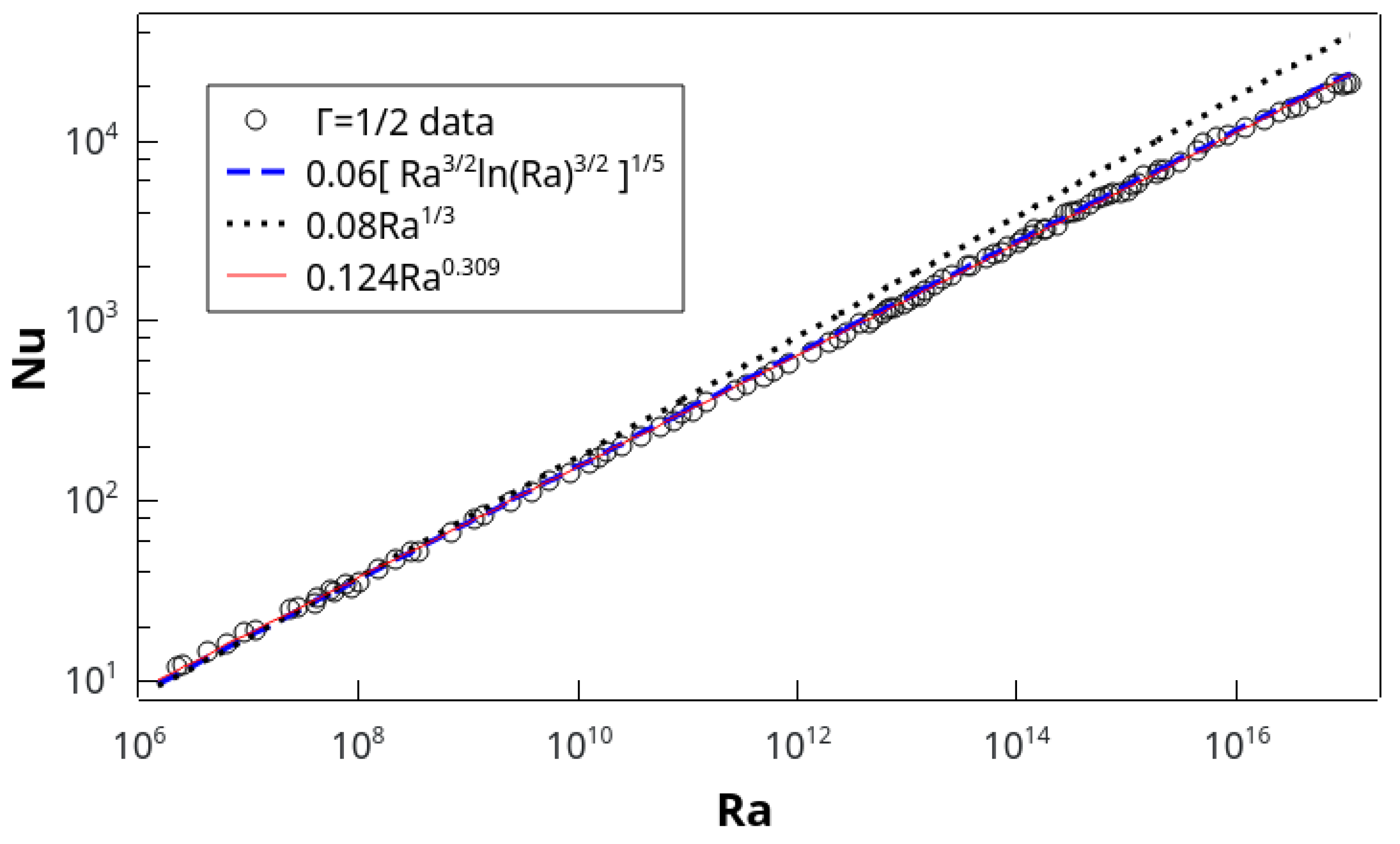
). The fit (see the red dashed line in
Figure 1) is excellent for the entire data. Note that there is no ambiguity in the data that the small difference of the exponent from
is real, perhaps to be regarded as some kind of intermittency correction (see, for example, Ref. [
17]), but there could also be other valid reasons for this slight departure (which could be accounted for by introducing a subleading term). Indeed, numerical simulations at high
in a slender convection cell [
18] suggest an exponent somewhat closer to 1/3, but it certainly appears far from the half-power in
.
In
Figure 1 we also show as the blue dashed line Herring’s prediction for turbulent convection between rigid boundaries, given by Equation (
4), with the prefactor
. The prefactor, the only free parameter in the expression, was obtained by fitting the function to the data. We note that the exponent 0.3 in Equation (
4) is also applied to the ln(
) term so that the effective exponent is slightly larger and, in fact, Herring’s formula fits the data as well as the power-law fit, Equation (
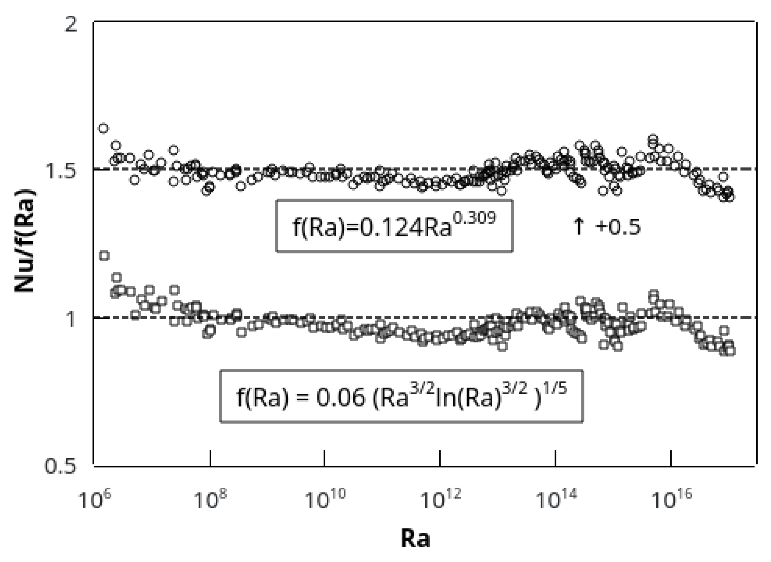
5), as can be seen better in
Figure 2. We emphasize that, instead of two constants of the power law, only the amplitude is an adjustable parameter in Herring’s formula.
In fact,
Figure 2 shows the raw data normalized by both fits and it is clear that each of them is equally good and satisfactory overall. We also note that a considerable substructure to the data exists, which could suggest various changes in the flow, as hinted in the caption to
Figure 2, while preserving the same global trend. We shall give in
Section 5 a brief interpretation of the empirically determined prefactor in Equation (
4).
4. Remarks on the Ultimate State
A brief historical account of the “ultimate” state is provided in the
Appendix A. Here we are content to compare the performance of the Kraichnan formula with those of the other two; see
Figure 3. To bring them all onto one plot, we set
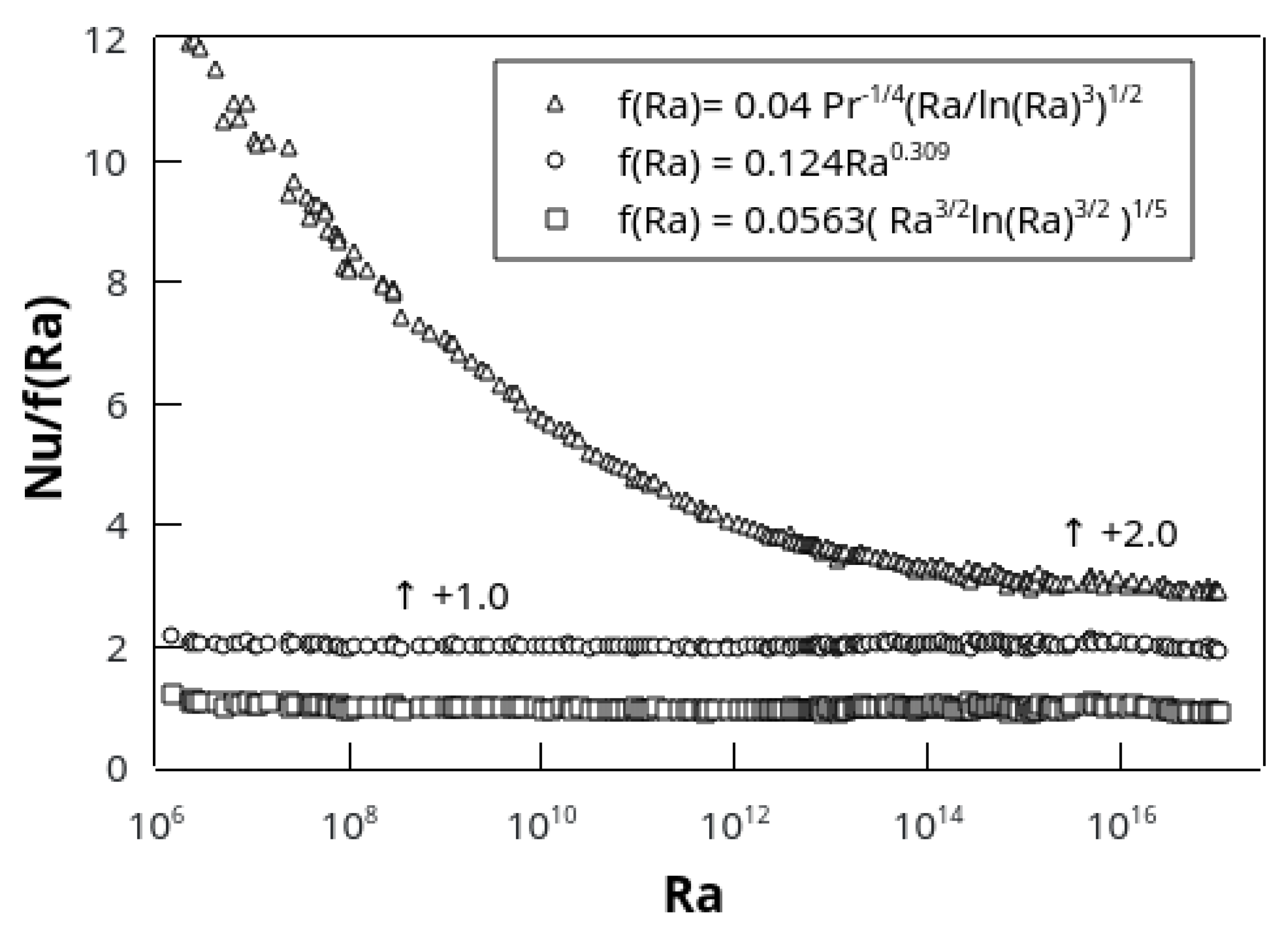
in the Kraichnan formula and compressed the vertical scale by a factor of about 5. On this scale the bottom two fits mask the substructure apparent in
Figure 2 and are almost perfectly straight and horizontal lines, showing that both Equations (4) and (5) work very well from a global perspective. The Kraichnan formula is obviously far from being successful in reducing the data to a horizontal line, so it is clear that it has no global relevance, unlike the other two. However, the curve appears to flatten for high
, tantalizingly suggesting a possible approach to the ultimate state. We shall consider this proposition below.
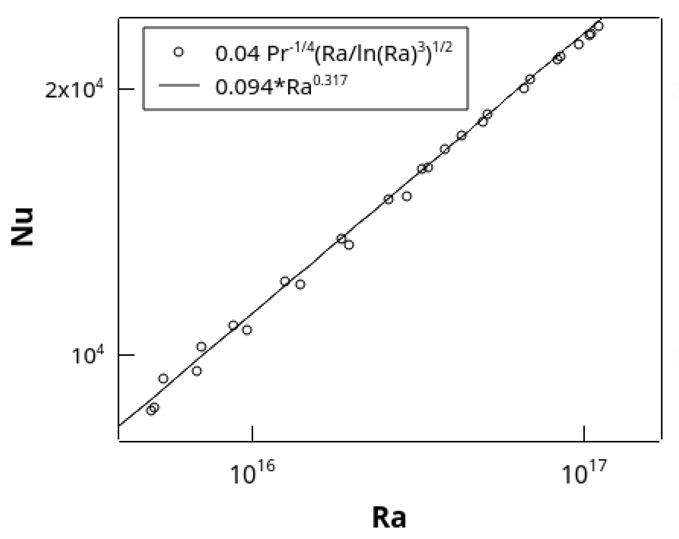
Figure 4 shows an enlarged plot of the Nusselt number against
for the last decade and a half or so. The best fit to those data is a power-law exponent of 0.317, which is only minutely larger (by about 2.5%) than the global exponent of 0.309 (and quite close to the finding in [
18]). No reasonable person would think that the slope is approaching a value of half. From a slightly different perspective,
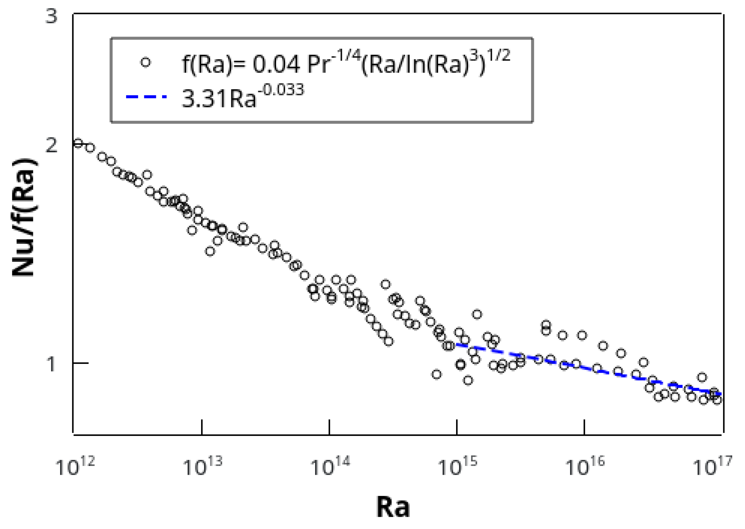
Figure 5 shows the high-
end of the data of
Figure 3; it is clear that the tendency to flatten, which might have been inferred from
Figure 3, is an illusion caused by the compressed scale. It is not clear what functional form the normalized data in
Figure 5 should take, but, if we fit a power law to the last two decades of
, it yields a power law with an exponent of
.
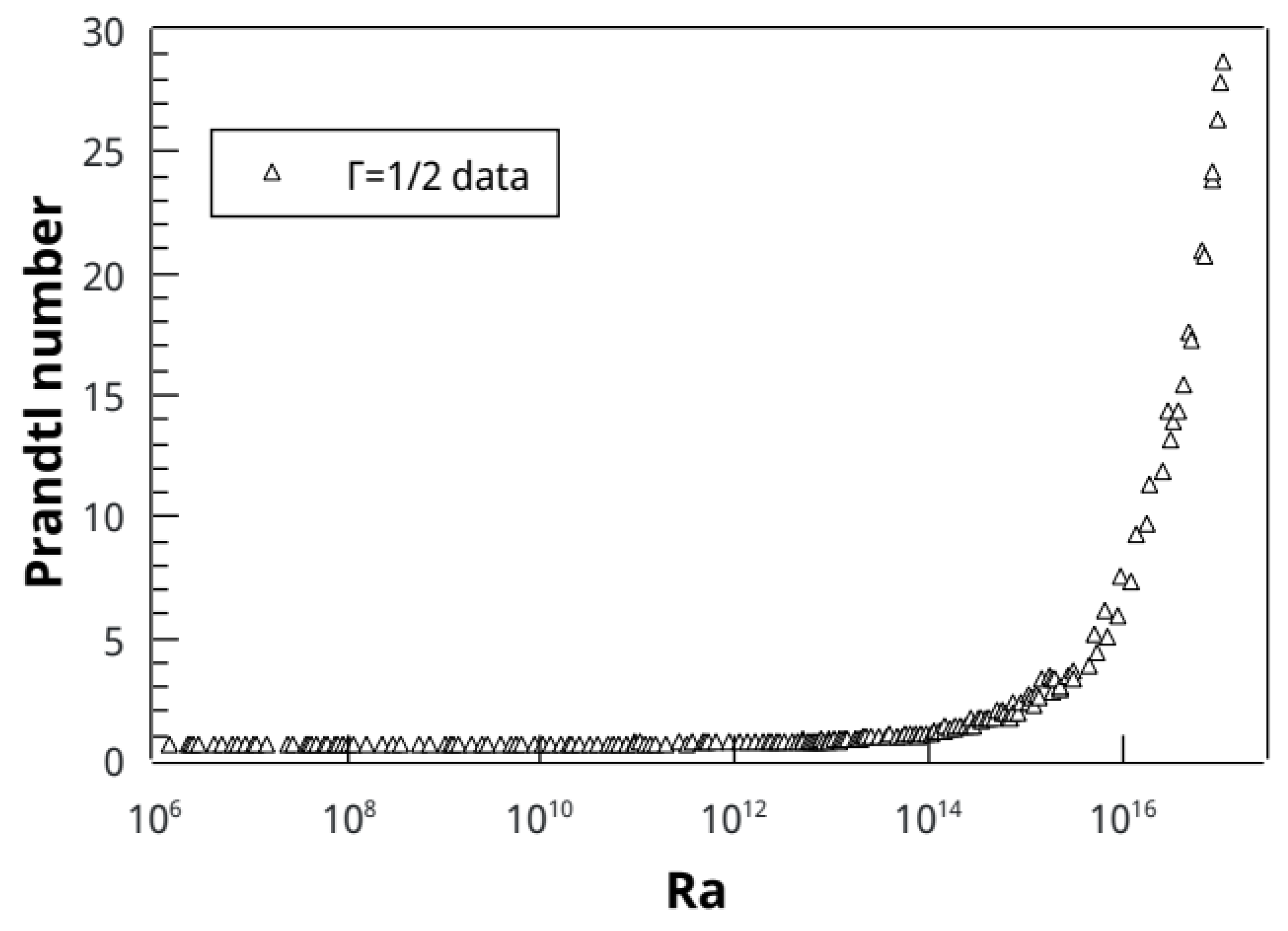
An unstated argument sometimes adduced by the adherents of the ultimate state is to point out that the Prandtl number was not constant in the measurements of [
5] over the last two or so decades of
. This behavior was discussed at length in [
2] and is reproduced in
Figure 6. However, the variation of the Nusselt number on the Prandtl number is very weak for moderate Prandtl numbers in the range encountered here (see, e.g., [
20]). Thus, one cannot argue that the rise in Prandtl number is the reason why the data do not approach the half-power. Our conclusion could be different if the interpretation of the data has the benefit of a precise theory for how the heat transport depends on the Prandtl number.
Figure 3.
normalized according to Equations (4) and (5) as in
Figure 2 but with compressed vertical scale to allow for normalization by Kraichnan’s formula to appear on the same plot. Squares, Nu normalized by Herring’s formula (Equation (
4)). Circles,
normalized by the least-squares fit to the raw data, Equation (
5), with a vertical shift of +1.0 for clarity. Triangles,
normalized according to Kraichnan’s formula for high
and moderate Prandtl number (Equation (
3) with
) with a vertical shift of +2.0 for clarity (see text). Here and in
Figure 5, the dependence on the Prandtl number is left implicit in the notation f(
) as applied to Equation (
3).
Figure 4.
vs.
for the highest decade and a half of
. Symbols:
evaluated using Kraichnan’s formula (Equation (
3) with
). Line: Least-squares fit to the data giving a slope of 0.317.
Figure 4.
vs.
for the highest decade and a half of
. Symbols:
evaluated using Kraichnan’s formula (Equation (
3) with
). Line: Least-squares fit to the data giving a slope of 0.317.
Figure 5.
/f(
) vs.
. The data are normalized using f(
) from Kraichnan’s formula (Equation (
3) with
C = 0.04). Dashed line: least-squares fit to the normalized data for
. The slope over the last two decades is −0.033, indicating that the experimental data do not follow Kraichnan’s formula. The prefactor 3.31 is dependent on the use of
in Equation (
3).
Figure 6.
Prandtl number vs. Rayleigh number for the experiment of Ref. [
5], showing a considerable variation at high
. This variation is an artifact of approaching the critical point of cryogenic helium gas to attain higher and higher Rayleigh numbers. This effect will be even more pronounced if one pushes for high
in a smaller apparatus.
5. Discussion
The discussion here is mainly about two questions. The first question is why Herring’s formula, derived by optimizing the heat transport by single horizontal wavenumber in the slightly nonlinear supercritical regime, should work well for Rayleigh numbers up to . Note that the critical Rayleigh number is 1708 for RBC, and probably higher for this aspect ratio, say a few thousand. Yet the formula seems to apply for an extraordinary range of Rayleigh numbers within which the flow is decidedly turbulent and the range of wavenumbers excited is continuous.
One can perhaps say that this particular success of the Herring formula is a coincidence but that would be an unimaginative stance (given the large number of decades of
over which the agreement occurs). A possible reason for this behavior can perhaps be found in Herring’s 1966 paper [
7], where he states (for free boundaries) that “The physical picture of free boundary convective process predicted by the model is that of a large-scale motion dominating the central region between the conducting plates. This large-scale motion sweeps with it the temperature fluctuation field whose main variations occur in a thin boundary layer of vertical extent 1/
Nu. The horizontal scale of both the dominant motion and the temperature fluctuation field is comparable to the distance between the conducting plates." In actuality, this describes rather well the flow observed between rigid boundaries at high
. Indeed, maintaining the same type of structures at the largest-scale circulation that is present at lower values of supercriticality is not, in fact, unusual (see, for example, ref. [
21] for the case of turbulent wakes). Perhaps not unrelated is the later observation by Krishnamurti and Howard [
22] of a large-scale flow developing and persisting at high
, a phenomenon that has been observed widely in turbulent convection. All of this suggests that the same functional form of the relation appropriate to the weakly nonlinear stage remains valid for the turbulent state, except that the prefactor will be different in the two states. This observation is in the spirit of renormalization. While these ideas are not precise, they have been implemented quantitatively in the isotropic and homogeneous flow generated by Gaussian large-scale forcing [
23]. If this same program can be extended to convection, it would be possible formally to determine the effective transport coefficient. Until that difficult step is completed, the present observation must be regarded as merely suggestive.
The second question concerns the ultimate state. We are aware that half-power occurs in the presence of roughness [
24], when convection occurs in an open-ended tube [
25], when the fluid is heated by a body force such as radiation [
26], etc. For a more complete enumeration of the possible states of convection, see [
27]. As long as the continuum equations hold and the boundary layers on smooth surfaces are intact, it appears to us that their importance to convection will not vanish, and that theories that have no place for viscosity and thermal diffusivity will miss an essential ingredient of the flow. We call attention also to the recent paper by Lindborg [
28], which, with some modifications of Kraichnan’s theory, arrived at the one-third-power. We repeat that, to our knowledge, there is no compelling evidence to date, experimental or numerical, in favor of Kraichnan’s formula. We have made that point explicit with respect to the present data.
