Communication

Ionospheric 14.5 Day Periodic Oscillation during the 2019 Antarctic SSW Event

1
Department of Space Physics, School of Electronic Information, Wuhan University, Wuhan 430072, China
2
Institute of Space Science and Applied Technology, Harbin Institute of Technology, Shenzhen 518055, China
*
Author to whom correspondence should be addressed.
Atmosphere 2023, 14(5), 796; https://doi.org/10.3390/atmos14050796
Submission received: 22 February 2023 / Revised: 17 April 2023 / Accepted: 25 April 2023 / Published: 27 April 2023
(This article belongs to the Special Issue Recent Advances in Ionosphere Observation and Investigation)

Abstract

:
The International Global Navigation Satellite Systems Service (IGS) ionospheric total electron content (TEC) data are used to study the periodic perturbation in the ionosphere during the 2019 Antarctic sudden stratospheric warming (SSW) event, a rare Southern Hemisphere minor SSW event in the last 40 years. A 14.5 day periodic signal with a zonal wavenumber of 0 is observed in the mesosphere and the lower thermosphere (MLT) region and the ionosphere during this SSW period, which could be related to the lunar tide. The 14.5 day periodic disturbance in the IGS TEC exhibits local time dependence and latitudinal variation, with the maximum amplitude appearing between 1000 and 1600 LT in the equatorial ionization anomaly (EIA) crest regions. Additionally, the 14.5 day periodic oscillation shows an obvious longitudinal variability, with the weakest amplitude appearing in the longitudinal region of 30° W–60° E.

1. Introduction

Sudden stratospheric warming (SSW) is one of the large-scale meteorological phenomena in the stratosphere of the winter hemisphere over the polar region, and is accompanied by dramatic changes in temperature, wind, and the polar vortex [1,2,3]. The key mechanism of SSW formation is attributed to the amplified upward propagation of stationary planetary waves from the troposphere and their nonlinear interaction with the mean flow in the stratosphere [4]. In addition to the enhanced planetary waves from the troposphere, enhanced gravity wave drag in the polar night jet is found to be important for the split of SSWs [5]. Based on reanalysis data, Albers and Birner (2014) also found that apart from the planetary wave forcing from the troposphere, there is another theory for the occurrence of the SSWs called resonance. In this theory, the SSW can occur even without anomalous planetary wave forcing from the troposphere. If SSWs are triggered by resonance, then “preconditioning” is interpreted as the basic state constraints that “tune” the vortex into a geometric structure that supports resonance.
Long-term observations indicate that SSW events are rare in the southern hemisphere (SH), mainly due to the lower topography and a lower land–sea contrast, resulting in weaker planetary wave forcing in the SH. Based on changes in the stratospheric circulation and timing, SSW events are classified as major and minor. Following the standard World Meteorological Organization (WMO) definition [6], a “minor warming” is identified when polar temperatures increase by 25 K or more within a week at any stratospheric level. In a major warming, the zonal mean zonal wind at 60° N and 10 hPa reverses from westerly to easterly [7].
Although SSW events occur in the stratosphere of the winter hemisphere over the polar region, they strongly affect the vertical coupling in a large range of altitudes up to the thermosphere [8]. In addition, their effects are not limited to high latitudes, but penetrate into low latitudes or even to the opposite hemisphere. Anomalies in the stratosphere winter hemisphere are linked to anomalies in the summer mesosphere, which is called interhemispheric coupling [9]. Becker et al. (2004) modeled the response of the northern hemisphere in the summer of 2002 to enhanced planetary wave activity at high southern latitudes. This study suggested higher temperatures and a weaker residual mean (vertical and meridional) circulation near the mesopause, with lower temperatures and a stronger residual circulation in the middle mesosphere [10]. Numerical observational studies have revealed the effects of SSW on various ionospheric parameters, such as total electron content (TEC) [11,12,13], peak electron density (foF2) [14,15], electric fields [16,17] and vertical plasma drift [18]. Satellite measurements further revealed the global ionospheric variability during SSW periods [15,19]. Numerical observations and simulations demonstrated that ionospheric disturbances in the low–middle latitudes and equatorial regions during an SSW period are attributed to the modulation in vertical plasma drift by the nonlinear interaction between planetary waves and tides and the direct impact of tidal waves [20,21,22]. At mid–high latitudes, changes in the thermospheric neutral composition and background wind caused by tide- and SSW-driven circulation are important sources of ionospheric perturbation during SSW periods [15,23,24].
The enhanced lunar tidal impact on ionospheric variations during SSW events has attracted the interest of many researchers. Both observations [25,26] and simulations [22,27] reveal that the enhancement in lunar tides during SSW periods is due to changes in the mean zonal winds in the stratosphere and mesosphere [26,27]. Park et al. (2012) found that the equatorial electrojet shows an enhanced 13-day modulation and ascribed it to the lunar tidal modulation [28]. Mo and Zhang (2018) revealed that the location of the equatorial ionization anomaly (EIA) crest presents an obvious and constant 14 to 15 day periodic disturbance during SSW events, attributing this perturbation to the enhanced lunar tide modulated by the zonal wind [29]. In a recently published paper, Tang et al. (2021) found a strong 14.5 day oscillation in the critical frequency of the F2 region during the 2014–2015 SSW event [30].
Apart from the PWs, previous studies have revealed that geomagnetic activities can also generate planetary wave-type signatures with periods of 5, 10, and 13.5 days in the ionosphere [31,32,33]. Furthermore, oscillations of multi-day periods (near 5.5, 7 and 9 day subharmonics of the solar rotation) associated with recurrent high speed solar wind streams were discovered in the thermosphere and TEC as well [34,35,36] (Lei et al., 2008a, 2008b, 2008c; Mlynczak et al., 2008; Thayer et al., 2008).
In September 2019, a rare SSW event occurred in the SH. The last SSW that occurred in the SH was in 2002. Compared with the SSW event occurring in the northern hemisphere, although the 2019 SSW was classified as minor, according to the standard WMO definition, it was accompanied by the smallest Antarctic ozone hole on record [37]. Lossow et al. (2011) found that strengthened stratospheric westerlies arising from the ozone hole led to a reduced eastward gravity wave drag in the mesosphere and a warming of the polar mesosphere [38]. Furthermore, Omrani et al. (2016) proved that the strengthened stratospheric westerlies arising from the cooling induced by the Antarctic ozone hole causes a polar mesospheric warming and a subsequent cooling in the lower thermosphere [39].
The characteristics of the quasi-6-day perturbation in the ionosphere during the 2019 Antarctic SSW have been extensively investigated [40,41,42]. For instance, based on the International Global Navigation Satellite Systems Service (IGS) TEC maps, Gu et al. (2021) investigated the global characteristic of the quasi-6-day disturbance in the ionosphere [41]. However, perturbations with other periods in the ionosphere have rarely been studied during the 2019 Antarctic SSW. As mentioned above, the enhanced lunar tide and its effects on the ionosphere during SSW periods have been revealed by many researchers. In this paper, we aim to study the global characteristics of the 14–15 day periodic oscillation in the ionosphere during this rare SSW event. Section 2 presents the datasets and the method. The global features of the 14.5 day oscillation in the ionospheric TEC are presented in Section 3. The discussion and summary are given in Section 4.

2. Datasets and Analysis Method

2.1. Datasets

The temperature and wind data provided by the National Centers for Environmental Prediction/National Center of Atmospheric Research (NCEP/NCAR) reanalysis datasets were used to analyze the features of the 2019 Antarctic SSW event.
The TIMED Doppler Interferometer (TIDI) instrument onboard the TIMED satellite aims to measure winds in the mesosphere and the lower thermosphere (MLT) region [43]. TIDI data cover the height range of 60–300 km. TIDI winds have been widely used to analyze atmospheric waves such as planetary waves and tides in the MLT region [44,45].
Based upon observations of the widely distributed network of ground-based Global Positioning System (GPS) receivers, the IGS routinely provides a global TEC map with 2.5° × 5° latitude–longitude grids and a 0.25 h UT resolution. The TEC maps provide global information on the ionosphere, which enables investigating the global ionospheric response to the 2019 Antarctic SSW event.

2.2. Analysis Method

In this work, the least squares fitting method was utilized to calculate the periodic signal in the TIDI winds [46].
y = A cos 2 π t d + t u T s λ + B sin 2 π · t d + t u T s λ + C
where T is the period in days, td is the day of the year, tu is the universal time in days, s is the zonal wave number and λ is the longitude (in radians) normalized by 2π.
The period was varied from 10 to 18 days with a step of 0.2 days during processing to determine the spectra of the measurements and the amplitudes of the periodic signal. A (B) is the coefficient of the cosine (sine) term and C represents the background value. The amplitude of the period signal is expressed as:
R 2 T , s = A 2 T , s + B 2 T , s
To calculate the wavenumber–period spectra of the TIDI zonal wind, an analysis was performed within ±5° latitude of the special latitude.
Due to the photochemistry of solar radiation, the ionosphere dramatically varies from daytime to nighttime; the extraction of periodic signals in the ionospheric parameters is hence more complicated. Thus, the TEC observations at different local times were analyzed separately. Then, Equation (1) can be written as [46]:
y = A cos 2 π t d + t L λ T s λ + B sin 2 π · t d + t L λ T s λ + C
where t u = t L λ · 360 15 × 24 = t L λ . The amplitude is expressed as:
R 2 T , s , L = A 2 T , s , L + B 2 T , s , L

3. Results

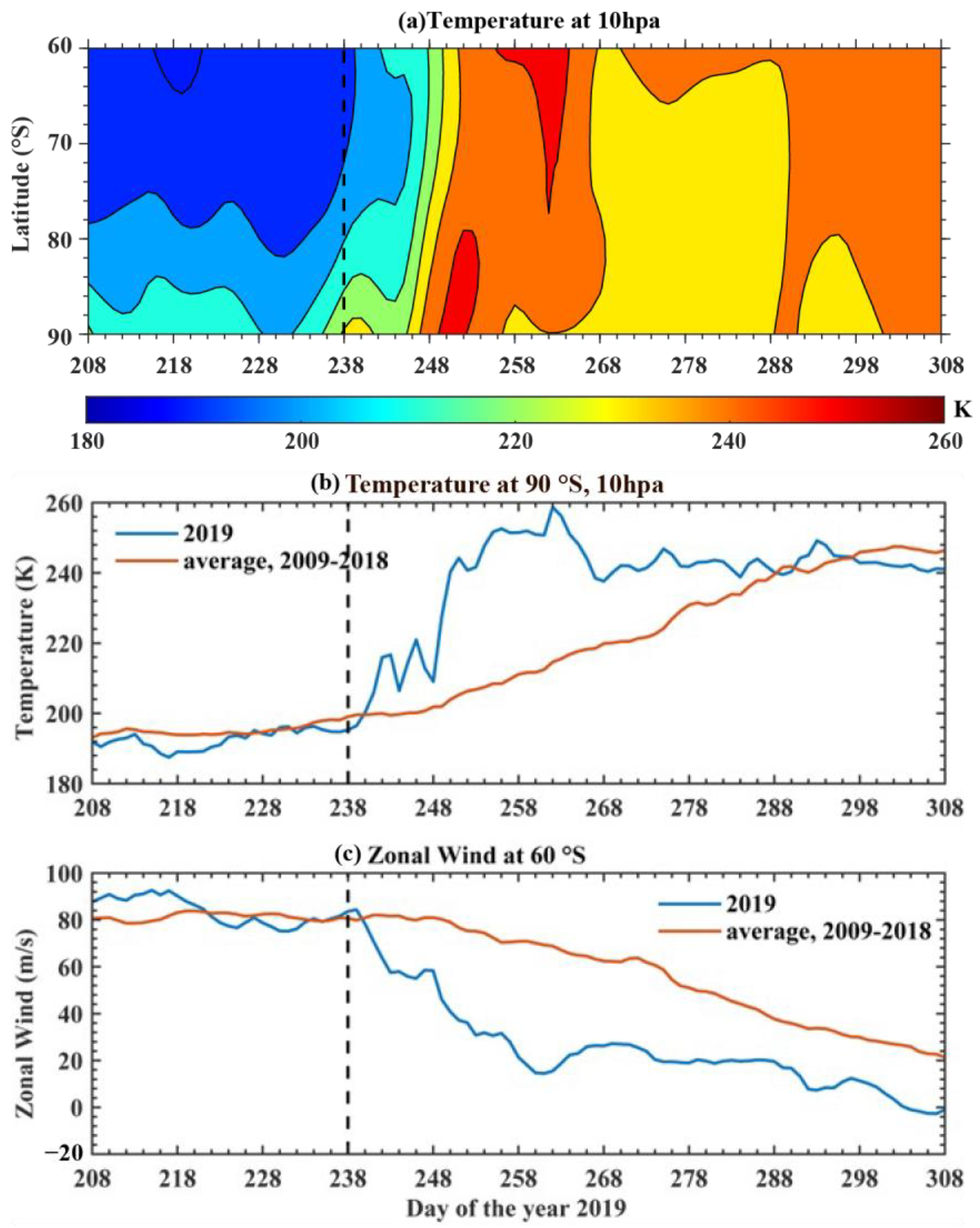
3.1. Minor SH SSW in 2019 and 14.5 Day Oscillation in the Neutral Atmosphere

Figure 1 presents the variations in the stratospheric temperature and stratospheric wind from DOY (day of the year) 208 to 308 in 2019. Figure 1a shows the temperature at 10 hPa from 60° S to 90° S. The temperature increased after DOY 238. We can see from Figure 1b that the stratospheric temperature increased from 196 K on DOY 238 (highlighted by the black dashed line), indicating the warming onset, to a maximum of 260 K on DOY 260. The 10 year averages from 2009 to 2018 are shown by the red solid lines. The temperature increased by more than 60 K. The stratospheric wind decreased but did not reverse during the warming period, as shown in Figure 1c; therefore, the 2019 Antarctic SSW is defined as a minor SSW according to the WMO definition. The increase in temperature lasted for about 3 weeks, and then recovered to the mean on DOY 288.
The wavenumber–period spectra of the zonal wind at 97.5 km and 10° N and 10° S during DOY 238–298 in 2019 are exhibited in Figure 2. A periodic signal centering at 14.5 days with a zonal wavenumber of 0 is seen in the zonal wind. The wavenumber 0 indicates that the 14.5 day periodic signal is just an oscillation that cannot propagate in the zonal direction.

3.2. Geomagnetic and Solar Activities during SH Winter in 2019

Geomagnetic and solar activities play a significant role in ionospheric variability, and periodic oscillations of the ionosphere caused by the geomagnetic and solar activities have been investigated by many researchers [31,32,33]. Thus, it is necessary to examine the periodicity of geomagnetic and solar indexes before analyzing the periodic signal in the ionosphere during the 2019 Antarctic SSW period. Figure 3a,b shows the variation in the geomagnetic Dst and solar F10.7 indexes (solar flux at 10.7 cm wavelength) with error bars during the period from DOY 208 to 298. The solar F10.7 index remained relatively constant at ~65–75 sfu, representing a solar minimum and quiet conditions. The Dst index decreased from 0 nT on DOY 242 and reached a minimum of −40 nT on DOY 245 in 2019, indicating a minor geomagnetic storm occurring during the 2019 Antarctic SSW. The wavelet spectra of the Dst and F10.7 indexes are presented in Figure 3c,d. Periodic signals with a period of 14.5 days are not observed in periodograms of both indexes, which suggests that the 14.5 day signal in the ionosphere during the 2019 SSW period is not due to geomagnetic or solar activities.
As shown in Figure 2, there is an obvious 14.5 day periodic signal in the MLT region during the 2019 Antarctic SSW period. Meanwhile, the solar and geomagnetic indices do not exhibit a 14.5 day periodic signal during the same period, as presented in Figure 3. This encourages us to examine whether this is the same periodic signal in the ionosphere during the 2019 SSW period. Figure 4 shows the wavenumber–period spectra of the IGS TEC at 10° N and 10° S during the SSW event. Similar to the spectra in the TIDI wind, a 14.5 day periodic signal with a zonal wavenumber of 0 is also observed in the IGS TEC.

3.3. Equatorial Ionospheric Response to 2019 SSW in the SH

Then, the global ionospheric responses to the 2019 Antarctic SSW event were investigated based on the IGS TEC maps. Since the IGS TEC maps are reconstructed data based on the observations at PGS stations, grids with more data coverage were chosen. Figure 5a,b shows the spectra of the IGS TEC at (115° E, 10° N) and (75° W, 10° N) during the SSW period. The 14.5 day periodic oscillation dominates the spectra from 1000 to 1600 LT (local time). The latitudinal local time variations in the 14.5 day periodic oscillation amplitudes at 115° E and 75° W during the SSW period are shown in Figure 5c,d, and two obvious enhancements occur during 1000–1600 LT in the EIA crest regions. Figure 5e,f shows the latitudinal local time structure of the mean background TEC at 115° E and 75° W. The background mean TEC shows the maximum in the EIA crest regions during 1000–2000 LT. Note that the appearance of peaks of the 14.5 day perturbation is about two hours before that of the background mean TEC.
Apart from the prominent latitudinal variations in the ionosphere, studying longitudinal variations is also important. Figure 6 presents the latitudinal distribution of the TEC spectra at 1200 LT at different longitudes during the SSW period. The TEC spectra show a 14.5 day periodic oscillation at most longitudinal sites in the EIA crest regions. Additionally, the amplitude of the 14.5 day periodic oscillation in the IGS TEC presents clear longitudinal features, with the minimum appearing in the longitudinal zone of 30° W–60° E, and the maximum occurring in the longitudinal zone from 150° W to 60° W.
Figure 7a shows the longitude–latitude distribution of the 14.5 day period amplitude in the IGS TEC at 1200 LT during the SSW period. It is clear that the 14.5 day oscillation shows two maxima on the northern and southern sides of the geomagnetic equator (magnetic latitudes of 15° N and 15° S). Additionally, the 14.5 day oscillation of the ionosphere displays an obvious longitudinal structure, with the minimum appearing in the longitudinal region of 30° W–60° E and the maximum occurring in the longitudinal zones of 180–120° W and 90–60° W. Figure 7b presents the latitudinal–longitudinal distribution of the mean background IGS TEC at 1200 LT. The longitudinal region of the minimum 14.5 day oscillation in the IGS TEC is consistent with that of the minimum mean background TEC. However, the inconsistency between the 14.5 day oscillation and the mean background IGS TEC cannot be ignored, for instance, the mean background TEC is strong in the longitudinal region of 60–120° E, while the 14.5 day oscillation in this region is weak.

4. Discussion and Summary

In this study, the global characteristics of the 14.5 day periodic oscillation in the ionospheric IGS TEC are investigated. Our results demonstrate the presence of a 14.5 day periodic signal with a zonal wavenumber of 0 in the MLT region and the ionosphere during the 2019 Antarctic SSW event. This 14–15 day periodic oscillation has been previously reported by many researchers. For example, Mo and Zhang (2018) demonstrated the presence of a 14–15 day periodic oscillation in the location of EIA crests in both China and Brazilian regions during SSW events, which is in good agreement with the half lunar month [29]. Tang et al. (2021) also found an enhanced semi-monthly lunar tide oscillation (~14.5 day period) in the critical frequency of the F2 region in the EIA crests during the 2014–2015 SSW event [30]. Forbes and Zhang (2012) showed that the underlying mechanism for lunar tidal enhancement during the SSW event was due to changes in the zonal-mean temperature and wind structure of the middle atmosphere that occurred during the SSW [26]. The occurrence of SSWs is accompanied by dramatic changes in temperature, wind and polar the vortex [1,2,3].
As shown in Figure 5, the 14.5 day periodic oscillation in the IGS TEC exhibits a clear local time dependence, with the maximum amplitude appearing between 1000 and 1600 LT. In this study, the 14.5 day periodic perturbation in the ionosphere has been attributed to the lunar tide. The local time features of the lunar tide have been investigated by many researchers [12,47]. For instance, Yamazaki (2013) revealed that the lunar tide shows obvious local time variations, with the maximum occurring between 0900 and 1600 LT. Moreover, an enhanced lunar tide during the SSW period has also been found by many researchers [47]. This indicates that the local time variation of the 14.5 day perturbation could be attributed to the effects of the lunar tide.
As shown in Figure 5 and Figure 6, the 14.5 day periodic perturbation is evident in the IGS TEC, peaking at EIA crests. The latitudinal structure of the 14.5 day periodic oscillation is similar to the quasi-6 day disturbance in the ionosphere during the 2019 Antarctic SSW event [34,48]. Lin et al. (2020) attributed the latitudinal structure of the quasi-6 day disturbance to a modulation in the equatorial ionospheric fountain effect [42]. Pedatella and Forbes (2010) examined the global structure of lunar tides and found that the semidiurnal lunar tide achieves maximum amplitude in the EIA crest regions [12]. Therefore, we suggest that the latitudinal variation in the 14.5 day periodic perturbation is also due to the modulation in the fountain effect by the lunar tidal wind.
In addition to the significant latitudinal variation in the 14.5 day period, a longitudinal variation is also obvious. As shown in Figure 6 and Figure 7, the 14.5 day periodic oscillation is generally weaker in the longitudinal region between 30° W and 60° E. Recently, Goncharenko et al. (2020) revealed that the ionospheric response to this 2019 SSW event was dramatic in the longitudinal structure, including in the periodical signals [40]. They attributed the longitudinal variations in the ionosphere to the modulation in the non-migrating diurnal tide. In this study, we attribute the 14.5 day periodic perturbation both in the neutral atmosphere (demonstrated by the MLT wind) and ionosphere (demonstrated by the TEC) to the lunar tides. A significant longitudinal variability in the semidiurnal lunar tide has been revealed by Yamazaki et al. (2017) [49]. This suggests that the longitudinal structure of the 14.5 day periodic oscillation could be related to the longitudinal features of the lunar tide.
This study investigated the 14.5 day periodic oscillation in the TEC during the 2019 Antarctic SSW event. The main results are summarized as follows:
(1)
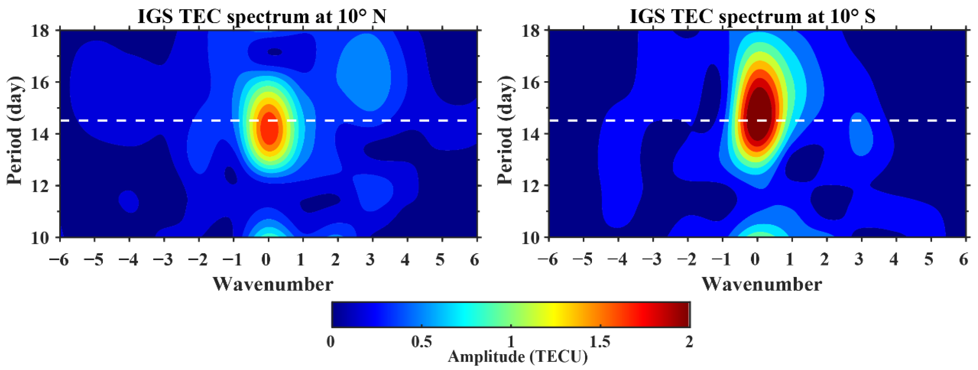
During the 2019 Antarctic SSW event, a 14.5 day period signal with a zonal wavenumber of 0 is observed both in the neutral atmosphere (demonstrated by the MLT wind) and ionosphere (demonstrated by the TEC).
(2)
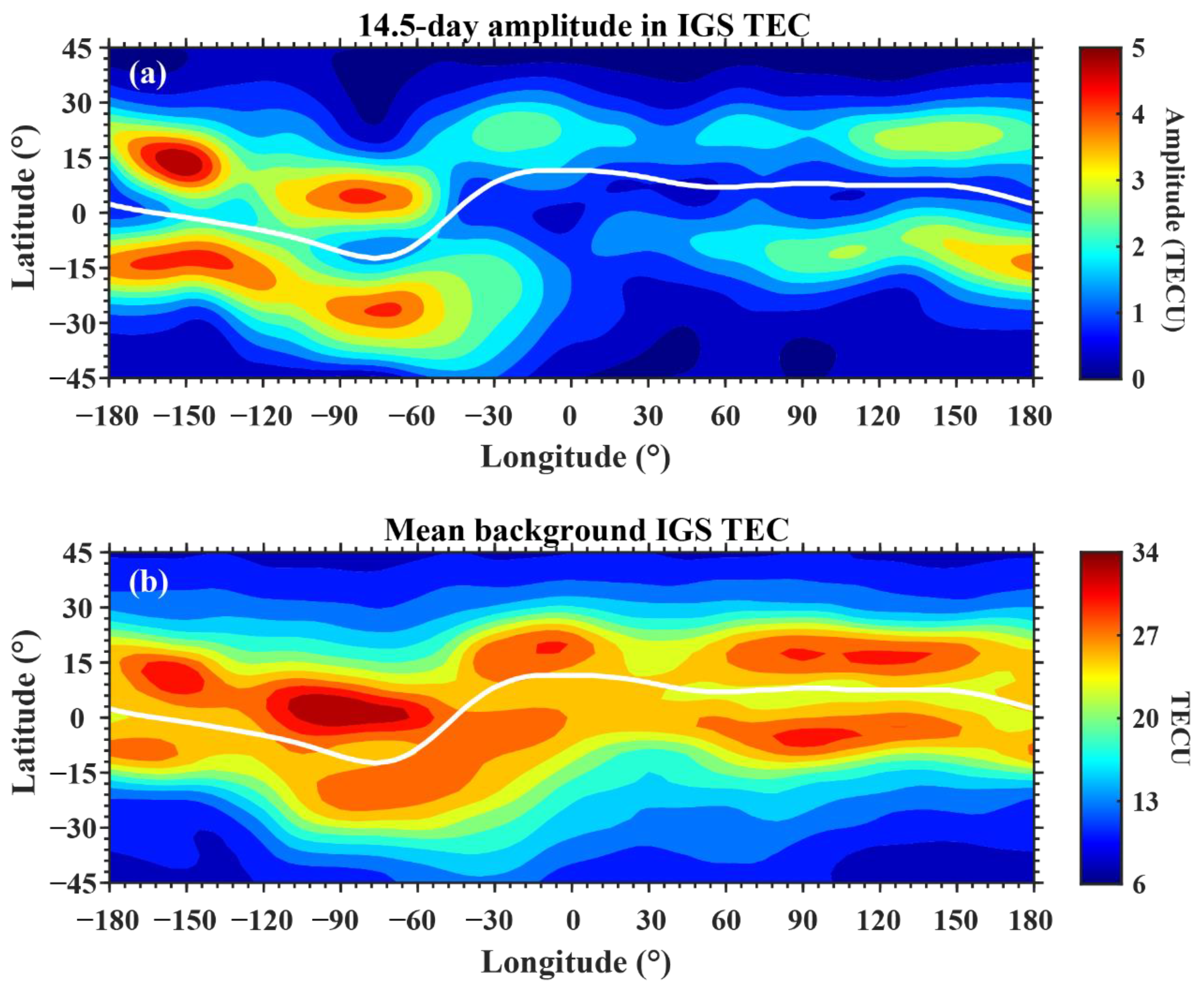
The 14.5 day periodic oscillation in the ionosphere shows significant latitudinal variation with the maximum amplitude occurring at EIA crests.
(3)
The 14.5 day periodic oscillation in the ionosphere shows local time dependence, with the maximum amplitude appearing in the time range from 1000 to 1600 LT.
(4)
The 14.5 day periodic oscillation is generally weaker in the longitudinal region between 30° W and 60° E.

Author Contributions

Methodology and investigation, C.Z. and Q.T.; data curation and writing—original draft preparation, J.L.; writing—review and editing, Q.T., Y.W. and Y.L. All authors have read and agreed to the published version of the manuscript.

Funding

This research was funded by the National Natural Science Foundation of China (nos. 41574146, 41774162, 42004130, 42204161 and 42104150), the fellowship of China Postdoctoral Science Foundation (2022M710941), the Foundation of National Key Laboratory of Electromagnetic Environment (grant nos. 6142403180204 and 6142403200303), the Chinese Academy of Sciences, the Key Laboratory of Geospace Environment, University of Science & Technology of China (GE2020-01) and the Fundamental Research Funds for the Central Universities (2042021kf0020).

Data Availability Statement

The IGS TEC map can be downloaded at https://www.igs.org/products-access/#atmospheric-parameters (accessed on 13 December 2022). The TIDI measurements can be downloaded at http://download.hao.ucar.edu/archive/tidi/ (accessed on 13 December 2022). NCEP data can be downloaded at https://psl.noaa.gov/data/gridded/data.ncep.reanalysis.html (accessed on 13 December 2022). Solar and geomagnetic indexes can be downloaded at https://omniweb.gsfc.nasa.gov/form/dx1.html (accessed on 13 December 2022).

Acknowledgments

We acknowledge the use of TEC data from the International Global Navigation Satellite Systems Service (IGS). We also appreciate the TIDI data provided by the National Center for Atmospheric Research.

Conflicts of Interest

The authors declare no conflict of interest.

Abbreviations

Full TermAbbreviation
Sudden Stratospheric WarmingSSW
Southern HemisphereSH
Total Electron ContentTEC
Peak Electron DensityfoF2
Equatorial Ionization AnomalyEIA
Northern HemisphereNH
International Global Navigation Satellite Systems ServiceIGS
National Centers for Environmental Prediction/National Center of Atmospheric ResearchNCEP/NCAR
The TIMED Doppler InterferometerTIDI
Mesosphere and the Lower ThermosphereMLT
Global Positioning SystemGPS
Local TimeLT

References

  1. Andrews, D.G.; Holton, J.R.; Leovy, C.B. Middle Atmosphere Dynamics; Academic Press: San Diego, CA, USA, 1987. [Google Scholar]
  2. Butler, A.H.; Seidel, D.J.; Hardiman, S.C.; Butchart, N.; Birner, T.; Match, A. Defining Sudden Stratospheric Warmings. Bull. Am. Meteorol. Soc. 2015, 96, 1913–1928. [Google Scholar] [CrossRef]
  3. Chandran, A.; Collins, R.L. Stratospheric sudden warming effects on winds and temperature in the middle atmosphere at middle and low latitudes: A study using WACCM. Ann. Geophys. 2014, 32, 859–874. [Google Scholar] [CrossRef]
  4. Matsuno, T. A Dynamical Model of the Stratospheric Sudden Warming. J. Atmos. Sci. 1971, 28, 1479–1494. [Google Scholar] [CrossRef]
  5. Albers, J.R.; Birner, T. Vortex Preconditioning due to Planetary and Gravity Waves prior to Sudden Stratospheric Warmings. J. Atmos. Sci. 2014, 71, 4028–4054. [Google Scholar] [CrossRef]
  6. McInturff, R.M. Stratospheric Warmings: Synoptic, Dynamic and General-Circulation Aspects. (1978). Available online: https://ntrs.nasa.gov/archive/nasa/casi.ntrs.nasa.gov/19780010687 (accessed on 3 September 2013).
  7. Yamazaki, Y.; Matthias, V.; Miyoshi, Y.; Stolle, C.; Siddiqui, T.; Kervalishvili, G.; Laštovička, J.; Kozubek, M.; Ward, W.; Themens, D.R.; et al. September 2019 Antarctic Sudden Stratospheric Warming: Quasi-6-Day Wave Burst and Ionospheric Effects. Geophys. Res. Lett. 2020, 47, e2019GL086577. [Google Scholar] [CrossRef]
  8. Liu, H.-L.; Roble, R.G. A study of a self-generated stratospheric sudden warming and its mesospheric-lower thermospheric impacts using the coupled TIME-GCM/CCM3. J. Geophys. Res. 2002, 107, 4695. [Google Scholar] [CrossRef]
  9. Goldberg, R.A.; Fritts, D.C.; Williams, B.P.; Lübken, F.; Rapp, M.; Singer, W.; Latteck, R.; Hoffmann, P.; Müllemann, A.; Baumgarten, G.; et al. The MaCWAVE/MIDAS rocket and ground-based measurements of polar summer dynamics: Overview and mean state structure. Geophys. Res. Lett. 2004, 31, L24S02. [Google Scholar] [CrossRef]
  10. Becker, E.; Müllemann, A.; Lübken, F.J.; Körnich, H.; Hoffmann, P.; Rapp, M. High Rossby-wave activity in austral winter 2002: Modulation of the general circulation of the MLT during the MaCWAVE/MIDAS northern summer program. Geophys. Res. Lett. 2004, 31, L24S03. [Google Scholar] [CrossRef]
  11. Chau, J.L.; Aponte, N.A.; Cabassa, E.; Sulzer, M.P.; Goncharenko, L.; Gonzalez, S.A. Quiet time ionospheric variability over Arecibo during sudden stratospheric warming events. J. Geophys. Res. 2010, 115, 1–8. [Google Scholar] [CrossRef]
  12. Pedatella, N.M.; Forbes, J.M. Evidence for stratosphere sudden warming-ionosphere coupling due to vertically propagating tides. Geophys. Res. Lett. 2010, 37, L11104. [Google Scholar] [CrossRef]
  13. Sridharan, S. Variabilities of Low-Latitude Migrating and Nonmigrating Tides in GPS-TEC and TIMED-SABER Temperature during the Sudden Stratospheric Warming Event of 2013. J. Geophys. Res. Space Phys. 2017, 122, 10748–10761. [Google Scholar] [CrossRef]
  14. Pancheva, D.; Mukhtarov, P. Stratospheric warmings: The atmosphere–ionosphere coupling paradigm. J. Atmos. Sol.-Terr. Phys. 2011, 73, 1697–1702. [Google Scholar] [CrossRef]
  15. Yue, X.; Schreiner, W.S.; Lei, J.; Rocken, C.; Hunt, D.C.; Kuo, Y.-H.; Wan, W. Global ionospheric response observed by COSMIC satellites during the January 2009 stratospheric sudden warming event. J. Geophys. Res. 2010, 115, A00G09. [Google Scholar] [CrossRef]
  16. Anderson, D.; Araujo-Pradere, E.A. Sudden stratospheric warming event signatures in daytime ExB drift velocities in the Peruvian and Philippine longitude sectors for January 2003 and 2004. J. Geophys. Res. 2010, 115, A00G05. [Google Scholar] [CrossRef]
  17. Fejer, B.G.; Olson, M.E.; Chau, J.; Stolle, C.; Luhr, H.; Goncharenko, L.; Yumoto, K.; Nagatsuma, T. Lunar-dependent equatorial ionospheric electrodynamic effects during sudden stratospheric warmings. J. Geophys. Res. 2010, 115, A07314. [Google Scholar] [CrossRef]
  18. Chau, J.L.; Fejer, B.G.; Goncharenko, L.P. Quiet variability of equatorial E × B drifts during a sudden stratospheric warming event. Geophys. Res. Lett. 2009, 36, L05101. [Google Scholar] [CrossRef]
  19. Korenkov, Y.N.; Klimenko, V.V.; Bessarab, F.S.; Korenkova, N.A.; Ratovsky, K.G.; Chernigovskaya, M.A.; Shcherbakov, A.A.; Sahai, Y.; Fagundes, P.R.; De Jesus, R.; et al. The global thermospheric and ionospheric response to the 2008 minor sudden stratospheric warming event. J. Geophys. Res. 2012, 117, A10309. [Google Scholar] [CrossRef]
  20. Goncharenko, L.P.; Chau, J.L.; Liu, H.-L.; Coster, A.J. Unexpected connections between the stratosphere and ionosphere. Geophys. Res. Lett. 2010, 37, L10101. [Google Scholar] [CrossRef]
  21. Liu, H.X.; Yamamoto, M.; Ram, S.T.; Tsugawa, T.; Otsuka, Y.; Stolle, C.; Doornbos, E.; Yumoto, K.; Nagatsuma, T. Equatorial electrodynamics and neutral background in the Asian sector during the 2009 stratospheric sudden warming. J. Geophys. Res. Atmos. 2011, 116, A08308. [Google Scholar] [CrossRef]
  22. Pedatella, N.M.; Liu, H.-L. The influence of atmospheric tide and planetary wave variability during sudden stratosphere warmings on the low latitude ionosphere. J. Geophys. Res. Space Phys. 2013, 118, 5333–5347. [Google Scholar] [CrossRef]
  23. Pedatella, N.M.; Richmond, A.D.; Maute, A.; Liu, H.L. Impact of semidiurnal tidal variability during SSWs on the mean state of the ionosphere and thermosphere. J. Geophys. Res. Space Phys. 2016, 121, 8077–8088. [Google Scholar] [CrossRef]
  24. Yasyukevich, A.S. Variations in Ionospheric Peak Electron Density during Sudden Stratospheric Warmings in the Arctic Region. J. Geophys. Res. Space Phys. 2018, 123, 3027–3038. [Google Scholar] [CrossRef]
  25. Chau, J.L.; Hoffmann, P.; Pedatella, N.M.; Matthias, V.; Stober, G. Upper mesospheric lunar tides over middle and high latitudes during sudden stratospheric warming events. J. Geophys. Res. Space Phys. 2015, 120, 3084–3096. [Google Scholar] [CrossRef]
  26. Forbes, J.M.; Zhang, X. Lunar tide amplification during the January 2009 stratosphere warming event: Observations and theory. J. Geophys. Res. 2012, 117, A12312. [Google Scholar] [CrossRef]
  27. Jin, H.; Miyoshi, Y.; Pancheva, D.; Mukhtarov, P.; Fujiwara, H.; Shinagawa, H. Response of migrating tides to the stratospheric sudden warming in 2009 and their effects on the ionosphere studied by a whole atmosphere-ionosphere model GAIA with COSMIC and TIMED/SABER observations. J. Geophys. Res. 2012, 117, A10323. [Google Scholar] [CrossRef]
  28. Park, J.; Lühr, H.; Kunze, M.; Fejer, B.G.; Min, K.W. Effect of sudden stratospheric warming on lunar tidal modulation of the equatorial electrojet. J. Geophys. Res. 2012, 117, A03306. [Google Scholar] [CrossRef]
  29. Mo, X.H.; Zhang, D.H. Lunar Tidal Modulation of Periodic Meridional Movement of Equatorial Ionization Anomaly Crest during Sudden Stratospheric Warming. J. Geophys. Res. Space Phys. 2018, 123, 1488–1499. [Google Scholar] [CrossRef]
  30. Tang, Q.; Zhou, C.; Li, Z.; Liu, Y.; Chen, G. Semi-Monthly Lunar Tide Oscillation of foF2 in Equatorial Ionization Anomaly (EIA) Crests during 2014–2015 SSW. J. Geophys. Res. Space Phys. 2021, 126, e2020JA028708. [Google Scholar] [CrossRef]
  31. Altadill, D.; Apostolov, E.M. Vertical propagating signatures of wave-type oscillations (2- and 6.5-days) in the ionosphere obtained from electron-density profiles. J. Atmos. Sol.-Terr. Phys. 2001, 63, 823–834. [Google Scholar] [CrossRef]
  32. Altadill, D.; Apostolov, E.M. Time and scale size of planetary wave signatures in the ionosphere F region: Role of the geomagnetic activity and mesosphere/lower thermosphere winds. J. Geophys. Res. 2003, 108, 1403. [Google Scholar] [CrossRef]
  33. Xiong, J.; Wan, W.; Ning, B.; Liu, L.; Gao, Y. Planetary wave-type oscillations in the ionosphere and their relationship to mesospheric/lower thermospheric and geomagnetic disturbances at Wuhan (30.6°N, 114.5°E). J. Atmos. Sol.-Terr. Phys. 2005, 68, 498–508. [Google Scholar] [CrossRef]
  34. Lei, J.; Thayer, J.P.; Forbes, J.M.; Sutton, E.K.; Nerem, R.S. Rotating solar coronal holes and periodic modulation of the upper atmosphere. Geophys. Res. Lett. 2008, 35, L10109. [Google Scholar] [CrossRef]
  35. Mlynczak, M.G.; Martin-Torres, F.J.; Mertens, C.J.; Marshall, B.T.; Thompson, R.E.; Kozyra, J.U.; Remsberg, E.E.; Gordley, L.L.; Russell, J.M., III; Woods, T. Solar-terrestrial coupling evidenced by periodic behavior in geomagnetic indexes and the infrared energy budget of the thermosphere. Geophys. Res. Lett. 2008, 35, L05808. [Google Scholar] [CrossRef]
  36. Thayer, J.P.; Lei, J.; Forbes, J.M.; Sutton, E.K.; Nerem, R.S. Thermospheric density oscillations due to periodic solar wind high-speed streams. J. Geophys. Res. Atmos. 2008, 113, A06307. [Google Scholar] [CrossRef]
  37. World Meteorology Organization. Antarctic Ozone Hole Is Smallest on Record. Available online: https://public.wmo.int/en/media/news/antarctic-ozone-hole-smallest-record (accessed on 24 October 2019).
  38. Lossow, S.; McLandress, C.; Jonsson, A.I.; Shepherd, T.G. Influence of the Antarctic ozone hole on the polar mesopause region as simulated by the Canadian Middle Atmosphere Model. J. Atmos. Sol.-Terr. Phys. 2012, 74, 111–123. [Google Scholar] [CrossRef]
  39. Lubis, S.W.; Omrani, N.-E.; Matthes, K.; Wahl, S. Impact of the Antarctic Ozone Hole on the Vertical Coupling of the Stratosphere–Mesosphere–Lower Thermosphere System. J. Atmos. Sci. 2016, 73, 2509–2528. [Google Scholar] [CrossRef]
  40. Goncharenko, L.P.; Harvey, V.L.; Greer, K.R.; Zhang, S.R.; Coster, A.J. Longitudinally Dependent Low-Latitude Ionospheric Disturbances Linked to the Antarctic Sudden Stratospheric Warming of September 2019. J. Geophys. Res. Space Phys. 2020, 125, e2020JA028199. [Google Scholar] [CrossRef]
  41. Gu, S.-Y.; Teng, C.-K.-M.; Li, N.; Jia, M.; Li, G.; Xie, H.; Ding, Z.; Dou, X. Multivariate Analysis on the Ionospheric Responses to Planetary Waves during the 2019 Antarctic SSW Event. J. Geophys. Res. Space Phys. 2021, 126, e2020JA028588. [Google Scholar] [CrossRef]
  42. Lin, J.T.; Lin, C.H.; Rajesh, P.K.; Yue, J.; Lin, C.Y.; Matsuo, T. Local-Time and Vertical Characteristics of Quasi-6-Day Oscillation in the Ionosphere during the 2019 Antarctic Sudden Stratospheric Warming. Geophys. Res. Lett. 2020, 47, e2020GL090345. [Google Scholar] [CrossRef]
  43. Killeen, T.L.; Skinner, W.R.; Johnson, R.M.; Edmonson, C.J.; Wu, Q.; Niciejewski, R.J.; Grassl, H.J.; Gell, D.A.; Hansen, P.E.; Harvey, J.D.; et al. TIMED Doppler interferometer (TIDI). Proc. Spie 1999, 3756, 289–301. [Google Scholar]
  44. Oberheide, J.; Wu, Q.; Killeen, T.L.; Hagan, M.E.; Roble, R.G. Diurnal nonmigrating tides from TIMED Doppler Interferometer wind data: Monthly climatologies and seasonal variations. J. Geophys. Res. 2006, 111, A10S03. [Google Scholar] [CrossRef]
  45. Wu, Q.; Killeen, T.L.; Ortland, D.A.; Solomon, S.C.; Gablehouse, R.D.; Johnson, R.M.; Skinner, W.; Niciejewski, R.J.; Franke, S.J. TIMED Doppler interferometer (TIDI) observations of migrating diurnal and semidiurnal tides. J. Atmos. Sol.-Terr. Phys. 2005, 68, 408–417. [Google Scholar] [CrossRef]
  46. Gu, S.Y.; Liu, H.L.; Li, T.; Dou, X.; Wu, Q.; Russell, J.M., III. Observation of the neutral-ion coupling through 6 day planetary wave. J. Geophys. Res. Space Phys. 2014, 119, 10376–10383. [Google Scholar] [CrossRef]
  47. Yamazaki, Y. Large lunar tidal effects in the equatorial electrojet during northern winter and its relation to stratospheric sudden warming events. J. Geophys. Res. Space Phys. 2013, 118, 7268–7271. [Google Scholar] [CrossRef]
  48. Gu, S.-Y.; Ruan, H.; Yang, C.-Y.; Gan, Q.; Dou, X.K.; Wang, N.N. The Morphology of the 6-Day Wave in both the Neutral Atmosphere and F Region Ionosphere under Solar Minimum Conditions. J. Geophys. Res. Space Phys. 2018, 123, 4232–4240. [Google Scholar] [CrossRef]
  49. Yamazaki, Y.; Stolle, C.; Matzka, J.; Siddiqui, T.A.; Lühr, H.; Alken, P. Longitudinal Variation of the Lunar Tide in the Equatorial Electrojet. J. Geophys. Res. Space Phys. 2017, 122, 12445–12463. [Google Scholar] [CrossRef]
Figure 1. (a) Temperature at 10 hPa from 60° S to 90° S. (b,c) Stratospheric temperature at 90° S and 10 hPa (~31 km) and the zonal mean wind at 60° S from NCEP/NCAR, respectively. The red lines in (b,c) represent the average of the temperature and wind from 2009 to 2018.
Atmosphere 14 00796 g001
Figure 2. The wavenumber–period spectra of TIDI zonal wind at 97.5 km at 10° N and 10° S during day 238–298 of the 2019 Antarctic SSW event.
Atmosphere 14 00796 g002
Figure 3. (a,b) Dst and F10.7 indices with error bars from DOY 208 to 298 in 2019. The wavelet spectra of (a,b) are shown in (c,d), respectively. The white dashed contours in (c,d) represent the 95% confidence level. The two white diagonals in (c,d) indicate the cone of influence (COI). The red vertical dashed line denotes the warming onset.
Atmosphere 14 00796 g003
Figure 4. The wavenumber–period spectra of the IGS TEC at 10° N and 10° S during the 2019 Antarctic SSW period.
Atmosphere 14 00796 g004
Figure 5. (a,b) Spectra of the IGS TEC at (115° E, 10° N) and (75° E, 10° N), (c,d) latitudinal local time distribution of the 14.5 day periodic oscillation at 115° E and 75° W and (e,f) mean background TEC at 115° E and 75° W during the SSW period. The white horizontal solid line in (cf) represents the magnetic equator.
Atmosphere 14 00796 g005
Figure 6. The latitudinal distribution of the TEC spectrum at LT 12 at different longitudes during the SSW period. The white horizontal solid line indicates the magnetic equator.
Atmosphere 14 00796 g006
Figure 7. (a) The longitude–latitude distribution of the 14.5 day periodic signal in the TEC at 1200 LT and (b) the latitudinal–longitudinal distribution of the mean background TEC at 1200 LT during the 2019 Antarctic SSW period.
Atmosphere 14 00796 g007
Disclaimer/Publisher’s Note: The statements, opinions and data contained in all publications are solely those of the individual author(s) and contributor(s) and not of MDPI and/or the editor(s). MDPI and/or the editor(s) disclaim responsibility for any injury to people or property resulting from any ideas, methods, instructions or products referred to in the content.

