Article

NAO Seasonal Forecast Using a Multivariate Air–Sea Coupled Deep Learning Model Combined with Causal Discovery

School of Software Engineering, Tongji University, Shanghai 201804, China
*
Author to whom correspondence should be addressed.
Atmosphere 2023, 14(5), 792; https://doi.org/10.3390/atmos14050792
Submission received: 19 February 2023 / Revised: 17 April 2023 / Accepted: 24 April 2023 / Published: 26 April 2023

Abstract

:
The North Atlantic Oscillation (NAO) is a major climatic phenomenon in the Northern Hemisphere, but the underlying air–sea interaction and physical mechanisms remain elusive. Despite successful short-term forecasts using physics-based numerical models, longer-term forecasts of NAO continue to pose a challenge. In this study, we employ advanced data-driven causal discovery techniques to explore the causality between multiple ocean–atmosphere processes and NAO. We identify the best NAO predictors based on this causality analysis and develop NAO-MCD, a multivariate air–sea coupled model that incorporates causal discovery to provide 1–6 month lead seasonal forecasts of NAO. Our results demonstrate that the selected predictors are strongly associated with NAO development, enabling accurate forecasts of NAO. NAO-MCD significantly outperforms conventional numerical models and provides reliable seasonal forecasts of NAO, particularly for winter events. Moreover, our model extends the range of accurate forecasts, surpassing state-of-the-art performance at 2- to 6-month lead-time NAO forecasts, substantially outperforming conventional numerical models.

1. Introduction

The North Atlantic Oscillation (NAO) is a prominent atmospheric phenomenon characterized by a dipole oscillation in sea-level pressure between the subpolar (Icelandic) and subtropical (Azores) areas of the North Atlantic. It is the primary driver of seasonal to interdecadal variability in atmospheric circulation [1,2]. Moreover, the NAO is an essential player in the ocean system, significantly impacting sea-level temperature, precipitation, ocean heat content, and sea ice cover in the Northern Hemisphere [3]. The NAO operates on time scales ranging from daily to decadal and has far-reaching effects on the climate in the North Atlantic and beyond. Research has demonstrated that strong NAO events can trigger extreme climate phenomena such as low temperatures, severe frosts, and heavy rainfall over land [4,5]. Therefore, the accurate forecasting of NAO is crucial for analyzing the dynamics of air–sea coupling and climate change in the Northern Hemisphere. However, the accuracy of NAO forecasting is still a great challenge, especially at long lead times. Most studies on NAO simulations and forecasts are based on numerical models, but they have limitations due to errors in initial conditions and model parameters. To overcome these limitations, this paper proposes a data-driven, air–sea coupled deep learning model for NAO forecasting with causal discovery.
The simulation and forecasting of the NAO have largely relied on ensemble numerical models, such as the hybrid winter forecast system developed by Athanasiadis et al. [6] and the ASF-20C seasonal ensemble model created by Weisheimer et al. [7]. Despite improvements in dynamical models, accurate predictions of the NAO remain a great challenge, particularly at long lead times. Technical forecasting of NAO by the operational forecasting dynamical system GloSea5 is possible on short-term (<5 days), medium-term (1–2 weeks), and sub-seasonal time scales, but the monthly forecasts represent the technology gap [8]. The forecast skill of the Community Earth System Model, version 2 (CESM2), for NAO sub-seasonal forecasts drops below 0.4 after 5–6 weeks [9]. The NAO forecasts under the second phase of the Historical Forecasting Project (HFP2) do not show any skill at a 2-month lead time [10]. This poor performance may be due to the intrinsic limitations of numerical models. For instance, both errors implied in the initial conditions and those inherent in the model (e.g., parameters, prediction accuracy, etc.) can result in significant biases in NAO forecasts [11]. Furthermore, dynamic processes that have not been identified by existing studies may cause significant differences between forecast results and observations.
In addition to numerical models, various statistical methods are also used to forecast NAO. Most of the statistical methods, however, only consider one pattern of variable development, which limits the forecast skills, especially at long lead times [12,13]. As a non-linear fitting method, machine learning can effectively avoid the drawbacks mentioned above by automatically extracting attributes from data. There have been several studies using machine learning methods for NAO forecasts. Yuan et al. [14] applied a convolutional long short-term memory (LSTM) network with ensemble empirical pattern decomposition to improve the signal-to-noise ratio (SNR) for the daily forecast of NAO. Javier et al. [15] trained various autoregressive and supervised models, including the integrated moving average model (ARIMA) and LSTM, to predict the NAO for the next week. Mu et al. used the RF-Var model to predict the monthly NAO variability based on the Niño indices, and the AccNet model to forecast the short-term SLP based on the NAO, the SST, and other physical variables [16]. However, these models have the following limitations: limited to a single (or few) predictor, ignoring significant multivariate predictors related to the complex air–sea coupling mechanisms underpinning NAO [14,15]; low confidence in the model, with little involvement in predictor interactions and physical explanations [16]; given the short forecast time of the models, it is not capable of making long-term forecasts [17].
Causal discovery can help us understand unknown dynamic mechanisms from a data generation perspective in meteorological science. This goes beyond the focus on correlation analysis at the data level to the causal level of event causation. Currently, there are preliminary but highly promising applications of causal discovery in geosciences. For example, Ebert and Deng [18] used a graphical model to investigate the causality between four major modes of low-frequency variability in the boreal winter atmosphere. Song et al. [19] demonstrated Granger causality between El Niño and Southern Oscillation (ENSO) and other climate variables. More recently, Huang et al. [20] implemented data-driven causality approaches to assess the causality between multiple atmospheric processes and sea ice variability from sub-seasonal to seasonal timescales. Furthermore, constructing weather forecasting models based on causal discovery represents a novel avenue of research. He et al. [21] suggested that even without large sample sizes and extensive human intervention, laypeople can implement causal inference methods to investigate the causes of climate anomalies and establish reliable empirical models for prediction. In another of their recent studies [22], the obtained physically explainable causal structure of large-scale sea–air interactions in ENSO is capable of realistically simulating and forecasting the ENSO diversity. Currently, there is no research specifically dedicated to causal discovery related to the NAO. A great deal of unknown causal relationships and physical mechanisms accompanying the complex global climate system associated with NAO events need to be explored.
To address the challenges outlined above, we present a novel approach for seasonal forecasting of the NAO that considers air–sea coupling and physical mechanisms. Specifically, we use data-driven causal discovery algorithms to quantify the causality between ocean–atmosphere variables and NAO, then select the optimal predictors. In constructing the model, we design a multivariate air–sea coupled deep learning model for NAO forecast with causal discovery (NAO-MCD), which employs an encoder–decoder structure to extract variable features and a coupler to simulate the interactions between the selected variables. The main contributions of this paper are as follows:
  • An exploration of the relationship between NAO and air–sea variables from a data-driven causal discovery perspective at seasonal time scales.
  • The proposed air–sea coupled NAO-MCD deep learning mode achieves high reliability for NAO seasonal forecasts.
  • An assessment of the forecast skills of advanced numerical models and machine learning models for the NAO at 1–6-month lead times is presented.
The structure of the paper is as follows: Section 2 describes the casual discovery algorithms and the proposed NAO-MCD model. The design of experiments and evaluation metrics are presented in Section 3. The analysis of the results of the experiments is shown in Section 4. Section 5 concludes this paper.

2. Materials and Methods

2.1. PC-Based NAO Index

The NAO index (NAOI) is a quantitative measure of the NAO mode that captures the strength and positive and negative phases of NAO events. Generally, the NAOI is defined as a station-based time series derived from a normalized mean sea-level pressure (SLP) between a southern station in the Azores and a northern station in western Iceland [23]. Another way to define the NAOI is the principal component (PC)-based time series derived from an empirical orthogonal function (EOF) of SLP [24]. Given the movement of the NAO centers of action through the annual cycle, the station-based index can only adequately capture NAO variability for parts of the year. Additionally, individual station pressures are significantly affected by localized and transient meteorological phenomena unrelated to the NAO, thereby containing noise [25]. In contrast, the PC-based index provides a better representation of the full spatial pattern of the NAO and contains less noise. Accordingly, the PC-based index (see Figure 1) is chosen as the NAOI, according to Equation (1):
N A O I t = E O F 1 T × S L P t S L P M e a n ,
where  t  is the monthly time corresponding to the index, and  S L P M e a n  represents the average of all  S L P t  for the same calendar month.  E O F 1  is precisely the leading EOF of SLP anomalies over the North Atlantic sector (20° N–80° N, 90° W–40° E).

2.2. Problem Formalization

As  N A O I t  is calculated by  S L P t , the forecast of NAO can be converted into the prediction of the SLP time series. In contrast to traditional one-predictor forecast models, our model considers several air–sea variables as predictors. In general, we formalize the NAO forecast as a multivariate spatial–temporal prediction problem as follows:
S L P s c m + 1 : ( s c m + H ) = F θ P τ = p τ 1 , , p τ N , ( τ = s c m M + 1 , , : s c m ) ,
where all the subscripts of the represent the timestamps.  s c m { J a n , F e b , , D e c }  (start calendar month) represents the last month in the input series. P τ = { p τ 1 , , p τ N }  ( τ = s c m M , , : s c m ) is input series for N selected predictors  p τ n  ( n = 1 : N ) in historical M months.  S L P s c m : ( s c m + H )  is the prediction result for future  H  months ( H  can be also treated as forecast lead time).  F θ  represents the forecast system ( θ  denotes the trainable parameters in the system). Notably, there are basically two forecasting strategies for multi-step forecasting: direct multi-step (DMS) and iterative multi-step (IMS) [26]. The former refers to directly forecasting future  H th-month SLP, while the latter refers to using the forecast output as an input for future iterative forecasts. Due to the drastic time variation of NAO, iterative multi-step forecasting accumulates a large forecast error. Therefore, we choose DMS to provide more accurate forecasts, i.e., train a different model  F θ  at each forecast lead time of the forecast future  H  months., for more accurate forecasts and better adaptation to the specific characteristics of each lead time.
The whole NAO forecast procedure is briefly described in Figure 2, which has two steps: predictor selection and NAOI forecast. Specifically, we first use data-driven causal discovery models to quantify the potential causality between the air–sea variables and the NAO. The causality is represented as causal diagrams, from which explicit predictors  P  are selected. The second came the forecast phase, the spatial–temporal series of predictors is input to the NAO-MCD model to predict  S L P t , which is then transformed into  N A O I t .

2.3. Data-Driven Causal Discovery Models

Data-driven causal discovery can provide a promising approach to identify causal relationships among variables in observational data and facilitate the development of more robust and effective forecasting models with causal features. Thus, we apply data-driven causal discovery models to construct causal diagrams depicting causality between NAO and potential predictors. Directed acyclic graphs (DAGs) are common to represent causal structure: nodes represent variables, and directed edges point from cause to effect representing the causal relationships [27]. However, it is unclear whether different causality discovery methods would produce similar results or whether a particular technique is best suited for this topic. Considering the uncertainty in the causal discovery methods, three state-of-the-art causal discovery algorithms are applied to ensure that causality is robust. In particular, Causal Discovery with Reinforcement Learning (CD-RL) [28] and Ordering-Based Causal Discovery with Reinforcement Learning (CD-CORL) [29] are employed for discovering static causality. Directed Acyclic Graph-Graph Neural Networks (DAG-GNN) [30] are utilized for discovering temporal causality with time lags.

2.3.1. CD-RL

The CD-RL algorithm utilizes reinforcement learning (RL) to find the optimal causal representation. Instead of a typical RL that generates the optimal strategy as the output result, CD-RL uses RL as a search strategy and returns the DAG with the largest reward as the output result.
In particular, the observed data are input into the encoder–decoder model to generate a graph adjacency matrix which is used for calculating the corresponding rewards. As shown in Equation (3), this reward consists of three parts: a scoring function  B G , specifically the Bayesian information criterion (BIC) function, to penalize the inconsistency between the graph  G  and the observed data; a hard constraint term  I  applies a fixed penalty if it is not a DAG; and the soft constraint term  h G  applies a graph-dependent penalty.
r e w a r d   =   min G B G + λ I G DAGs + μ h G ,
where  λ  and  μ  are hyperparameters.

2.3.2. CD-CORL

The CD-CORL algorithm extends the CD-RL algorithm by searching the variable order space rather than the DAG space. Specifically, CD-CORL describes the variable order search problem as a Markov process. In the first step, an encoder–decoder structure is used to implement the variable order, followed by RL-based reward mechanisms for each order. After the variable sequences have been processed, the final causal diagram DAG is derived using a variable selection algorithm.
Specifically, the elements of the Markov decision process can be defined as follows:
  • Action: The selection of variables is considered an action, in which each step selects a variable  v , resulting in a sequence of variables that constitute the action space  A = v 1 , , v d , where d is the number of variables.
  • State: The encoder directly takes a sample data  x j  of each variable  X j  as a state  s j , and all the embedded states constitute the space S  = s 1 , , s d .
  • State transfer: At the current decision step, the specified state transition is connected to the action selected. If the selected variable is  v j , then the state is transferred to state  s j S , which is the j-th output from encoder, i.e.,  s ^ t + 1 = s j , where  s ^ t  denote the state taken at the t-th decision step.
The self-attentive encoder embeds observations  x j  into states  s j . The long short-term memory (LSTM) [31]-based decoder selects an action at every time step  t  based on the current state  s ^ t .

2.3.3. DAG-GNN

DAG-GNN extends the linear structural equation model (SEM) as Equation (4) by introducing reversible  f ( · )  and  g ( · )  operators to tap non-linear causality, respectively.
Y = Q T Y + Z ,
where  Q R d m × d m  is the weighted adjacency matrix of the DAG with  d m  nodes, and  Y R d m × d n  is the data sample consisting of  d n  samples of a joint distribution of  d m  variables.  Z R d m × d n  represents the bias. DAG-GNN further disassemble Equation (4) into an autoencoder-based model via a special graph convolution operator  I Q T  as shown in (5). This model can be trained by variational inference so that the learned causal graphs better match the actual scenes.
Z = g 1 ( ( I Q T ) f ( Y ) ) Y = f 1 ( ( I Q T ) 1 g ( Z ) ) ,

2.4. NAO-MCD: Multivariate Air–Sea Coupled Model for NAO Forecast Combined with Causal Discovery

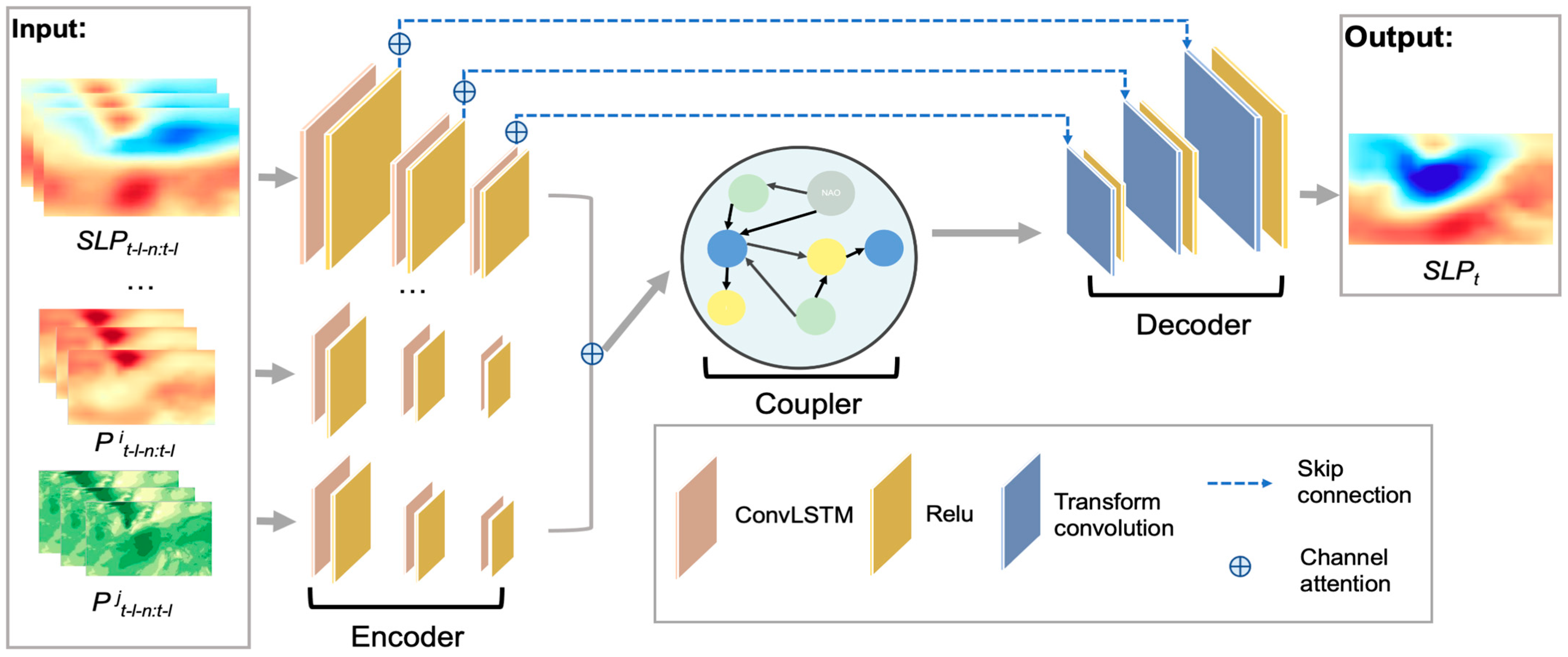
The non-stationarity of the NAO poses a formidable challenge to its forecasting. Here, we address this issue by developing a model with an appropriate structure guided by physical principles. Specifically, we employ graph convolutional networks (GCN) [32] to capture the interactions among meteorological factors, thereby increasing the model’s dynamic simulation capability. We also utilize attention mechanisms to emphasize the more contributory features and supplement the non-stationarity. To this end, we propose the NAO-MCD model for seasonal forecasting of NAO. This model combines a symmetric encoder–decoder structure, attention mechanism, and GCN. As Equation (6), the NAO-MCD can be divided into three parts: an encoder  f e  based on convolutional LSTM (ConvLSTM) [33] networks; a GCN-based coupler  f c ; a decoder  f d  with skip connections [34].
e n c o d e r : L t i = f e P t l n : t l i c o u p l e r : R t = f c L t 1 L t 2 . . L t τ , G . d e c o d e r : S L P t = f d ( R t )
where  t  is forecasted time,  l  is the forecast lead time,  n  is the length of the input sequence, and  P i  indicates the i-th of  τ  predictors.  L i  is the implicit representation of the  P i  after encoding.  G  is the causality between predictors and NAO discovered by the causal discovery algorithms, and R is the result of multivariate coupling. The detailed architecture of NAO-MCD is illustrated in Figure 3. The following sections provide an interpretation of the intentions and detailed implementations of each part of the model.

2.4.1. Encoder

For each predictor  P i , we construct a ConvLSTM-based encoder with the same structure. ConvLSTM is a recurrent neural network, which is designed to learn spatial information of data. ConvLSTM addresses the main drawback of fully connected LSTM by using a convolution operator in the state-to-state and input-to-state transitions. The method determines the future state of a cell in the grid based on the inputs and past states of the local neighbors of that cell. The key equations are shown as follows:
i t = σ W x i X t + W h i H t 1 + W c i C t 1 + b i ,
f t = σ W x f X t + W h f H t 1 + W c f C t 1 + b f ,
C t = f t C t 1 + i t t a n h W x c X t + W h c H t 1 + b c ,
o t = σ W x o X t + W h o H t 1 + W c o C t + b o ,
H t = o t t a n h C t ,
where ∗ represents the convolution operation, and   denotes the Hadamard product. Function  σ  and  tan h  are two kinds of activations.  i t f t , and  o t  are input, forget, and output gate.  X t  is the current input data,  H t 1  is previous hidden output, and  C t  is the cell state.  W  is the weight matrix,  b  is the bias, and both are trainable network parameters. Specifically, each encoder is composed of three layers of ConvLSTM (see Figure 3).
The channel self-attention mechanism is a type of attention mechanism used in deep learning models, which is used to capture the relationship between different channels of a feature map. The mechanism works by computing the attention weights for each channel of the feature map, which is then used to compute a weighted sum of the channels. This allows the model to focus on the most relevant channels for a given task while ignoring irrelevant ones. Depending on the type of channel being fused, we distinguish between two types of channel attention, temporal and parametric, as in Equation (12). First, the temporal channel attention  α t  is applied to obtain the time-weighted sum of the ConvLSTM layers’ encoding output. As a result, information from more valuable lead months will be given greater attention. Second, the parametric channel attention is applied to weight the different variables. The encoded representation of each predictor  L i  is multiplied by the attention weight  a p i . This allows for a more differentiated contribution of different predictors.
α = s o f t m a x ( W 2 t a n h ( W 1 F + b 1 ) + b 2 ) ,
where  α R c n F R c n × f s  is the features,  c n  is the number of channels, and  f s  is the feature size of each channel.  W  and  b  are the transformation matrix and bias, both of which are trained hyperparameters.

2.4.2. Coupler

In some way, the learned causal diagram  G  illustrates the interaction and energy transfer between NAO and the relevant variables, so we construct a two-layer GCN coupler to simulate the information interaction between variables based on  G . GCN is a kind of convolutional neural network that has the ability to directly work with graphs and their structural information. GCN has a multi-layer architecture, with each layer encoding and updating representations of nodes using neighboring features. The l-th layer graph convolution operation is defined as Equation (13):
X l + 1 =   σ D ~ 1 2 A ~ D ~ 1 2 X l W l ,
where  A R N × N  is the adjacency matrix, and  X l R N × M  is the input, with  N  (the same as the number of predictors  P ) nodes in the  G M -dimension encoded feature vector.  A ~ = A + I n , where  I n  is the identity matrix, and  D ~  is the diagonal node degree matrix of  A ~ σ (⋅) denotes the activation function, and  W l  is the trainable transformation matrix parameter. Specially, we convert causal diagram  G  into the form of the undirected graph adjacency matrix  A , which is used to model the interconnection effect between physical variables. In our case, the elements of  A  is defined as follows:
A i , j = 1 , i f   E d g e ( G i , j ) 0 , o t h e r w i s e ,
where  E d g e ( G i , j )  indicates whether an edge exists between the node  i  and  j  in  G , regardless of the edge’s direction.
In practice, the initial input  X  for the coupler is a stacked multivariate encoded feature matrix, and each row is an expanded vector of a physical factor encoded feature  L i . In particular, the vector of SLP is positioned in the last row of the matrix, which corresponds to the last row after coupling, so the vector of the last row of output is the coupled SLP feature to be input into the decoder.

2.4.3. Decoder

We design the decoder symmetrical to the encoder by transforming convolution layers corresponding to the convolution layers in ConvLSTM. Skip connections are also used to directly introduce the original encoded feature into the decoding process. With the cross-layer feature connection module, some important feature information in the higher-level convolution layers can be retained to a greater extent, and more details can be preserved in the multi-scale space. In addition, the skip connection can effectively reduce the gradient disappearance and network degradation, making the training more accessible.

3. Experiments and Evaluations

3.1. Potential Predictors

The key to improving NAO’s forecast skill is understanding the mechanisms governing its variability and identifying the most significant predictors. The earliest proposed mechanisms view NAO as a coupled mode of climate variability between the North Atlantic surface ocean and the overlying atmosphere [35]. As the most commonly calculated source data for the NAOI index, SLP and 500 hPa geopotential height (Z500) were first selected as potential predictors [36]. In addition, the NAOI correlates well with wind speeds in the North Atlantic region, particularly in winter when large-scale circulation has a greater influence on the weather. In addition, the NAO structure can be observed from the first rotating EOF of the monthly average 500 hPa band wind in the Northern Hemisphere [37]. The temporal variability of 10 m wind speed in the central North Atlantic correlates very well with the NAO index, and the annual correlation between the NAO index and the 10 m mean and 98th percentile winds is statistically significant [38]. The strong latitudinal dependence of NAO on the near-surface wind was detected using the GloSea5 seasonal prediction system by Clark et al. [39]. Our pre-experiment demonstrates that the surface wind is more strongly related than the tropospheric 500 hPa wind for the NAOI selected. In addition, to better investigate the sea–air coupling process, we select only the near-surface wind fields V10 (10 m meridional wind) and U10 (10 m zonal wind). Additionally, during the latter part of the twentieth century, the NAO demonstrated greater interannual variability and a positive trend than is expected based on internal atmospheric variability alone. This suggests some external forcing for NAO, such as the ocean or sea ice [40]. In the empirical model constructed by Wang et al. [41] for NAO forecasting, fall sea ice concentration was the strongest predictor of winter NAO. Hall et al. [12] also identified sea ice as a key statistical predictor of winter NAO over the period 1980–2016. Although the relationship between sea ice on NAO may be unsteady [42], drawing on previous experience, we selected the Arctic sea ice extent index as a factor to study the effect of sea ice on NAO. In addition, on seasonal to decadal scales, there is evidence that the ocean plays an active part in determining the NAO’s evolution. While intrinsic atmospheric variability exhibits temporal incoherence, the ocean tends to respond to it with marked persistence of heat content anomalies that provide feedback to the local atmosphere [43]. Accordingly, sea surface latent heat flux (SLHF) are potential predictors to serve as a possible bridge linking the ocean and the atmosphere. Multiple regression of the time series of NAO and SST anomaly centers indicates that parts of the North Atlantic are particularly important for forcing NAO [44]. Therefore, the local SST in the North Atlantic may be an important potential oceanic predictor. Retroaction of anomalous extratropical sea surface temperature (SST) upon the NAO is however under debate and likely depends on the time scale [45]. The impact of ENSO on NAO has been controversially discussed for several decades, which remains uncertain [46]. There is no clear correlation between their monthly and winter indices over the last fifty years, and the relationship may be asymmetric and non-stationary [47]. La Niña events seem to favor positive NAO phases, while El Niño events might not induce systematic remote responses [48]. Thus, we attempt to explore the complex impact of ENSO on NAO using causal discovery algorithms.
According to the above analysis, we selected the potential predictors as described in Table 1, namely the atmospheric variables SLP, Z500, V10, and U10; the oceanic variables SST and SLHF; and the oceanic index variables Niño 3.4 and SeaIceExtent in the non-North Atlantic region.

3.2. Datasets and Pre-Processing

As the observational dataset, the monthly and winter PC-based NAOI from 1899 to 2021 is produced by the Climate Analysis Section of the National Audit of Cardiac Rehabilitation (NCAR). As the source data for the NAOI calculation on the NCAR website, the monthly SLP observations data from 1899 to 2021 are provided by NCAR at 5° resolution. We maintain a consistent calculation method and data source with the PC-based NAOI from the NACR website to ensure that the forecasted NAOs are all observed events. In the datasets for causal discovery, the monthly ocean–atmosphere variables data are obtained from the European Centre for Medium-Range Weather Forecasts (ECMWF) ERA5 [49] global reanalysis product for 1950–2021 with a resolution of 0.25°, and the Niño 3.4 index and sea ice extent index are from NCAR and National Snow and Ice Data Center Data (NSIDC), respectively [50]. In the NAO forecast process, the monthly data for the remaining ocean–atmosphere variables (Z500, V10, U10, SST, SLHF) from 1950 to 2021 are obtained from ERA5 with a resolution of 0.5°, except for the observational data SLP. To account for the limited observational data record, we use transfer learning by pre-training the model on climate simulation data from 1899 to 1949 by the E3SM-1-0 model in Coupled Model Intercomparison Project Phase 6 (CMIP6) [51]. Table 2 details the variable data sets and data types used.
Min–max scaling pre-processing can normalize the dataset and restrict each value to the [0,1] interval, limiting the impact of outliers and facilitating backpropagation. Min–max scaling involves transforming each feature by Equation (15):
x n e w = x x m i n x m a x x m i n .
In the pre-processing, all the data are first normalized, where the grid data are restricted to the North Atlantic region (20° N–80° N, 90° W–40° E). In the causal discovery, the grid data are averaged to one-dimensional time series. Detrending is essential for the non-linearity and non-stationarity of the data [52], which has been widely used in previous climate studies. Thus, we apply detrending and depersonalizing for each time series. Furthermore, all input grid data for NAO-MCD are up-sampled to 5° resolution, so the size of all North Atlantic region grid data is retained at 13 × 27.

3.3. Loss Function

We use a combined loss function for training. According to the different loss combinations, different models are obtained for the ensemble forecast. As shown in Equation (16), the least square deviation L2 loss maintains the smoothness of the prediction results, and the least absolute deviation L1 loss focuses on extreme values. L2 loss has a fast convergence rate, but it leads to a large impact of outliers in training. L1 loss is not overly sensitive to outliers and can better characterize the distribution of normal data, which is more robust. However, it is not conducive to the convergence of the function and the learning of the model, and the model learning speed is slow, so the combination of these two losses can result in faster convergence and good robustness of the model.
L 2 _ L o s s = 1 K Ω K Ω y ^ i , j y i , j 2 L 1 _ L o s s = 1 K Ω K Ω y ^ i , j y i , j , i , j Ω .
where  y ^  is the ground truth and  y  is the forecast result.  K  represents the number of samples,  Ω  represents the number of grid points, and ( i , j ) represents the specific longitude and latitude. Furthermore, Structural Similarity Index (SSIM) is used to focus on predicting exhaustive NAO spatial distributions and reduce the global structural differences between prediction and observation fields. SSIM is a perceptual metric to measure the similarity between two patterns. The main indicators are luminance, contrast, and structure, namely the mean value and standard deviation of a field, and the covariance of the two fields. SSIM is calculated as Equation (17), which ranges from [−1, 1], with larger values representing more similarity. Equation (18) converts the SSIM to the SSIM loss.
S S I M y ^ , y = 2 μ y ^ μ y + C 1 + 2 σ y ^ y + C 2 μ y ^ 2 + μ y 2 + C 1 σ y ^ 2 + σ y 2 + C 2 ,
S S I M _ L o s s = ( 1 S S I M ) 2 ,
where  μ y ^  ( μ y ) represents the average of  y ^  ( y ),  μ y ^  ( μ y ) is the standard deviations of  y ^  ( y ),  σ y ^ y  is the cross-covariance, and  C 1  and  C 2  are constants to avoid the error caused by the denominator being zero. Equation (19) shows how our training loss function is made up of L2 loss, L1 loss, and SSIM loss:
L o s s = β 1 L 2 _ L o s s + β 2 L 1 _ L o s s + β 3 S S I M _ L o s s ,
where  β  is the weighting factor whose exact value will be discussed in the following section.

3.4. Experiment Setting

Ensemble methods have been widely used in NAO forecasts to eliminate noise and thus provide skilled forecasts [53]. The NAO-MCD produces an ensemble forecast of NAO, in which the individual models consist of different input sequence lengths  l  and losses with different weighting parameters  β . It is experimentally demonstrated that the effect of the input sequence length  l  gradually increases from 1 to 5, is flat from 5 to 6, and decreases when it is greater than 7, so we selected the  l  as 5 or 6. Similarly, it is found that the forecast ability of the model is stable at an ensemble size of six. Therefore, we construct the following six ensemble members, as shown in Table 3.
The hyperparameters of the model were determined by fine-tuning through ablation experiments, i.e., fixing other parameters and finding optimal values on the current parameters. The sizes of ConvLSTM kernels are all 3 × 3, which is sufficient for the small-scale input of 13 × 27. The channel sizes of the three ConvLSTM layers are {4, 8, 16} during forward propagation. These incremental numbers of channels can increase the ability of the model to extract complex features in high dimensions by layer. For training, the best batch size is 32, the maximum Epoch is 500, and the learning rate is 0.001. Considering the non-stationary nature of the data, the optimizer is the adaptive moment estimation method (Adam) [54]. The whole monthly data set spans from 1899 to 2021. To ensure that the model is reliably trained, we use the monthly data from 1899 to 2009 as the training data for the model. However, the data in the training set is relatively small for our complex machine learning model, which may lead the model to overlearn in the limited data and fall into overfitting. Overfitting is manifested by an almost infinite decrease in loss during training and an increase in loss on the test set instead, so we divided the data from 2010 to 2014 as the validation set to prevent the model from overfitting with the early stopping method [55]. Early stopping is a regularization technique that stops training once the performance on a validation dataset stops improving. The early stop ensures the generalization ability and makes the model have high forecasting skills on the test set as well. Finally, the model forecasts are validated on a test set from 2015 to 2021. To prevent data leakage at the division junction, the training set has a forecast target that extends up until December 2009. As such, the input to the training set ends in December minus the maximum forecast lead time of 2009. This ensures that the input of the training data is not included in either the training or validation sets.

3.5. Evaluation Metrics

We use root mean square error (RMSE) and SSIM to measure the accuracy of SLP grid data predicted directly by NAO-MCD. The NAO forecast skill is evaluated as the correlation coefficient between the predicted NAOI  I p  and observed NAOI  I o  for each lead time. Correlation coefficient is a very common measure of predictive skill between predictions and observations, especially for indices. The correlation coefficient  r  is defined as follows:
r = i = 1 n I o i I o I p i I p i = 1 n I o i I o 2 i = 1 n I p i I p 2 ,
where  n  is the number of samples, and  I  is the average of  I .

4. Experimental Results and Analysis

To begin with, we show the results of the causal discovery algorithms for the causality of NAO and the associated potential predictors. Then, the optimal set of predictors  P  is selected from the causal diagrams. Next, we evaluate the NAO-MCD from two aspects. First, we compared the forecast skills of NAO-MCD and the state-of-the-art seasonal numerical seasonal forecast models from Copernicus Climate Change Service (C3S) [56] on the test set. Second, we design some comparative experiments to investigate the effectiveness of the NAO-MCD’s model structure. These experiments include an evaluation of the efficacy of causal discovery, an evaluation of the contribution of different predictors, and a comparison with other advanced deep learning models.

4.1. Results of Causal Discovery and Predictor Selection

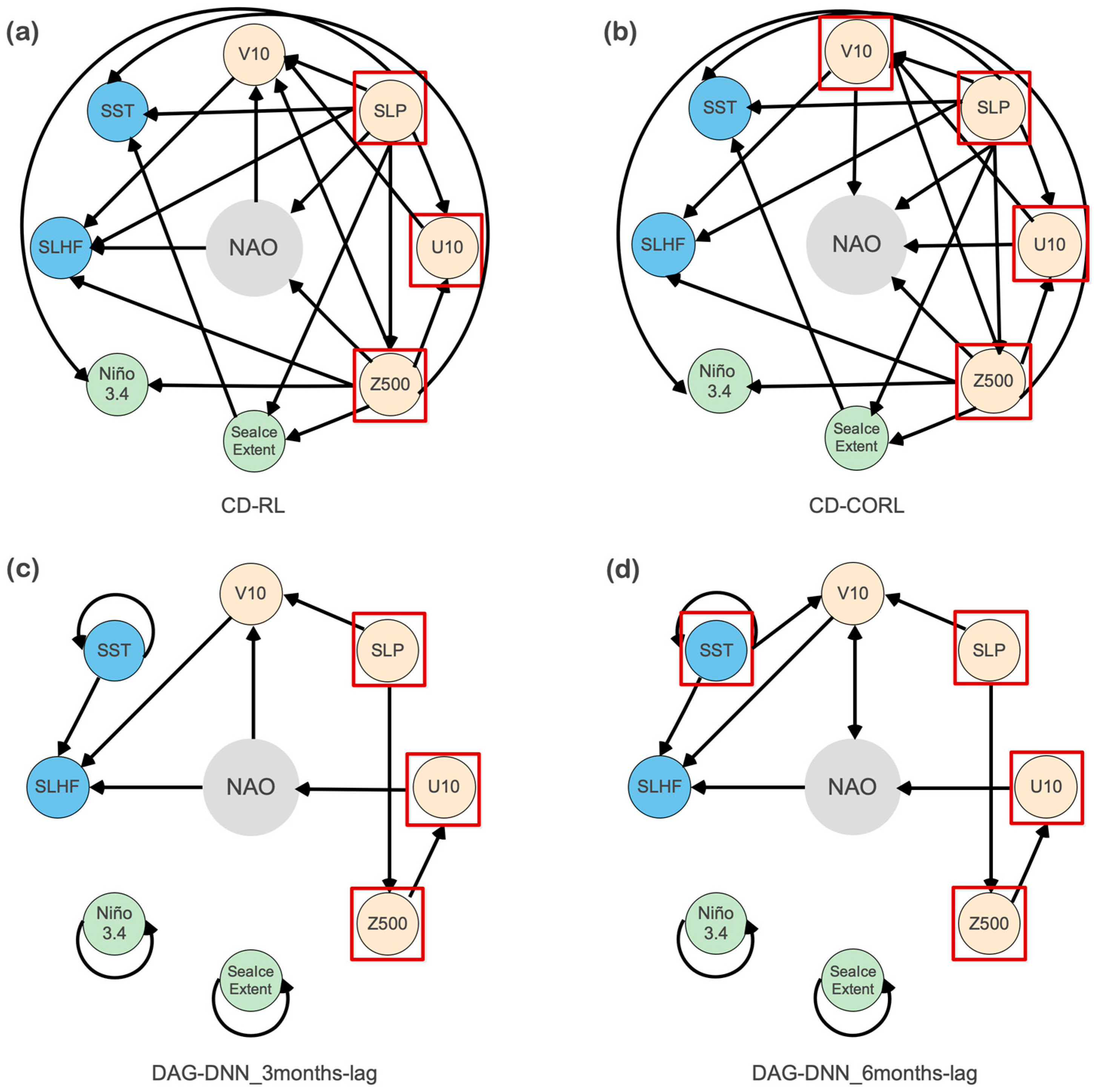
We utilize the causal discovery algorithms CD-RL and CD-CORL to construct DAG-formed causal diagrams that depict the static causality of NAO and potential predictors. In experiments investigating causal discovery in sea ice and atmospheric phenomena, the DAG-GNN has demonstrated its ability to generate sophisticated and meaningful temporal causal representations. Given that we forecast NAO at lead times of 1–6 months, it was imperative to examine temporal causality across sub-seasonal to seasonal timescales with time lags. To achieve this, DAG-GNN generated causal diagrams with fewer edges to facilitate a more detailed examination of stronger time-lagged causality. Specifically, 1–3- and 1–6-month lagged versions of each variable are added to the dataset. Then, DAG-GNN proceeds through the extended dataset to develop 3-month and 6-month lagged temporal circular causal diagrams. The results of causal discovery are shown in Figure 4, where the causality of SLP, Z500, and U10 on NAO is demonstrated in all four causal diagrams. All three algorithms capture the causality between selected atmospheric predictors and NAO, which indicates that NAO is primarily a process of the atmosphere. In addition, in both the 3-month lag and static causal diagrams, SST does not appear to be causally related to NAO, but it appears in the 6-month lag temporal causal diagram. It may indicate that the North Atlantic SST anomaly has a long-term influence on the NAO and provide evidence of the oceanic forcing of NAO. This may be ascribed that surface SST anomalies have a persistent effect on atmosphere-ocean heat fluxes, with substantial thermal coupling between the North Atlantic SST and the atmosphere [57]. However, none of the oceanic index predictors are considered causal to NAO by the algorithms. This may be because the index only represents the phenomenon’s strength, which does not contain spatial information. When Arctic Sea ice extent and El Niño are non-Atlantic, their remote effects on NAO are not easily detected by data-driven approaches.
Finally, optimal predictor set  P = { S S T , Z 500 , U 10 , V 10 , S L P }  is derived from the concatenated set of all predictors determined to be causal for NAO by the casual discovery algorithms. Correspondingly, the input adjacency matrix  A  for the GCN coupler in the NAO-MCD is calculated by the union of all causal diagrams and is defined as follows:
A = 1 1 1 1 1 0 1 1 1 1 0 1 1 1 1 0 1 1 1 1 0 1 1 1 1 .
Furthermore, we perform a correlation analysis between potential predictors and NAO for comparison. The Welch-Satterthwaite equation as Equation (22) is used to calculate the effective degrees of freedom  d f  for the detrended data for the student-t test of the correlation coefficient. According to the Pearson correlation coefficients and p-values of the t-test in Table 4, set  P = { S L P , Z 500 , V 10 , U 10 , S L H F } ,  which has relatively strong correlations significant at the 90% confidence level with NAO, is chosen as the comparative predictors set. The corresponding matrix A input to GCN is an all-one matrix.
d f = s 1 2 n 1 + s 2 2 n 2 s 1 2 n 1 2 n 1 1 + s 2 2 n 2 2 n 2 1 ,
where  d f  is the effective degree of freedom,  s 1  and  s 2  are the sample variances of the two groups, and  n 1  and  n 2  are the sample sizes.

4.2. Analysis of Effective Seasonal NAO Forecast of NAO-MCD

4.2.1. Effect of Ensemble Size

We mainly compare the correlation ( r ) forecast skill of NAO-MCD and C3S for NAO seasonal forecasts. C3S provides a multi-system seasonal forecast service, which is produced by seven seasonal forecast systems. For the test period from 2015 to 2021, only two air–sea coupled systems provide available forecasts, Environment and Climate Change Canada (ECCC) with low resolution and the ECMWF with high resolution. A detailed description of each of them is shown in Table 5.
To begin with, we verify the relationship between the ensemble forecast skill and ensemble size, with ECMWF and ECCC each having 25 and 10 ensemble members. For consistency with deep learning, the monthly average forecast produced by a numerical model initialized on the 1st of that month is regarded as a 1-month lead forecast in this study, which may be regarded as a 0-month lead in meteorology, etc. As seen in Figure 5, ECMWF and ECCC’s monthly NAO forecast skills at a 1-month lead time increase with the number of ensemble members and remain relatively stable after six and three numbers, respectively. We also obtain a regular forecast using NAO-MCD when the ensemble size reaches 3. To facilitate a fair comparison, we use the ensemble mean forecast with six ensemble members of both C3S models and NAO-MCD.

4.2.2. Monthly NAO Forecast

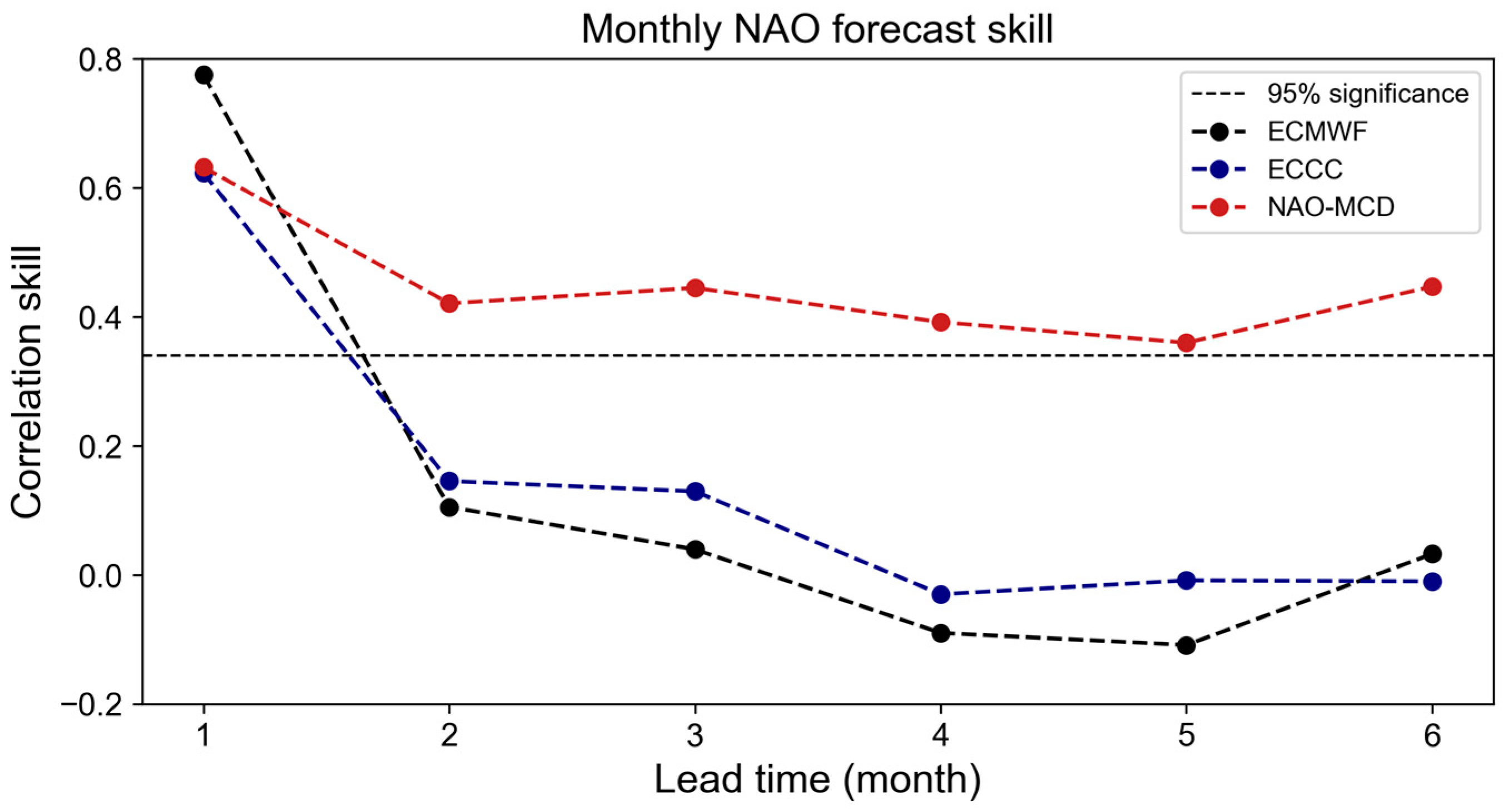
A description of the NAO forecast correlation skill versus lead time of C3S models and NAO-MCD over the 84 test months is shown in Figure 6, demonstrating the excellent ability of NAO-MCD’s long-term forecasting. However, for a 1-month lead monthly NAO forecast, NAO-MCD is inferior to high-resolution models like ECMWF but comparable to low-resolution models like ECCC. This inferiority may be due to NAO-MCD only receiving monthly averages as input, obscuring weather phenomena and initial conditions that determine predictability on short timescales. However, NAO-MCD outperforms the C3S forecast models for lead times exceeding two months. The forecast skills of the C3S models plummet to below 0.2 at a lead time of 2 months and even stay near 0 at a lead time of 3 months and beyond. As a result, C3S is incapable of simulating the NAO development process and forecasting the NAO more than a month in advance. In contrast, NAO-MCD’s forecast skill at 2–6-month lead times is over 0.4, significant at the 95% confidence level, thereby proving ideal for long-term seasonal forecasts. Surprisingly, the forecast capability of NAO-MCD remains strong over time, even rebounding at a 6-month lead time. This rebound is not a coincidence; in our previous study using machine learning methods to predict NAO variability, there was a rebound in prediction accuracy at both the 6-month and 12-month lead times [16]. A possible explanation is that the most salient changes in Atlantic SLP values occur at 6-month and 1-year intervals [58]. These changes can be identified and captured by the machine learning model, resulting in skill vibration. To summarize, the NAO event is mainly an atmospheric process with strong abruptness. The model tends to obtain relatively average results, and the short lead time cannot capture the development of the NAO event as well as numerical models. However, this is also an advantage as there will be no excessive abnormal development, making the prediction results of 2–6 months better than those of traditional numerical models.
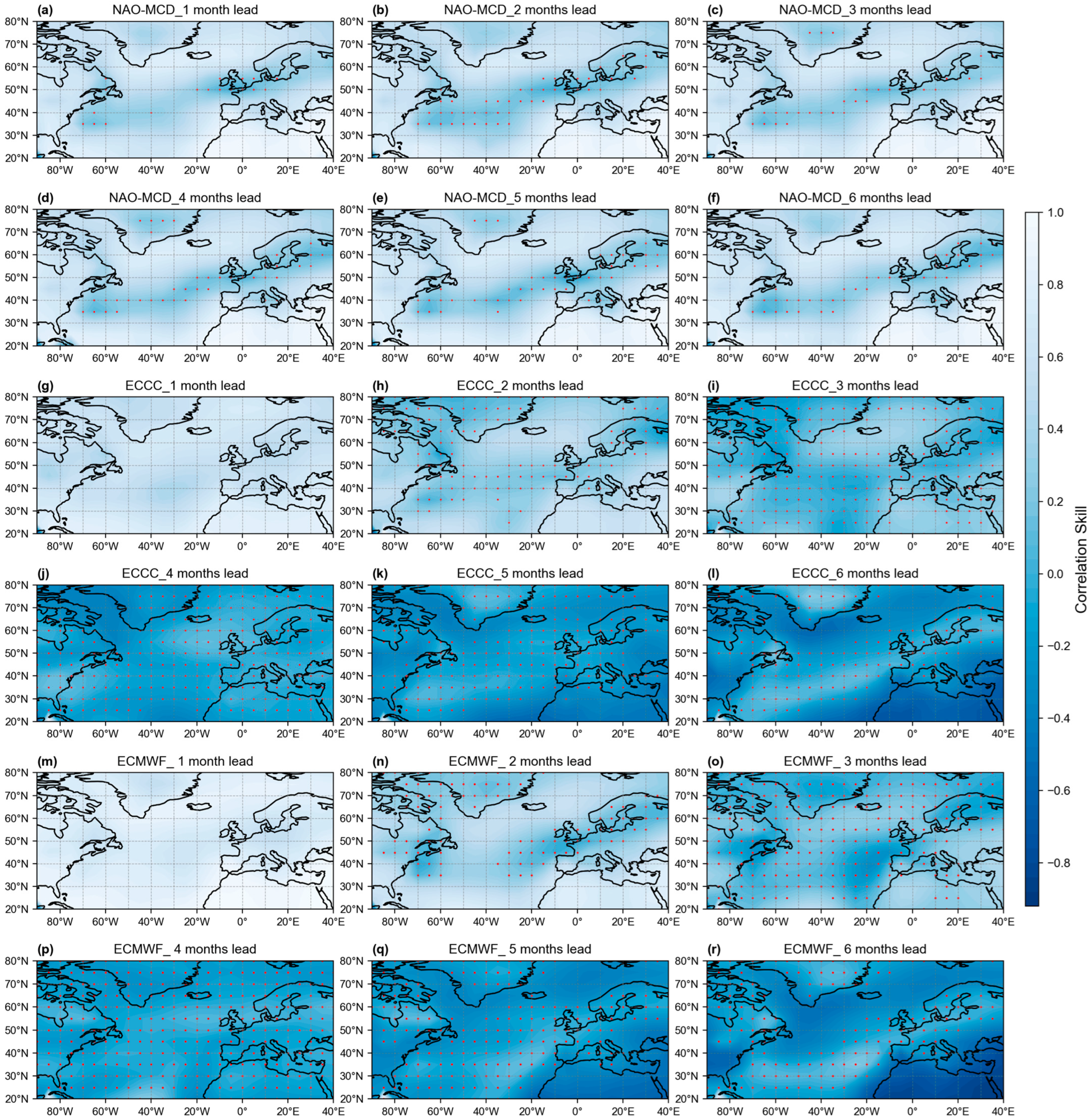
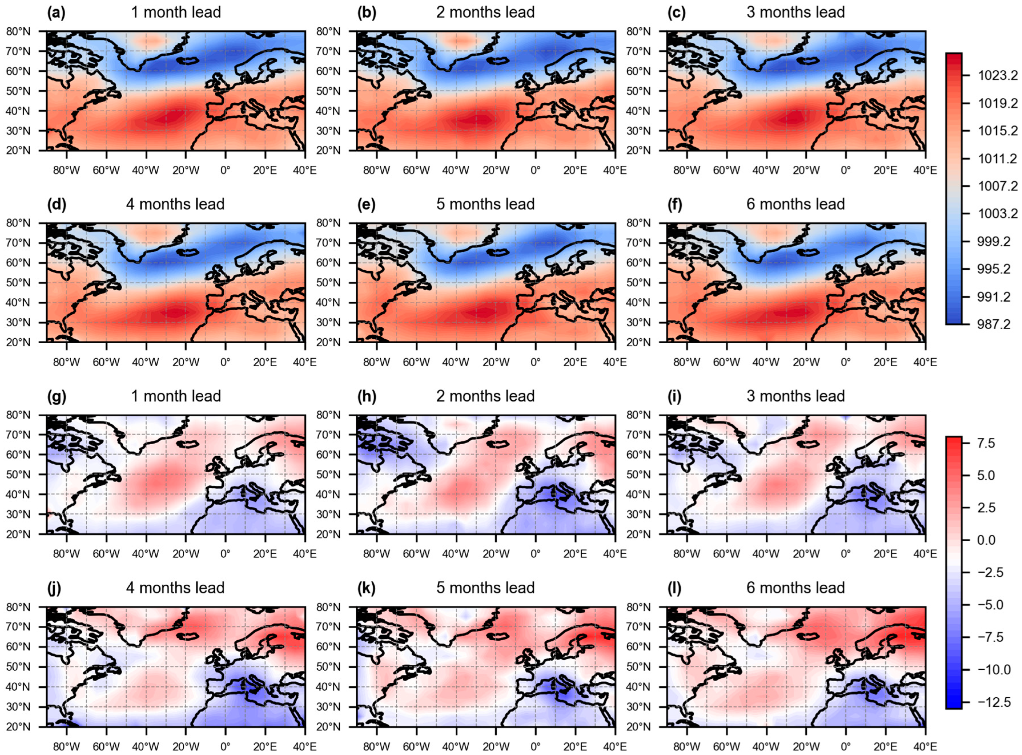
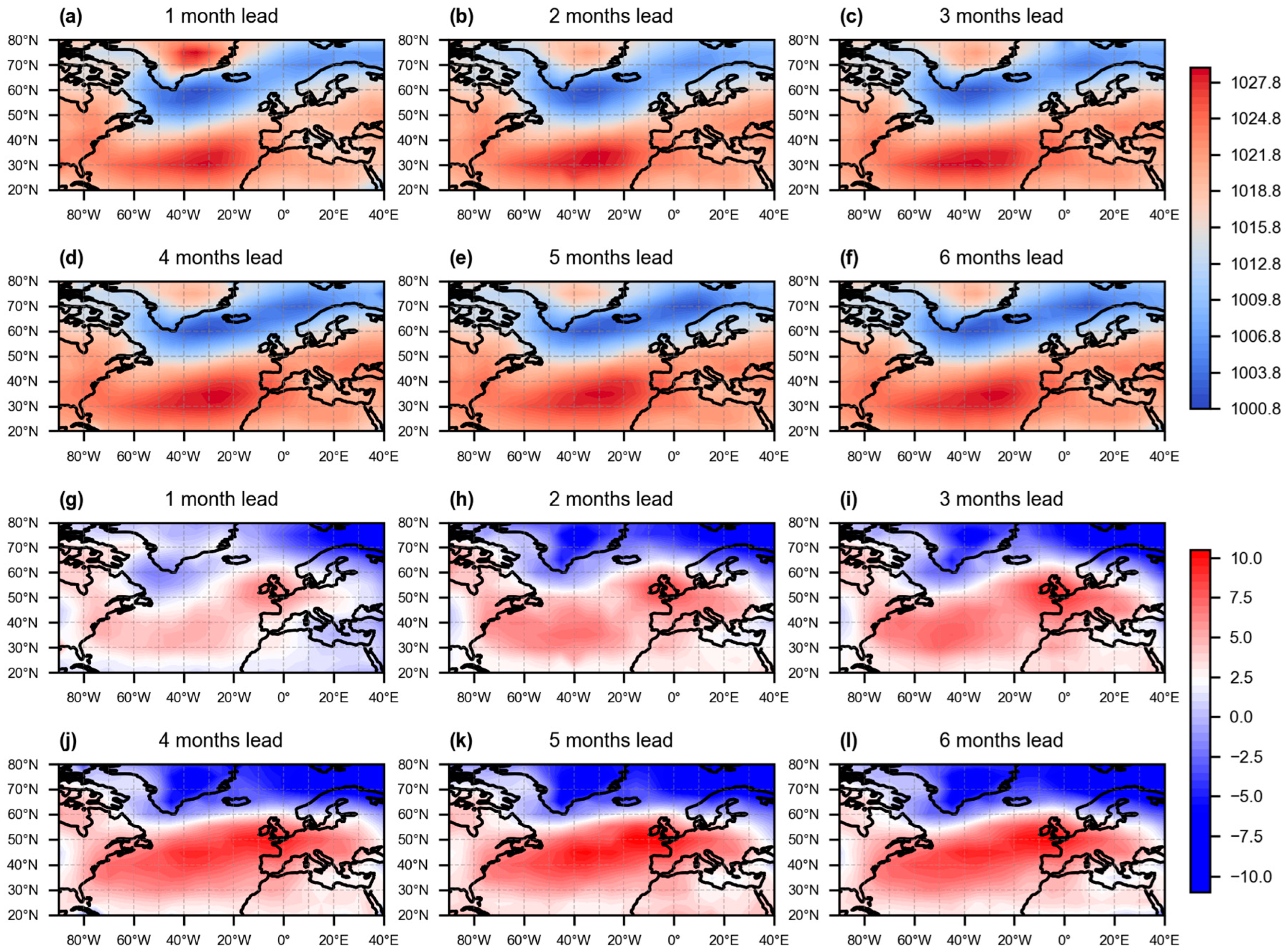
In addition, we evaluate the performed correlation skills between each point of SLP spatial results of C3S and NAO-MCD models’ forecasts at different lead times and observations to better analyze the forecast performance and learned physical mechanisms. Figure 7 shows the correlation skill between ECMWF, ECCC, and NAO-MCD 1–6-month lead time forecasts and observed SLP field spatial grid points. Red dots are the error points where the correlation skill is nonsignificant at the 90% confidence level. For 1-month lead time forecasts, C3S models can predict the spatial structure of each point well, with only some errors in the mid-latitude area in NAO-MCD’s forecasts. As the forecast lead time of NAO-MCD increases, except for the intensification of forecast errors in the 2-month lead forecast, there is no significant development in the mid-latitude forecast errors. However, after the 3-month lead time, errors begin to develop near Greenland Island and disappear by the 6-month lead time. Moreover, the spatial distribution of errors in ECCC and ECMWF’s 2-month lead time forecasts increases significantly, reaching a peak at the 3–4-month lead time and decreasing at the 6-month lead time. Compared with C3S models, it can be seen that NAO-MCD’s forecast error after 2 months of lead time is slight, especially since 3–6 months is much smaller than C3S. The error is similar to the spatial results of C3S’s two-month lead time forecast error, indicating that NAO-MCD may have learned physical mechanisms similar to advanced numerical models. However, this error does not accumulate rapidly like numerical models but remains stable, indicating the superiority of the model for long-term forecasting. In addition, regardless of the distribution and size of errors in the three models, a trend of increasing within the 1–4-month forecast lead time and significantly decreasing at 6 months is shown. Similar trends can be seen in the forecast results for monthly NAOI Figure 6. This indicates that NAO (or SLP) may have a cyclicality of about six months. In particular, it can be seen that there is a significant decrease in errors in the belt area at mid-latitudes and near the Norwegian Sea. In addition, the joint part of model forecast errors, especially the mid-latitude North Atlantic (30° N–50° N, 70° W–0° and 50° N–60° N, 0°–40° E) and Greenland, which are significant in NAO-MCD forecast errors, are likely to be the target observation-sensitive areas for NAO events.
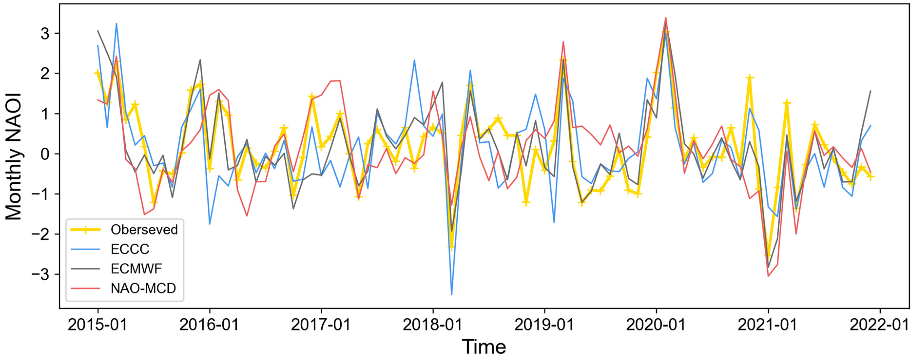
However, the forecast skill measures linear relationships between variables and may be misleading if there are outliers. Next, the forecast performance of the NAO-MCD is assessed in a more detailed visualization of the index values at a 1-month lead time. Figure 8 displays the observed monthly NAOI from 2015 to 2021 and the forecasted results based on the models with a 1-month lead. It appears that the ECMWF has the most stable forecast capability with minor false forecasts, while ECCC and NAO-MCD have more similar forecast results.
Periods, when the absolute value of NAOI exceeds 1, are considered strong NAO events, which are more influential. Thus, we particularly evaluate the models’ forecast skills for extreme NAO events. Table 6 gives the definitions of strong positive NAO++ and strong negative NAO−− and the number of them in the test set. The number of correct forecasts of NAO++ and NAO−− events by the models at a 1-month lead time is shown in the table. It is demonstrated that NAO-MCD has a similar forecast ability to numerical models, with a better judgment of positive events than negative events for extreme NAO.
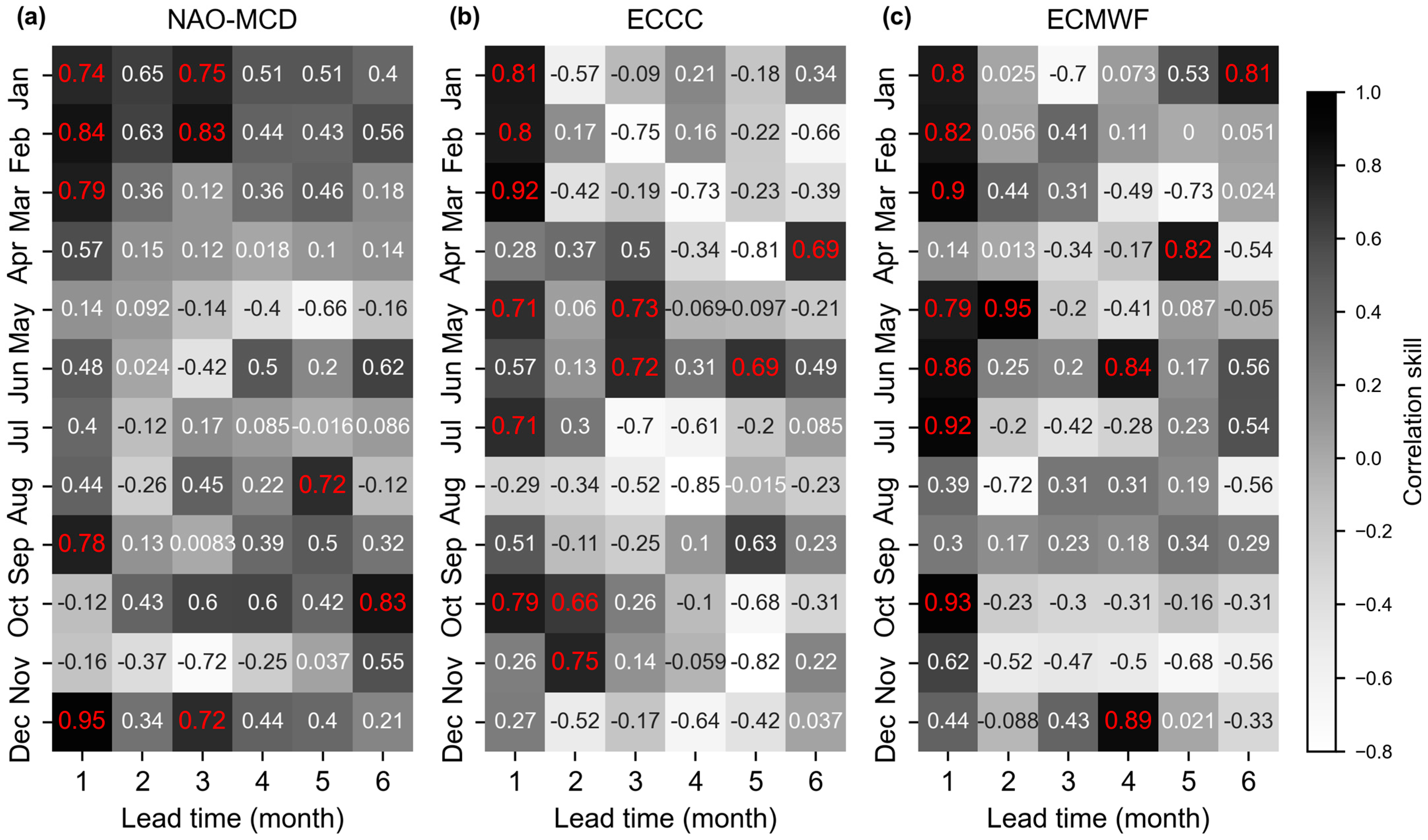
A focus is also placed on the effects of NAO forecasts in different calendar months. Figure 9 shows the model’s forecast skills for each calendar month in the test set. The long-term forecast skills of NAO-MCD for winter (DJFM) NAO are mostly above 0.4, which are far better than that of ECCC and ECMWF. Specifically, NAO-MCD achieves favorable forecasts for December, whereas ECCC and ECMWF produce very high levels of randomness. Next, we analyze the effect of forecasting the specific NAOI for the winter average.

4.2.3. Winter NAO Forecast

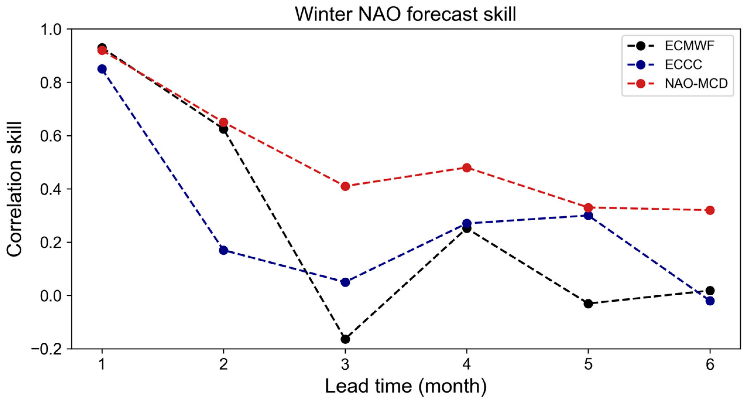
NAO is usually most prominent during winter, causing significant impacts on climate. The winter (DJF) NAOI measures NAO events averaged over the winter time. Figure 10 shows the capability of models to forecast the winter NAO. It can be seen that NAO-MCD has a more stable and superior long-term forecast skill than ECMWF and ECCC.
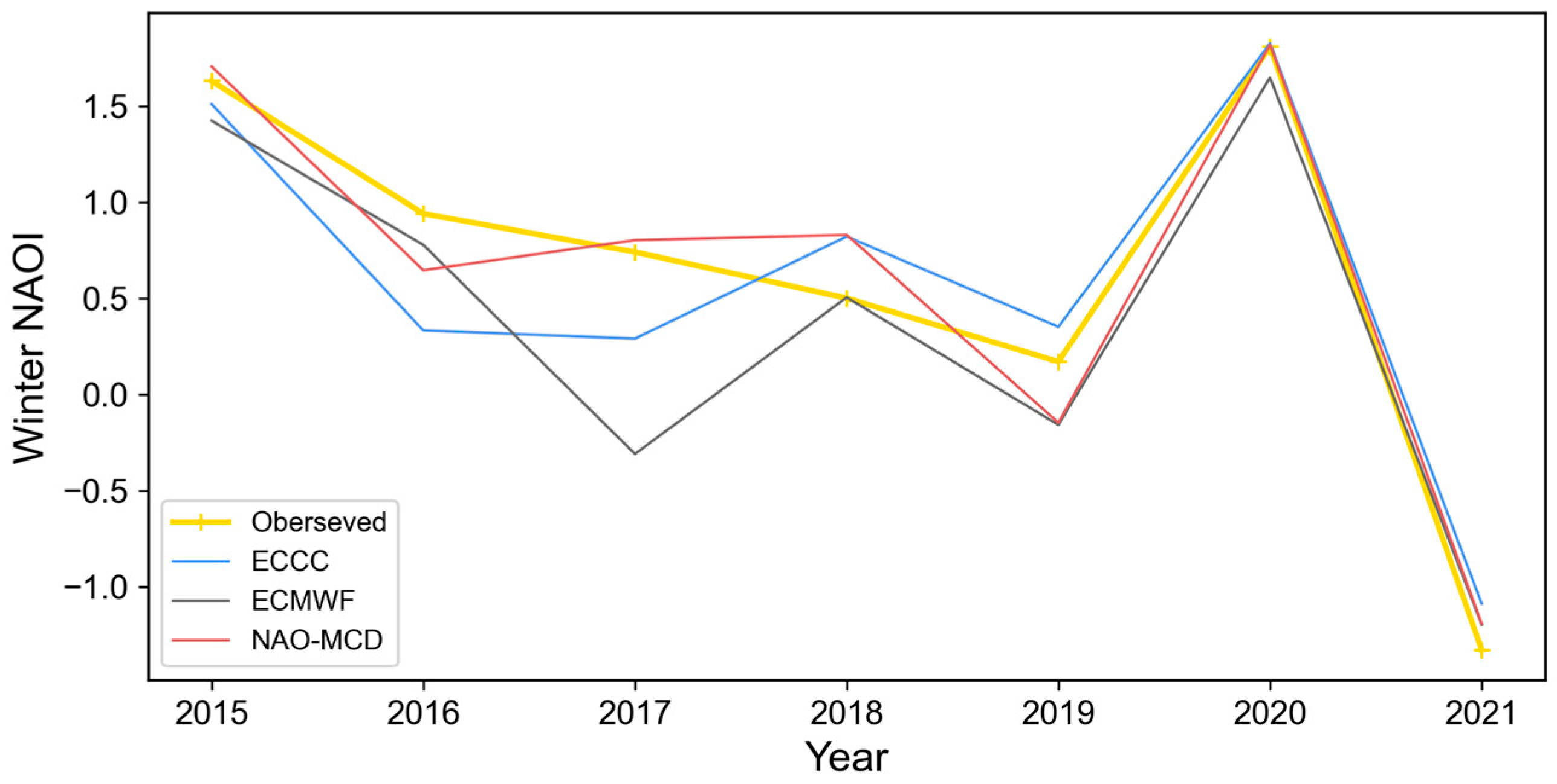
The forecast results for the winter NAOI over the 7 test years with a 1-month lead time are shown in Figure 11. All the models demonstrate reasonable forecast capability for extreme NAO events with relatively larger NAOI, such as in 2015, 2020, and 2021. NAO-MCD has a more robust forecast capability than ECCC, for ECCC inverts the negative and positive phases of NAO events in 2017.
In order to specifically verify the capability of NAO-MCD in forecasting NAO events and analyze the source of prediction errors in spatial structure, we visualize the predicted SLP fields of two NAO++ and NAO−− events. As shown in Figure 12 and Figure 13, they, respectively, represent the strong positive NAO++ in 2020 and the strong negative NAO−− in 2021. It is clear that NAO-MCD is capable of forecasting the bipolar see-saw structure (Icelandic high and Azores low) of the pressure as NAO mode in the long term. However, as the forecast period grows longer, it becomes more difficult for NAO-MCD to simulate the bipolar dual structure, resulting in larger errors. We found that the forecast error of NAO++ mainly comes from the overestimation of low pressure in the Norwegian Sea area, and as the forecast lead time progresses, the error mainly increases towards the western continental area. The forecast error of NAO−− mainly comes from the overestimation of low-latitude high pressure and underestimation of high-latitude low pressure, especially the serious underestimation of Icelandic high pressure after a one-month lead time. However, the forecast error of NAO−− events for a 3–6-month lead time does not obviously develop, which also shows the ability of NAO-MCD to resist disturbance development.

4.3. Effectiveness of the NAO-MCD’s Model Structure

A series of comparison experiments are conducted to verify the usability of the NAO-MCD’s model structure. Rather than evaluating the forecast skill of NAO directly, we focus on the role that the model plays in forecasting the SLP fields. The spatial consistency of the simulated SLP fields and ground truths is measured by SSIM, and the forecast capability for SLP grid values is measured by RMSE. To conduct fair comparisons, the input sequence length  l  for all the comparison experimental models is 6. The parameters of the loss function  β 1 β 2 , and  β 3  are 2, 6, and 7, respectively.

4.3.1. Contributions of Different Predictors to the Forecast Skill

Firstly, to verify the unbiasedness and robustness of the model, we add perturbations to the different parameters of the input to observe the degradation of the model performance. The added perturbation is a Gaussian noise with a standard deviation of 0.05 times the standard deviation of the original data.
Table 7 shows the performance of the model with a 1-month lead time forecast after adding different perturbations. It can be seen that the model has strong stability and the forecasting skill performance only produces a decrease of 0.002 and 0.001 when the perturbations are added to SLP and V10. The perturbations of other factors have very little effect on the model. In addition, the prediction performance of the model decreases by 0.007, RMSE increases by 0.052 hpa, and SSIM decreases by 0.01% after adding perturbations to all factors. These results indicate that the model has good stability in addition to the relatively large contribution of SLP and V10 to the forecast. Further, the analysis of the different contributions of other variables to the forecast results helps to partially understand the impact extent of air–sea variables on NAO. Thus, we design an ablation experiment to remove one predictor from NAO-MCD and assess how this affected forecast skill.
Table 8 shows that the forecast ability for SLP is reduced when each predictor is removed from the model inputs. For PC-Based NAOI forecasting, SLP is undoubtedly the most critical predictor. More specifically, the decrease is most pronounced when the zonal wind (U10) is removed. This demonstrates that the zonal wind is considered to be highly correlated with the NAO mechanism. It has been found that the NAO positive phase is associated with enhanced zonal winds at middle and high latitudes [59]. As a complement to the SLP, which is also a pressure variable, the Z500 has the least impact on forecast ability. Additionally, SST’s influence increases with forecast lead time. This may further indicate that SST has a persistent influence on NAO.

4.3.2. Effectiveness of Causal Discovery and the Coupler

To verify the validity of the causal discovery, we perform a comparison experiment using the correlation-found predictors  P = { S L P , Z 500 , V 10 , U 10 , S L H F } .  The difference between the correlation predictors and the causal predictors is that the former contains SST while the latter contains SLHF. The performance of NAO-MCD with the correlation predictor as inputs is shown in Table 9, which indicates that causality versus correlation is more instructive for forecasting.
The GCN coupler considers each physical variable separately and emphasizes causality-based non-linear interactions between them. To verify the effectiveness of the coupler, we constructed a contrasting NAO-MCD model structure without the coupler, which concatenates each encoder’s results as input to the decoder. The results (Table 9) show that our GCN coupler is a reasonable structure for modeling multivariate interactions, which provides insight into NAO-related dynamical interactions and underlying physical processes.

4.3.3. Comparison with Other Advanced Deep Learning Models

We compared NAO-MCD with other advanced deep learning models, including (1) a convolutional neural network (CNN) and (2) a ConvLSTM network. As the lead time increases, the performance of the models gradually decreases, as in Table 9. The results show the gap between the effectiveness of the spatio-temporal forecast model ConvlSTM and the basic deep learning model CNN. This implies that the complex network structure is more effective in mining the complex dependencies deeply hidden in the evolution of NAO. Overall, NAO-MCD outperforms other models at all lead times, which illustrates the superiority of our model.

5. Discussion and Conclusions

The physical mechanisms and air–sea processes associated underlying the NAO remain uncertain, posing a challenge for traditional models to provide accurate long-term forecasts. This paper provides a data-driven causal discovery perspective to uncover the causality between multiple air–sea variables and NAO changes. The explored causal diagrams reveal that NAO is mainly driven by internal atmospheric dynamics, with the oceanic SST having a lagged effect of approximately 6 months on NAO. Furthermore, we develop an air–sea coupled deep learning model, NAO-MCD, which provides highly accurate seasonal forecasts of NAO. Our experimental results demonstrate that the predictors selected in our causal diagrams are closely related to NAO development and have high physical interpretability. Among these predictors, the zonal wind significantly contributes to our NAO forecasts, while SST exhibits a long-term effect that increases over time.
A further significance of this work lies in posing a challenge to traditional numerical model models. Our models demonstrate the potential of data-driven and machine learning-based approaches to climate model development by providing fast and accurate results. Analysis of the forecast results of the CS3 models and NAO-MCD at 1- to 6-month lead times of monthly and winter NAO shows that the forecast capability of NAO-MCD far exceeds that of numerical models without any long-term forecast skill. The forecasting capability of NAO-MCD at a 1-month lead time is comparable to that of the low-resolution numerical model. The NAO-MCD monthly and winter NAO forecast skill remains around 0.4 at 2–6-month lead times, which is far superior to that of numerical models. In addition, the spatial structure of the errors in NAO-MCD forecasts does not spread to potentially sensitive regions at two-month forecast lead times, as does the numerical model, and spreads to the entire North Atlantic region at 3- to 6-month lead times, losing forecast capability. The good performance may be derived from the fact that deep learning models only learn from inputs and the initial perturbation of climate variables does not evolve over time like numerical models. Inversely, the poor forecasts of the numerical models come mainly from the incomplete dynamical mechanisms involved. It is possible that the forecast skills in the 1-month lead come from the initial condition. For longer-lead forecasts, the dynamic models do not produce a correct response pattern in the NAO. However, the limitations inherent in conventional models can be circumvented through the use of data-driven models that leverage advanced algorithms to discern previously unidentified non-linear physical connections by extracting features autonomously from the data. Additionally, we discovered that NAO may have a six-month cyclicality and mid-latitude North Atlantic (30° N–50° N, 70° W–0° and 50° N–60° N, 0°–40° E) and Greenland may be the observation-sensitive targeted areas.
The study highlights the potential of data-driven methods as a powerful tool for seasonal NAO forecast and air–sea interaction simulation. Despite the significant contributions made by this study, there are several limitations. First, the causal discovery algorithms driven by data can only perform mutual causal analysis on data from the same time period (monthly), and cannot analyze NAO events at specific times, such as a particular season. However, the seasonality of NAO events makes it helpful to conduct separate seasonal analyses and forecasts. Furthermore, our experiments suggest that the causal discovery algorithms may struggle to identify factors with long-term impacts on NAO or those that exhibit teleconnections. Second, although data-driven methods can aid in predicting the future by utilizing past and current information, the quality of predictions is heavily influenced by the quality and quantity of data available. As monthly forecasting is conducted in this study, the earliest observation data for SLP dates back to 1899, with only slightly over 1300 monthly data points available. The limited data may lead to overfitting issues during model training. Third, deep learning, as a black-box method, lacks the ability to provide reasonable explanations regarding the learned features and their physical implications.
Moving forward, several avenues of research may be pursued to overcome these limitations. One promising direction is to explore alternative causal discovery algorithms that are capable of analyzing NAO events at specific times and better account for seasonal variability. Future studies may also explore the use of additional remotely related but important variables such as equatorial Middle and East Pacific ENSO events, tropical SST anomalies, and snowpack to improve forecast accuracy. To address the issue of limited data, efforts could be made to incorporate data from a wider range of sources. For one example, using data from high-quality assimilated model simulations to learn the physics contained in the model. It is also important to develop methods that can handle missing data, as this may improve the robustness of the models. To better understand the physical implications of the features learned by deep learning models, future research may explore methods for interpreting and visualizing the internal representations of these models. Such efforts could provide valuable insights into the underlying physical mechanisms and help validate the models’ predictions. Overall, while data-driven approaches have limitations, there are several promising avenues for future research that may help overcome these limitations and further our understanding of NAO dynamics and their impacts.

Author Contributions

Conceptualization, B.M. and X.J.; methodology, X.J.; software, X.J. and B.Q.; data curation, X.J.; writing—original draft preparation, X.J.; writing—review and editing, S.Y., Y.C. and B.M.; supervision, S.Y.; project administration, B.M.; All authors have read and agreed to the published version of the manuscript.

Funding

This research was funded by the Meteorological Joint Funds of the National Natural Science Foundation of China (grant number U2142211), the Key Project Fund of Shanghai 2020 “Science and Technology Innovation Action Plan” for Social Development (grant number 20dz1200702), the National Key Research and Development Program of China (grant number 2020YFA0608000), the National Natural Science Foundation of China (grant number 42075141, 41875057, 41730960), and the first batch of Model Interdisciplinary Joint Research Projects of Tongji University in 2021 (grant number YB-21-202110).

Institutional Review Board Statement

Not applicable.

Informed Consent Statement

Not applicable.

Data Availability Statement

Data used in this paper are available in publicly accessible repositories: the PC-based NAOI data are provided by the Climate Analysis Section in NCAR at https://climatedataguide.ucar.edu/climate-data/hurrell-north-atlantic-oscillation-nao-index-pc-based, accessed 20 December 2022; the monthly SLP data are available in the Computational and Information Systems Laboratory of NCAR at https://rda.ucar.edu/datasets/ds010.1, accessed on 20 December 2022, doi:10.5065/Z88P-AW38; the ERA5 data are available in the Climate Data Store (CDS) at https://cds.climate.copernicus.eu, accessed on 20 December 2022, doi:10.24381/cds.6860a57; the CMIP6 data are available in the CDS at https://cds.climate.copernicus.eu, accessed on 20 December 2022, doi:10.24381/cds.c866074c; the CS3 forecast data are available in the CDS at https://cds.climate.copernicus.eu, accessed on 20 December 2022, doi:10.24381/cds.68dd14c3.

Acknowledgments

Thanks to Adam Phillips from the Climate and Global Dynamics Division of the NCAR, for his technical guidance on the detailed calculation methodology and pre-processing details of the PC-based NAO index.

Conflicts of Interest

The authors declare no conflict of interest.

References

  1. Hurrell, J.W.; Kushnir, Y.; Visbeck, M. The North Atlantic Oscillation. Science 2001, 291, 603–605. [Google Scholar] [CrossRef]
  2. Hurrell, J.W. Decadal Trends in the North Atlantic Oscillation: Regional Temperatures and Precipitation. Science 1995, 269, 676–679. [Google Scholar] [CrossRef] [PubMed]
  3. Hurrell, J.W.; Van Loon, H. Decadal Variations in Climate Associated with the North Atlantic Oscillation. In Climatic Change at High Elevation Sites; Diaz, H.F., Beniston, M., Bradley, R.S., Eds.; Springer: Dordrecht, The Netherlands, 1997; pp. 69–94. [Google Scholar] [CrossRef]
  4. Donat, M.; Peterson, T.; Brunet, M.; King, A.; Almazroui, M.; Kolli, R.; Boucherf, D.; Al-Mulla, A.; Nour, A.; Aly, A.; et al. Changes in Extreme Temperature and Precipitation in the Arab Region: Long-Term Trends and Variability Related to ENSO and NAO. Int. J. Climatol. 2014, 34. [Google Scholar] [CrossRef]
  5. Rousi, E.; Rust, H.W.; Ulbrich, U.; Anagnostopoulou, C. Implications of Winter NAO Flavors on Present and Future European Climate. Climate 2020, 8, 13. [Google Scholar] [CrossRef]
  6. Athanasiadis, P.J.; Bellucci, A.; Scaife, A.A.; Hermanson, L.; Materia, S.; Sanna, A.; Borrelli, A.; MacLachlan, C.; Gualdi, S. A Multisystem View of Wintertime NAO Seasonal Predictions. J. Clim. 2017, 30, 1461–1475. [Google Scholar] [CrossRef]
  7. Weisheimer, A.; Schaller, N.; O’Reilly, C.; MacLeod, D.A.; Palmer, T. Atmospheric Seasonal Forecasts of the Twentieth Century: Multi-Decadal Variability in Predictive Skill of the Winter North Atlantic Oscillation (NAO) and Their Potential Value for Extreme Event Attribution: Atmospheric Seasonal Forecasts of the Twentieth Century. Q. J. R. Meteorol. Soc. 2017, 143, 917–926. [Google Scholar] [CrossRef] [PubMed]
  8. Kent, C.; Scaife, A.A.; Dunstone, N. What Potential for Improving Sub-Seasonal Predictions of the Winter NAO? Atmos. Sci. Lett. 2023, 24, e1146. [Google Scholar] [CrossRef]
  9. Richter, J.H.; Glanville, A.A.; Edwards, J.; Kauffman, B.; Davis, N.A.; Jaye, A.; Kim, H.; Pedatella, N.M.; Sun, L.; Berner, J.; et al. Subseasonal Earth System Prediction with CESM2. Weather Forecast. 2022, 37, 797–815. [Google Scholar] [CrossRef]
  10. Lin, H. Predictability and Prediction of the North Atlantic Oscillation. In Proceedings of the ECMWF Seminar on Predictability in the European and Atlantic Regions, Reading, UK, 6–9 September 2010. [Google Scholar]
  11. Tao, L.-J.; Gao, C.; Zhang, R.-H. Model Parameter-Related Optimal Perturbations and Their Contributions to El Niño Prediction Errors. Clim. Dyn. 2019, 52, 1425–1441. [Google Scholar] [CrossRef]
  12. Hall, R.J.; Scaife, A.A.; Hanna, E.; Jones, J.M.; Erdélyi, R. Simple Statistical Probabilistic Forecasts of the Winter NAO. Weather Forecast. 2017, 32, 1585–1601. [Google Scholar] [CrossRef]
  13. Strommen, K.; Palmer, T.N. Signal and Noise in Regime Systems: A Hypothesis on the Predictability of the North Atlantic Oscillation. Q. J. R. Meteorol. Soc. 2019, 145, 147–163. [Google Scholar] [CrossRef]
  14. Yuan, S.; Luo, X.; Mu, B.; Li, J.; Dai, G. Prediction of North Atlantic Oscillation Index with Convolutional LSTM Based on Ensemble Empirical Mode Decomposition. Atmosphere 2019, 10, 252. [Google Scholar] [CrossRef]
  15. Cuesta, J.E.; Hunt, J.K.; Schull, J. Weekly Climate Indices: Generation and Prediction. 2019. Stanford Research Series. Available online: https://medium.com/comet-ml/stanford-research-series-weekly-climate-indices-generation-and-prediction-8e548babb3a7 (accessed on 10 January 2023).
  16. Mu, B.; Li, J.; Yuan, S.; Luo, X. The NAO Variability Prediction and Forecasting with Multiple Time Scales Driven by ENSO Using Machine Learning Approaches. Comput. Intell. Neurosci. 2022, 2022, e6141966. [Google Scholar] [CrossRef] [PubMed]
  17. Siddique, T.; Mahmud, M.S.; Keesee, A.M.; Ngwira, C.M.; Connor, H. A Survey of Uncertainty Quantification in Machine Learning for Space Weather Prediction. Geosciences 2022, 12, 27. [Google Scholar] [CrossRef]
  18. Ebert-Uphoff, I.; Deng, Y. Causal Discovery for Climate Research Using Graphical Models. J. Clim. 2012, 25, 5648–5665. [Google Scholar] [CrossRef]
  19. Song, H.; Wang, J.; Tian, J.; Huang, J.; Zhang, Z. Spatio-Temporal Climate Data Causality Analytics—An Analysis of ENSO’s Global Impacts. In Proceedings of the 8th International Workshop on Climate Informatics (CI2018), Boulder, CO, USA, 19–21 September 2018. [Google Scholar]
  20. Huang, Y.; Kleindessner, M.; Munishkin, A.; Varshney, D.; Guo, P.; Wang, J. Benchmarking of Data-Driven Causality Discovery Approaches in the Interactions of Arctic Sea Ice and Atmosphere. Front. Big Data 2021, 4, 72. [Google Scholar] [CrossRef]
  21. He, S.; Yang, S.; Chen, D. Accurate Attribution and Seasonal Prediction of Climatic Anomalies Using Causal Inference Theory. J. Clim. 2022, 35, 4111–4124. [Google Scholar] [CrossRef]
  22. He, S.; Yang, S.; Chen, D. Inferring Causal Structures to Model and Predict ENSO and Its Effect on Asian Summer Monsoon. In Proceedings of the EGU General Assembly 2023, Vienna, Austria, 24–28 April 2023. EGU23-102. [Google Scholar] [CrossRef]
  23. Jones, P.D.; Osborn, T.J.; Briffa, K.R. Pressure-Based Measures of the North Atlantic Oscillation (NAO): A Comparison and an Assessment of Changes in the Strength of the NAO and in Its Influence on Surface Climate Parameters. In The North Atlantic Oscillation: Climatic Significance and Environmental Impact; American Geophysical Union (AGU): Washington, DC, USA, 2003; pp. 51–62. [Google Scholar] [CrossRef]
  24. Hurrell, J.W.; Deser, C. North Atlantic Climate Variability: The Role of the North Atlantic Oscillation. J. Mar. Syst. 2010, 79, 231–244. [Google Scholar] [CrossRef]
  25. Wunsch, C. The Interpretation of Short Climate Records, with Comments on the North Atlantic and Southern Oscillations. Bull. Am. Meteorol. Soc. 1999, 80, 245–256. [Google Scholar] [CrossRef]
  26. Chevillon, G. Direct Multi-Step Estimation and Forecasting. J. Econ. Surv. 2007, 21, 746–785. [Google Scholar] [CrossRef]
  27. Pearl, J. Models, Reasoning and Inference; Cambridge University Press: Cambridge, UK, 2000; Volume 19. [Google Scholar]
  28. Zhu, S.; Ng, I.; Chen, Z. Causal Discovery with Reinforcement Learning. arXiv 2019, arXiv:1906.04477. [Google Scholar]
  29. Wang, X.; Du, Y.; Zhu, S.; Ke, L.; Chen, Z.; Hao, J.; Wang, J. Ordering-Based Causal Discovery with Reinforcement Learning. arXiv 2021, arXiv:2105.06631. [Google Scholar]
  30. Yu, Y.; Chen, J.; Gao, T.; Yu, M. DAG-GNN: DAG Structure Learning with Graph Neural Networks. In International Conference on Machine Learning; PMLR: San Diego, CA, USA, 2019; pp. 7154–7163. [Google Scholar]
  31. Hochreiter, S.; Schmidhuber, J. Long Short-Term Memory. Neural Comput. 1997, 9, 1735–1780. [Google Scholar] [CrossRef]
  32. Kipf, T.N.; Welling, M. Semi-Supervised Classification with Graph Convolutional Networks. arXiv 2016, arXiv:1609.02907. [Google Scholar]
  33. Shi, X.; Chen, Z.; Wang, H.; Yeung, D.-Y.; Wong, W.-K.; Woo, W. Convolutional LSTM Network: A Machine Learning Approach for Precipitation Nowcasting. In Proceedings of the International Conference on Neural Information Processing Systems, Montreal, QC, Canada, 7–12 December 2015; pp. 802–810. [Google Scholar]
  34. Ronneberger, O.; Fischer, P.; Brox, T. U-Net: Convolutional Networks for Biomedical Image Segmentation. In Proceedings of the Medical Image Computing and Computer-Assisted Intervention–MICCAI 2015: 18th International Conference, Munich, Germany, 5–9 October 2015; Part III 18. Springer: Berlin/Heidelberg, Germany, 2015; pp. 234–241. [Google Scholar]
  35. Bjerknes, J. Atlantic Air-Sea Interaction. In Advances in Geophysics; Landsberg, H.E., Van Mieghem, J., Eds.; Elsevier: Amsterdam, The Netherlands, 1964; Volume 10, pp. 1–82. [Google Scholar]
  36. Thompson, D.W.J.; Wallace, J.M. The Arctic Oscillation Signature in the Wintertime Geopotential Height and Temperature Fields. Geophys. Res. Lett. 1998, 25, 1297–1300. [Google Scholar] [CrossRef]
  37. Woollings, T.; Hannachi, A.; Hoskins, B.; Turner, A. A Regime View of the North Atlantic Oscillation and Its Response to Anthropogenic Forcing. J. Clim. 2010, 23, 1291–1307. [Google Scholar] [CrossRef]
  38. Laurila, T.K.; Sinclair, V.A.; Gregow, H. Climatology, Variability, and Trends in near-Surface Wind Speeds over the North Atlantic and Europe during 1979–2018 Based on ERA5. Int. J. Climatol. 2021, 41, 2253–2278. [Google Scholar] [CrossRef]
  39. Clark, R.T.; Bett, P.E.; Thornton, H.E.; Scaife, A.A. Skilful Seasonal Predictions for the European Energy Industry. Environ. Res. Lett. 2017, 12, 024002. [Google Scholar] [CrossRef]
  40. Feldstein, S.B. The Timescale, Power Spectra, and Climate Noise Properties of Teleconnection Patterns. J. Clim. 2000, 13, 4430–4440. [Google Scholar] [CrossRef]
  41. Wang, L.; Ting, M.; Kushner, P.J. A Robust Empirical Seasonal Prediction of Winter NAO and Surface Climate. Sci. Rep. 2017, 7, 279. [Google Scholar] [CrossRef]
  42. Kolstad, E.W.; Screen, J.A. Nonstationary Relationship Between Autumn Arctic Sea Ice and the Winter North Atlantic Oscillation. Geophys. Res. Lett. 2019, 46, 7583–7591. [Google Scholar] [CrossRef]
  43. Cassou, C. Euro-Atlantic Regimes and Their Teleconnections. In Proceedings of the ECMWF Seminar on Predictability in the European and Atlantic Regions, Reading, UK, 6–9 September 2010; Volume 6, pp. 1–14. [Google Scholar]
  44. Rodwell, M.J.; Rowell, D.P.; Folland, C.K. Oceanic Forcing of the Wintertime North Atlantic Oscillation and European Climate. Nature 1999, 398, 320–323. [Google Scholar] [CrossRef]
  45. Zhang, W.; Jiang, F. Subseasonal Variation in the Winter ENSO-NAO Relationship and the Modulation of Tropical North Atlantic SST Variability. Climate 2023, 11, 47. [Google Scholar] [CrossRef]
  46. Feng, P.-N.; Lin, H.; Derome, J.; Merlis, T.M. Forecast Skill of the NAO in the Subseasonal-to-Seasonal Prediction Models. J. Clim. 2021, 34, 4757–4769. [Google Scholar] [CrossRef]
  47. Hurrell, J.W.; Kushnir, Y.; Ottersen, G.; Visbeck, M. An Overview of the North Atlantic Oscillation. In The North Atlantic Oscillation: Climatic Significance and Environmental Impact; American Geophysical Union (AGU): Washington, DC, USA, 2003; pp. 1–35. [Google Scholar] [CrossRef]
  48. Bell, C.J.; Gray, L.J.; Charlton-Perez, A.J.; Joshi, M.M.; Scaife, A.A. Stratospheric Communication of El Niño Teleconnections to European Winter. J. Clim. 2009, 22, 4083–4096. [Google Scholar] [CrossRef]
  49. Hersbach, H.; Bell, B.; Berrisford, P.; Hirahara, S.; Horányi, A.; Muñoz-Sabater, J.; Nicolas, J.; Peubey, C.; Radu, R.; Schepers, D.; et al. The ERA5 Global Reanalysis. Q. J. R. Meteorol. Soc. 2020, 146, 1999–2049. [Google Scholar] [CrossRef]
  50. Fetterer, F.; Knowles, K.; Meier, W.N.; Savoie, M.; Windnagel, A.K. Sea Ice Index, Version 3. 2017. Distributed by National Snow and Ice Data Center. Available online: https://doi.org/10.7265/N5K072F8 (accessed on 15 November 2022).
  51. Eyring, V.; Bony, S.; Meehl, G.A.; Senior, C.A.; Stevens, B.; Stouffer, R.J.; Taylor, K.E. Overview of the Coupled Model Intercomparison Project Phase 6 (CMIP6) Experimental Design and Organization. Geosci. Model Dev. 2016, 9, 1937–1958. [Google Scholar] [CrossRef]
  52. Wu, Z.; Huang, N.E.; Long, S.R.; Peng, C.-K. On the Trend, Detrending, and Variability of Nonlinear and Nonstationary Time Series. Proc. Natl. Acad. Sci. USA 2007, 104, 14889–14894. [Google Scholar] [CrossRef]
  53. Scaife, A.A.; Arribas, A.; Blockley, E.; Brookshaw, A.; Clark, R.T.; Dunstone, N.; Eade, R.; Fereday, D.; Folland, C.K.; Gordon, M.; et al. Skillful Long-Range Prediction of European and North American Winters. Geophys. Res. Lett. 2014, 41, 2514–2519. [Google Scholar] [CrossRef]
  54. Kingma, D.P.; Ba, J. Adam: A Method for Stochastic Optimization. arXiv 2017, arXiv:1412.6980. [Google Scholar] [CrossRef]
  55. Prechelt, L. Early Stopping—But When? In Neural Networks: Tricks of the Trade, 2nd ed.; Montavon, G., Orr, G.B., Müller, K.-R., Eds.; Lecture Notes in Computer Science; Springer: Berlin/Heidelberg, Germany, 2012; pp. 53–67. [Google Scholar] [CrossRef]
  56. Thépaut, J.-N.; Dee, D.; Engelen, R.; Pinty, B. The Copernicus Programme and Its Climate Change Service. In Proceedings of the IGARSS 2018—2018 IEEE International Geoscience and Remote Sensing Symposium, Valencia, Spain, 22–27 July 2018; Institute of Electrical and Electronics Engineers: Piscataway, NJ, USA, 2018; pp. 1591–1593. [Google Scholar] [CrossRef]
  57. Bhatt, U.; Alexander, M.; Battisti, D.; Houghton, D.; Keller, L. Atmosphere-Ocean Interaction in the North Atlantic: Near-Surface Climate Variability. J. Clim. 1998, 11, 1615–1632. [Google Scholar] [CrossRef]
  58. Osińska, M.; Jędrasik, J. Atlantic Oscillation Indices in Meridional Distribution. Theor. Appl. Climatol. 2020, 141, 1367–1382. [Google Scholar] [CrossRef]
  59. Woollings, T.; Franzke, C.; Hodson, D.L.R.; Dong, B.; Barnes, E.A.; Raible, C.C.; Pinto, J.G. Contrasting Interannual and Multidecadal NAO Variability. Clim. Dyn. 2015, 45, 539–556. [Google Scholar] [CrossRef]
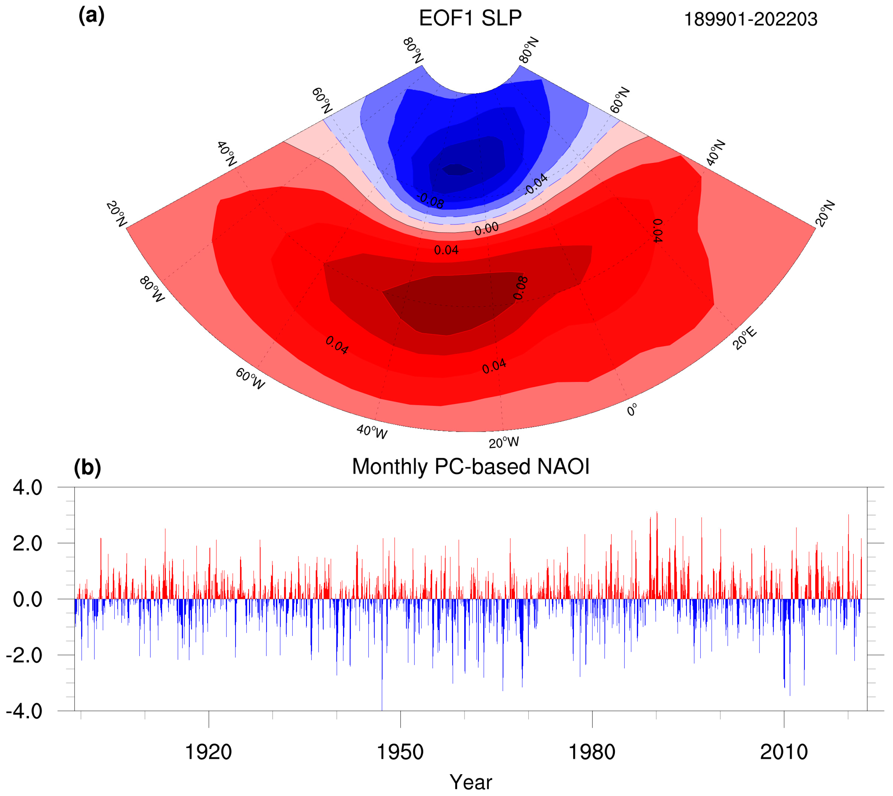
Figure 1. Monthly principal component (PC)-based NAO index (NAOI) and its corresponding first empirical orthogonal function (EOF) model: (a) the leading EOF mode of the monthly sea-level pressure (SLP) anomaly in the North Atlantic (20° N–80° N, 90° W–40° E), which shows a north–south NAO dipole pattern; (b) normalized monthly NAOI from 1899 to 2022 ranges from −4 to +4. The NAOI greater than zero is shown by the red bar, and those less than zero are shown by the blue bar.
Atmosphere 14 00792 g001
Figure 2. Description of the NAO forecast procedure, which consists of two steps of predictors selection and NAOI forecast.
Atmosphere 14 00792 g002
Figure 3. The architecture of NAO-MCD: a multivariate air–sea coupled model for NAO forecast combined with causal discovery. NAO-MCD consists of an encoder, coupler, and decoder. The input is the historical sequence of predictors  P  and the output is SLP of the forecasted time.
Atmosphere 14 00792 g003
Figure 4. Causal diagrams of NAO and potential predictors built by the causal discovery algorithms: (a,b) are the static acyclic causal diagrams DAGs constructed by the CD-RL and CD-CORL algorithms. (c,d) are the temporal circular causal diagrams constructed by DAG-GNN with 3-month and 6-month lag, respectively. The arrows in the diagrams indicate the causality from cause to effect, and the red boxes indicate the predictors that are regarded as the direct or indirect causes of NAO.
Atmosphere 14 00792 g004
Figure 5. The relationship between models’ ensemble forecast skill and ensemble size at a 1-month lead time.
Atmosphere 14 00792 g005
Figure 6. Modes’ monthly NAO forecast skill at 1–6-month lead times. The horizontal line indicates the t-test 95% significance level of the correlations.
Atmosphere 14 00792 g006
Figure 7. Maps of the correlation skills between SLP field grid points predicted by the models 1–6 months in advance and observations: (af) are forecasts by NAO-MCD; (gl) are forecasts by ECMWF and (mr) are forecasts by ECCC. The points in red are forecast tips that are not statistically significant at the 90% confidence level.
Atmosphere 14 00792 g007
Figure 8. Monthly NAOI forecast results from 2015 to 2021 at a 1-month lead time.
Atmosphere 14 00792 g008
Figure 9. Heat map of the model’s correlation skills with NAO forecasts for different calendar months at 1–6-month lead times. Correlation skills above 90% confidence level for non-noise data are marked in red font.
Atmosphere 14 00792 g009
Figure 10. Modes’ winter NAO forecast skill at 1–6-month lead times.
Atmosphere 14 00792 g010
Figure 11. Winter NAOI forecast results from 2015 to 2021 at a 1-month lead time.
Atmosphere 14 00792 g011
Figure 12. Forecasted SLP fields of the strong positive winter NAO++ in 2020: (af) the forecast result; (gl) the forecast error.
Atmosphere 14 00792 g012
Figure 13. Forecasted SLP fields of the strong negative winter NAO−− in 2021 (af) the forecast result; (gl) the forecast error.
Atmosphere 14 00792 g013
Table 1. Potential predictor variables for NAO seasonal predictions.
VariableDescriptionUnit
SLPSea-level pressurehPa
Z500500 hPa geopotential heightm
V1010 m meridional windm·s−1
U1010 m zonal windm·s−1
SSTSea surface temperatureK
SLHFSea surface latent heat fluxJ·m−2
Niño 3.4Niño 3.4 ENSO index-
SeaIceExtentArctic sea ice extent index-
Note: The yellow shade covers the atmospheric variables, the blue shade covers the oceanic variables, and the green shade covers the non-Atlantic oceanic index variables.
Table 2. The detailed dataset descriptions.
VariableTime RangeData SourceData Type
SLP1899–2021NCARObservation
Z5001899–1949
1950–2021
CMIP6
Era5
Model simulation
Reanalysis
V101899–1949
1950–2021
CMIP6
Era5
Model simulation
Reanalysis
U101899–1949
1950–2021
CMIP6
Era5
Model simulation
Reanalysis
SST1899–1949
1950–2021
CMIP6
Era5
Model simulation
Reanalysis
SLHF1899–1949
1950–2021
CMIP6
Era5
Model simulation
Reanalysis
Niño 3.41950–2021NSIDCObservation
SeaIceExtent1950–2021NCARObservation
Table 3. Parameter setting for NAO-MCD ensemble members.
Member
Number
  β   l
  β 1   β 2   β 3
12675
23675
32775
42676
53676
62776
Table 4. Pearson correlation coefficient between NAO and potential predictors. The bold values in the table are the top five Pearson correlation coefficients and the p-values that are statistically significant at the 90% confidence level.
SLPZ500V10U10SSTSLHFNiño 3.4SeaIce
Extent
correlation
coefficient
0.110.110.350.220.0670.120.0350.081
p-value0.00680.00861.3 × 10−152.2 × 10−60.0130.00890.2510.188
Table 5. Description of the available forecast systems in C3S.
Forecast System NameForecast System VersionForecast Initial ConditionModel Resolution
(Model Top)
Available
Ensemble Size
ECMWFSEAS51st of monthTCo319 (~0.36° lat-long)/91 levels in vertical, to 0.01 hPa25
ECCCCanCM4i1st of monthT63 (~2.8° lat-long)/35 levels in vertical, to 1 hPa10
Table 6. The definition of strong NAO events and models’ forecast effects at a 1-month lead time of strong NAO events.
PhaseIndex ValuesNumber in the Test SetNumber of Correct Forecasts
ECMWFECCCNAO-MCD
NAO−−Strong negativeNAOI < −1.09434
NAO++Strong positiveNAOI > 1.0151099
Table 7. Model performance with one predictor added to the perturbation at 1-month lead time.
Perturbed PredictorForecast SkillRSME (hPa)SSIM (%)
-0.5894.06379.674
SLP0.5874.08778.642
Z5000.5894.07279.567
V100.5884.07579.034
U100.5894.06779.568
SST0.5894.07079.535
All0.5824.11578.622
Table 8. Model performance with one predictor removed.
Removed PredictorRSME (hPa)/SSIM (%)
1-Month Lead3-Month Lead6-Month Lead
-4.06/79.674.18/78.124.26/77.15
Z5004.18/78.044.25/76.804.39/76.02
V104.31/77.094.35/75.834.42/75.11
U104.39/76.804.39/75.494.62/75.21
SST4.22/78.604.37/76.054.47/74.47
Table 9. Performance comparison with other models and NAO-MCD with different structures.
ModelRSME (hPa)/SSIM (%)
1-Month Lead3-Month Lead6-Month Lead
CNN5.36/66.236.47/63.127.26/59.15
ConvLSTM4.64/70.254.95/64.775.39/63.89
NAO-MCD with
correlation predictors
4.24/77.734.52/76.134.87/75.02
NAO-MCD without
coupler
4.35/76.794.52/75.724.74/74.35
NAO-MCD4.18/78.044.25/76.804.39/76.02
Disclaimer/Publisher’s Note: The statements, opinions and data contained in all publications are solely those of the individual author(s) and contributor(s) and not of MDPI and/or the editor(s). MDPI and/or the editor(s) disclaim responsibility for any injury to people or property resulting from any ideas, methods, instructions or products referred to in the content.