On the Correlations between Particulate Matter: Comparison between Annual/Monthly Concentrations and PM₁₀/PM_2.5

Abstract

Annual concentration is a key element to assess the air quality of an area for long-time exposure effects. Nonetheless, obtaining annual concentrations from sensors is costly since it needs to have a year of measurements for each required pollutant. To overcome this issue, several strategies are studied to assess annual particulate matter concentration from monthly data, with their pros and cons depending on the risk acceptance and measurement campaign costs. When applied on a French dataset, the error spans from 12–14% with one month of measurement to 4–6% for six months of measurement for PM₁₀ and PM_2.5, respectively. A relationship between the mean relative error and 95th percentile relative error is provided with an R² of 0.99. The relationship between PM₁₀ and PM_2.5 was also investigated and improved compared to previous work by considering the seasonality and influence on emission reaching a mean relative error of 12%. Thus, this study provides tools for urban planners, engineers, researchers, and public authorities for improved monitoring of annual air pollution at a lower cost for particulate matter.

1. Introduction

Air quality is a major concern in European countries, especially in urban areas where high emissions can be observed. Among the numerous air pollutants monitored, particulate matter (PM) was considered the highest priority according to the World Health Organization [1] due to its harmful effects on human health. Studies have shown that PM can have several health impacts such as preterm birth [2], neurodevelopmental disorders [3,4] or short-term health effects [5,6], whereas long-term exposure to these pollutants can significantly increase cardiovascular incident probability and respiratory diseases [7], with the smaller particles being the most harmful [8]. As an example of a health-related impact, around 400,000 people prematurely died in 2016 from PM_2.5 exposure over the European continent [9].

Particulate matters (PM) are complex airborne pollutants composed of a mixture of extremely small particles and other compounds such as metals, organic chemicals, or dust particles [7]. They can come from natural sources (e.g., forest fires) but they are mainly emitted from anthropogenic sources [10]. PMs are generally classified depending on their aerodynamic diameter: the coarse PM having an aerodynamic diameter of 10 µm or less (PM₁₀) and the fine PM having an aerodynamic diameter of 2.5 µm or less (PM_2.5) [11]. According to the WHO, the PM₁₀ are more likely to be produced by mechanical processes (construction activities, dust re-suspension, etc.), whereas PM_2.5 are more likely coming from combustion sources (wood combustion, biomass fuel combustion, etc.) [1]. Thus, according to the WHO, the ratios of PM₁₀ and PM_2.5 must vary subsequently depending on the meteorology, the local geography, and the specific sources of particulate matter. For this work, both PM₁₀ and PM_2.5 were considered but without distinction from their sources.

The European Union (EU) and the World Health Organization (WHO) have issued critical and target values that should not be exceeded in order to protect people from the hazardous effects of PM on human health [12,13]. To compare with these values, air pollution can be assessed using both numerical methods [14,15,16,17,18] and on-site monitoring [19,20].

Numerical modeling can be a powerful tool which can be used to assess pollutant dispersion for complex situations such as noise-barrier configurations [21,22,23] or high-rise buildings [24,25] using computational fluid dynamics or artificial intelligence [26,27], with recent studies dealing with how to compute mean annual concentrations from numerical results [28,29]. Beside this, on-site monitoring has the advantage of giving the actual air pollutant concentrations at the monitoring point. However, year-round measurement data should be gathered to calculate mean annual concentration, which is a significant constraint in terms of time and cost.

A recent study has shown the possibility of assessing annual NO₂ concentrations based on monthly concentration using a methodology based on quadratic functions, thus allowing reducing the necessary monitoring time and, consequently, the costs [30].

Since particulate matter concentrations follow the same logic of seasonality [31,32], the aim of the present study is to check if such methodology can also be implemented for PM₁₀ and PM_2.5 annual concentration assessment. This methodology would be to determine the annual concentrations by using a shorter time period, accounting for seasonality and other variations that may occur over the course of a year, and determine easy-to-use regressions that will improve results for measurement campaigns that cannot afford to have year-round monitoring stations at the same location. Particularly, it is to assess several strategies to compute annual particulate matter concentration from monthly data, with their pros and cons depending on the risk acceptance and measurement campaign costs, and also to find if there is any correlation between PM₁₀ and PM_2.5 concentration evolution. This could help countries and environmental agencies to reduce the cost of assessing annual air quality and thus improving the knowledge of pollutant exposure of dwellers, especially for countries with weak sensors or modeling coverage [33].

The data used in this study are presented in Section 2. The results are then presented in Section 3, with the evolution of PM concentration in France and the methodologies to compute annual concentrations from monthly data and to compute PM_2.5 concentrations from PM₁₀ concentrations. A discussion is provided in Section 4.

2. Materials and Methods

2.1. Study Location

This work was performed at a national scale retrieving PM₁₀ and PM_2.5 concentrations monitored in a large number of regions in France. The location of these regions is presented in Figure 1, and includes, from North to South, Haut-de-France, Normandie, Grand-Est, Ile-de-France, Pays de la Loire, Bourgogne–Franche-Comté, Nouvelle Aquitaine, and Provence-Alpes-Côte d’Azur. A representative view of the variety of locations from France could be covered by these regions as they are located at several latitude and longitude. One of the most critical parts to selecting the regions was also related to the data availability.

2.2. Data Availability

Data were obtained through the open access database provided by the French air quality monitoring authorities known in France as the AASQA acronym (Association Agréée de Surveillance de la Qualité de l’Air), which means “Approved Air Quality Monitoring Associations. The data collected are PM₁₀ and PM_2.5 monthly mean concentrations, mainly observed over a nine-year period from 2011 to 2019. A summary of the available data, corresponding to a total of around 28,000 monthly mean concentrations and 230 different stations, is given in

Table 1. Summary of the available data.

Region	PM10			PM2.5
	Data Availability	Number of Monthly Data	Relative Percentage of the Total Dataset	Data Availability	Number of Monthly Data	Relative Percentage of the Total Dataset
Hauts-de-France	2011–2019	3888	15%	2011–2019	1836	20%
Ile-de-France	2011–2019	3240	13%	2011–2019	1512	24%
Grand-Est	2011–2019	4536	18%	2011–2019	1836	24%
Pays de la Loire	2011–2019	2060	8%	2011–2019	750	10%
Bourgogne–Franche-Comté	2011–2019	1404	6%	2011–2019	1080	14%
Provence-Alpes-Côte d’Azur	2011–2019	3456	14%	2015–2019	490	7%
Nouvelle Aquitaine	2012–2019	3648	15%	-	-	-
Normandie	2011–2019	2808	11%	-	-	-

. Only the data where the full year was available have been retained.

2.3. Data Range

Considering the whole dataset, the monthly mean concentrations range from 24 to 76 µg/m³ and from 1 to 47 µg/m³ for PM₁₀ and PM_2.5, respectively, whereas annual mean concentrations range from 30 to 55 µg/m³ and from 5 to 33 µg/m³. These concentrations correspond to different types of stations (also called “influence”) which include background (66%), industrial (10%), and traffic (24%) stations, as well as different types of areas, including rural (14%), suburban (18%), and urban (68%) areas for PM₁₀. The PM_2.5 station types and influences are not known except for the one where both PM₁₀ and PM_2.5 data exist. There are 25,040 monthly concentrations for the PM₁₀ and 7506 for PM_2.5.

2.4. Statistical Performance Measures

In order to compare the different ways to assess annual PM concentrations from monthly PM concentrations, three statistical performance parameters were considered including (1) the coefficient of determination, (2) the relative error over a given dataset, and (3) the mean relative error over multiple datasets.

$$R^2=1-\frac{{\sum }_{i=1}^n{\left(C_i-\widehat{C_i}\right)}^2}{{\sum }_{i=1}^n{\left(C_i-\overline{C_i}\right)}^2}$$

(1)

where $R^2$ is the coefficient of determination, $n$ is the number of data, $C_i$ is the concentration value, $\widehat{C_i}$ is the predicted corresponding value, and $\overline{C_i}$ is the averaged concentration.

$$R{E}_i={{\displaystyle \sum }}_{j=1}^{n_i}\frac{\left|p_{ij}-d_{ij}\right|}{\left|\overline{d_i}\right|}$$

(2)

where $R{E}_i$ is the relative error for the dataset $i$, $n_i$ is the number of data in the dataset $i$, $p_{ij}$ is the predicted value, $d_{ij}$ is the actual data value, and $\overline{d_i}$ is the averaged actual data value.

$$MRE=\frac{1}{n}{{\displaystyle \sum }}_{i=1}^{n}R{E}_i$$

(3)

where $MRE$ is the mean relative error, $n$ is the number of datasets considered, and $R{E}_i$ is the relative error for the dataset $i$.

In the following, the 95th percentile relative error (P₉₅RE) is the percentile 95 value from the RE_i.

2.5. Months Clustering Based on the Concentration Estimation

A clustering was performed using MetaboAnalyst package on R (version 3.6.3). The clustering was performed by combining the heatmap and the hierarchical ascendent clustering, with distance measure with Euclidean and clustering algorithms using ward.D. The combination of heatmap and clustering was performed to evaluate whether a monthly concentration was higher or lower than the annual concentration using the following equation:

$$Variation=\frac{concentratio{n}_{month}-concentratio{n}_{annual}}{concentratio{n}_{annual}}$$

(4)

3. Results

3.1. PM₁₀ and PM_2.5 Mean Annual Concentration Trends in France

Figure 2A shows the evolution of the PM₁₀ and PM_2.5 mean annual concentration in France between 2011 and 2019. According to these two boxplots, the mean annual concentrations are globally decreasing in France since 2011 for both PM₁₀ and PM_2.5. However, the most significant decrease was observed between 2011 and 2015. After 2015, the mean annual concentrations appear to be steady, even if the mean value averaged over all the stations (red line) is still decreasing. Indeed, considering a linear regression, the regression slope is about −1.3 (respectively, −0.4) between 2011 and 2015 (respectively, 2016 and 2019) for PM₁₀ and about −1.2 (respectively, −0.6) for the same periods for PM_2.5. Thus, there is a slope variation by a factor of 3.25 and 2 for PM₁₀ and PM_2.5, respectively. Please note that these observations are only from the box plots, since no specific statistical tests were performed.

Figure 2 gives additional information by distinguishing the mean annual concentrations by the influence of the station for both PM₁₀ and PM_2.5. According to Figure 2B, a decrease in PM₁₀ concentrations is observed for whatever the influence considered (i.e., background, industrial, and traffic stations), but the higher decrease is observed for traffic stations, nonetheless.

It is the same observation for PM_2.5 concentration, according to Figure 2C, for both background and traffic stations. No comparison can be made between PM₁₀ and PM_2.5 concentration evolution for industrial stations since there is not this kind of station for PM_2.5 available.

As a first approach, the annual PM₁₀ concentrations were plotted as a function of the monthly PM₁₀ concentrations considering the whole dataset (including all years, all regions, all types of stations, and all types of areas). The corresponding results, along with a linear regression line, are presented in Figure 3A. Although the annual concentration appears to be linearly correlated with the monthly concentration, the scatterplot is widely dispersed around the regression line, leading to a low coefficient of determination ($R^2=0.57$). Additionally, considering the obtained line to assess annual concentration from monthly concentration can lead to over or underestimation that can reach 100%.

3.2. Assessment of Annual Concentrations Based on Monthly Data

To improve the results, the same process has been applied considering all months of given years of data. As an example, the results obtained for the year 2019 are presented in Figure 3B. According to this figure, the linear regression is improved when considering the given years of data: $R^2$ = 0.78 is obtained for 2019. The slopes and intercepts of the two linear regressions presented in Figure 3 are of the same order of magnitude, but slightly different, confirming that using all years or each year independently led to different results. The over and underestimation are also lowered but can still reach 50%.

The same methodology used for PM₁₀ has been conducted on PM_2.5. As for PM₁₀, it appears that interpolating the annual PM_2.5 concentration as a function of monthly PM_2.5 concentration with a linear regression led to poor results when considering the whole data, but also each year separately.

As seen previously, the solution considering the whole dataset is not satisfying. To improve the results, the same methodology as in [30] was used. First, a check of whether there are seasonal trends on the variation of the particle matter concentration is performed.

Two main groups can be seen from the clustering given in Figure 4A,B, a group containing the winter months could be distinguished with monthly concentrations higher than the annual concentration on average and the rest of the year with monthly concentrations lower than the annual concentrations on average.

• For PM₁₀ there are 594 samples representing 28.23% of the data belonging to group 1. It is composed mainly of 4 months making up around 90% of the group with February (27%), January (23%), March (25%), and December (16%);
• For PM_2.5 there are 204 samples representing 22.47% of the data belonging to group 1. It is composed mainly of 3 months making up 85% of the group with January (32%), February (30%), and March (26%).

The difference between the seasons could be explained by the more diverse source of particulate matter in winter from heating or cold starting vehicles.

According to Figure 4C, the results obtained using linear regressions considering monthly concentrations against annual ones show that, when using only one month of measurements, the worst months to evaluate the annual concentration are in winter (MRE = 0.15 in winter vs. MRE = 0.11 the rest of the year for PM₁₀ and MRE = 0.17 in winter, vs. MRE = 0.13 the rest of the year for PM_2.5). This is probably related to the fact that the mid-months represent half of the annual concentration, whereas winter only represents a third/quarter and thus are more representative of the annual concentration. Another factor might be that the additional particulate matter from heating may vary between years depending on the climate condition of the winter.

3.3. Assessment of Annual Concentrations Based on Monthly Data by Years

These previous predictions were made using all years. However, as discussed in Section 3.2, considering each year separately improved the results. Thus, it is possible to improve the results by considering each year independently. Indeed, each year could follow a different trend, for example a warmer winter leading to less heating.

When comparing this approach with the previous one, as seen in Figure 5, the MRE is lower for PM₁₀ for every month with an absolute reduction of −0.033 on the MRE corresponding to a relative reduction of 27% on the MRE on average. As for PM₁₀, the prediction of PM_2.5 for annual concentration using monthly data is improved when considering each year independently. The MRE is reduced by −0.050 in absolute and 35% in relative on average.

However, there are two major limits with this method of considering each year independently. First, several sensors are necessary in the area that monitors the concentration throughout the year with enough variety to make a regression. This issue is not a big deal when the country is well covered in sensors as is the case for France. Second, waiting for the end of the year to perform the correlation seems to be inconsistent with engineering issues.

3.4. Assessment of Annual Concentrations Based on a Group of Months

In France, a popular way to evaluate the annual concentration is to measure one month in summer and one month in winter to have a better representativeness of the seasonal variation during the year. Several months can be monitored throughout the year to improve the predictions on the mean annual concentration. But it lacks quantitative information on the gains in accuracy of several months’ measurements compared with one-month measurements. To solve this issue, the mean concentration of several groups of months evenly spaced were studied. For instance, if using two months, the mean of the concentrations between January (1st month) and July (1 + 6 = 7th month) will be computed; with 4 months, the average between January (1st), April (4th), July (7th), and October (10th) will be computed; etc.

Figure 6 shows a comparison of the MRE for both PM₁₀ and PM_2.5 between the use of a linear regression on the average and directly using the average concentration value of the months (equivalent to a linear regression of bias 0 of and intercept of 1).

As expected, the more months, the better the results. This result leads to two key points:

• The slope is stronger from one month to three months than from three months to six months, meaning that the gain in error is maximized up to a period of 3 months for both PM₁₀ and PM_2.5.
• The linear regression improves the results, especially when the number of months used is low. When reaching 3 months, the difference between the linear regression and averaging becomes less than 10%.

As an additional result of the study, an easy way to improve the 2-month results, and, also easy to implement, is to consider and use the observation made on the different types of months that exist: the best results are obtained when using two months that do not contain the winter type of month (i.e., April/October and May/November). Thus, most likely, if a winter month is considered and represents half of the data when averaging the concentrations, it over represents the season. To solve that, weighting the winter-type months (December, January, February, and March) by 1/4 and the rest of the months by 3/4 improves the results as well as the stability of the predictions, as can be seen in Figure 7.

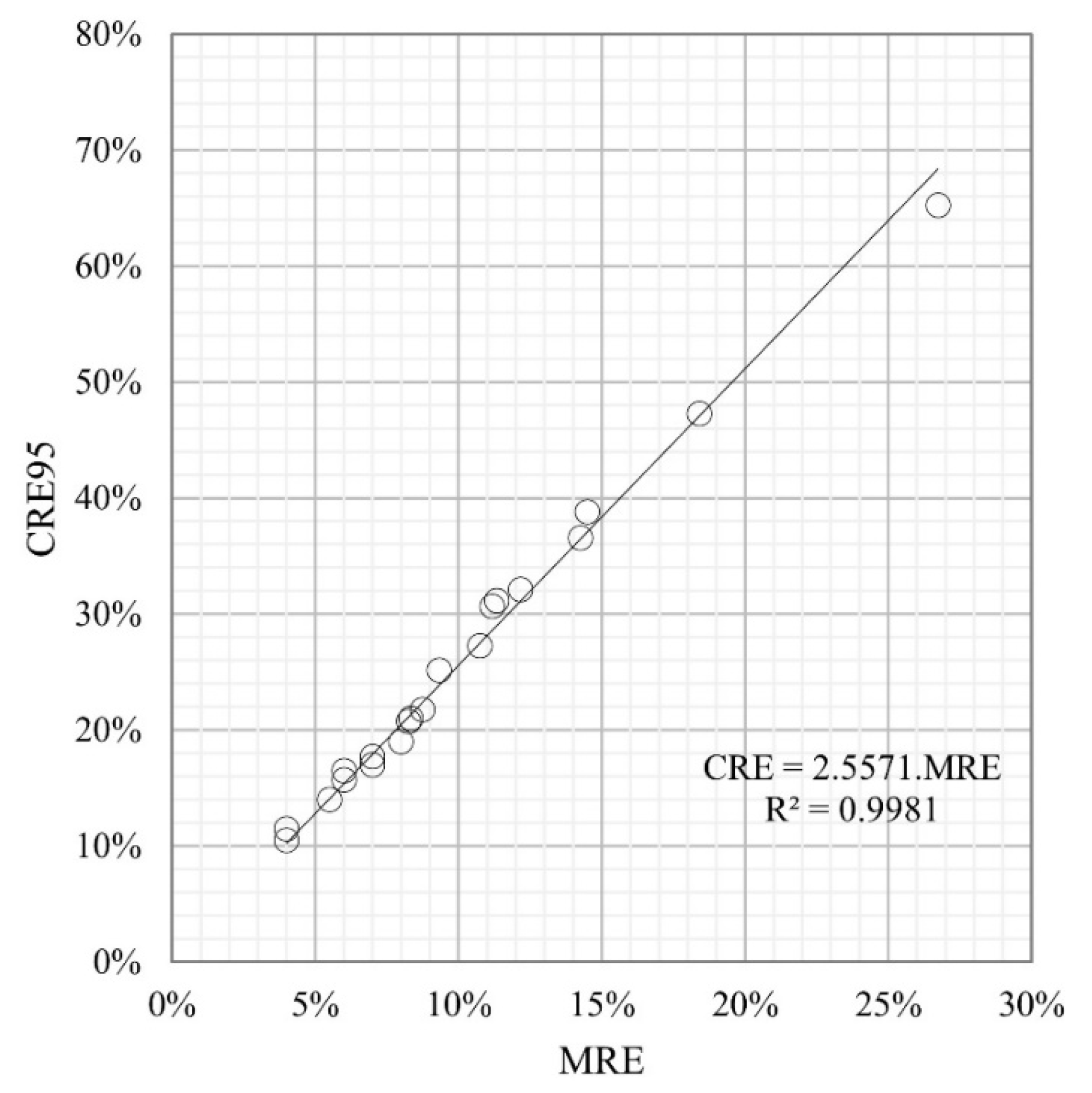
3.5. Correlation between MRE and P₉₅RE

To evaluate the error made when using this function, it can be interesting to compute the 95th percentile relative error (P₉₅RE) since for high stakes places regarding air pollution, it can be preferable to overestimate the pollution to be assured that the people in the area will not be confronted to pollution higher than what was expected. It was found that the 95th percentile relative error is linked for every relationship between monthly and annual concentration by 2.6 for PM₁₀ as well as for PM_2.5, as shown in Figure 8. For example, if there is an MRE of 10% it means that the P₉₅RE is about 26%.

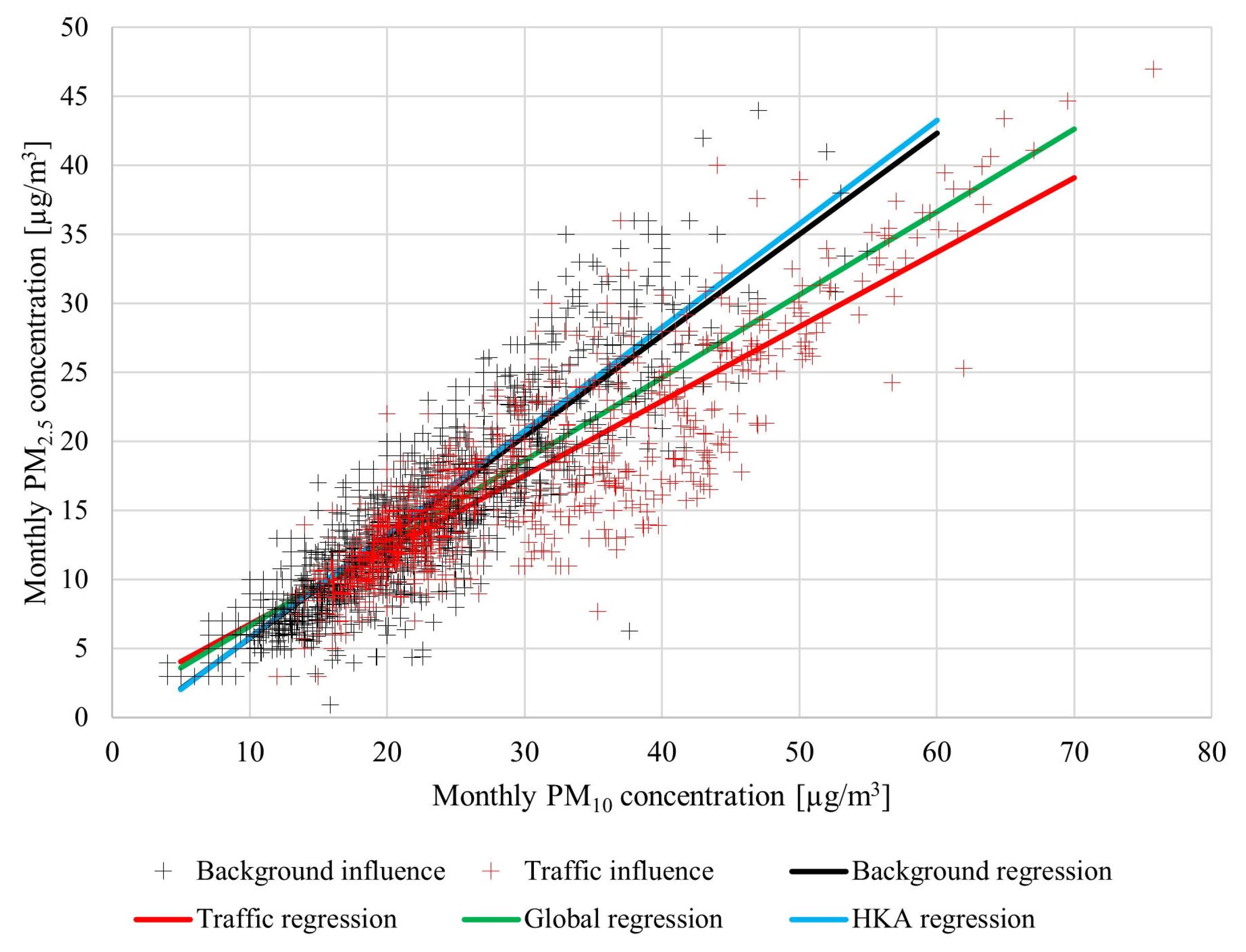
3.6. Correlation between PM₁₀ and PM_2.5 Annual Concentrations

An issue that can often happen is that a monitoring site has only data for one of the two types of particles. France is a great example of that issue as can be seen with the number of data, France is better covered for PM₁₀ than PM_2.5. So, is it possible to have an idea of the concentration of PM_2.5 from PM₁₀ and, reciprocally, PM₁₀ from PM_2.5 if the data are missing?

The data from monthly concentrations when both sensors existed were merged to be compared for a total of 2941 concentrations. The ratio between PM₁₀ and PM_2.5 vary depending on the emission sources, to evaluate this impact, the data were labeled according to their emission type (either traffic or background). The data range is from 0 to 76 µg/m³ for PM₁₀ and 0 to 47 µg/m³ for PM_2.5. However, around 90% of the background data is under 30 µg/m³ PM₁₀ and 65% for traffic data, which may influence the regression. The plot is presented in Figure 9.

The relationship obtained from the data are given in the following

Table 2. Results of the different linear regressions on the full dataset, the background and traffic influence.

Influence Type	Equation	R2	MRE	P95RE
Full dataset	PM2.5 = 0.60 × PM10 + 0.63 (5)	0.74	0.17	0.50
Background	PM2.5 = 0.73 × PM10 − 1.58 (6)	0.77	0.15	0.42
Traffic	PM2.5 = 0.54 × PM10 + 1.36 (7)	0.75	0.17	0.44

. This relationship can be used when no better data is available to evaluate the missing PM₁₀ or PM_2.5 concentrations.

The regressions obtained in this study are consistent with previous work. For instance, the report from the U.S. Environmental Protection Agency 2003 Air Quality Criteria for Particulate Matter shows a PM_2.5/PM₁₀ ratio of 0.75 for the Eastern United States, 0.52 for the Central United States, and 0.53 for the Western United States. The relationship for the background results are very close to the results obtained from the Hong Kong Environmental Protection Department [34] which they used 10 years (from 2002 to 2011), and measured five stations while excluding stations that were traffic-dominant and in which they reported the following relationship for the daily concentrations:

PM_2.5 = 0.75 × PM₁₀−1.72

(5)

Hence, it can probably be assumed that the monthly relationship found can also be used for daily concentrations.

Nevertheless, it can be noted that other works find significant differences between a winter and summer ratio [35,36]. Following our two types of months shown in Section 3.2, the regression presented in

Table 3. Results of the different linear regressions by month types.

Season type	Equation	R2	MRE	P95RE
Winter month (Jan, Feb, March)	PM2.5 = 0.61 × PM10 + 2.37 (9)	0.75	0.14	0.40
Rest of the year	PM2.5 = 0.51 × PM10 + 1.18 (10)	0.72	0.16	0.46

can be calculated.

The results can be improved by combining the two approaches. If the knowledge on both the influence type and month type is known, one can compute the two regressions and calculate the mean.

For instance, if a value of PM₁₀ is known to be from a traffic-related influence in a winter month, PM_2.5 = (0.54 × PM₁₀ + 1.36 + 0.61 × PM₁₀ + 2.37)/2 = 0.575 × PM₁₀ + 1.875.

This strategy enables the improvement of the results greatly with a R² of 0.80, a MRE of 0.12 and P₉₅RE of 0.33.

4. Discussion and Perspectives

The results presented here provide useful information on the behavior of PM₁₀ and PM_2.5 all around France and should also work for comparable countries based on the climate and lifestyle (i.e., the West European countries) since France has various types of climates (continental, oceanic, and Mediterranean). Nevertheless, the results are most likely not applicable everywhere. For instance, while Iran seems to have the same seasonal trends [37], India shows higher particulate matter concentrations during summer [38]. Thus, the results obtained in this study must be considered with geographic and lifestyle parameters. The proposed relationship most likely works in other places with four seasons, such as the rest of Europe, but it would need to be confirmed with local data from other countries. In countries with a completely different climate, the reasoning could be applied if data are available to determine the correct local regressions. The relationship described here between PM₁₀ and PM_2.5 most likely works in other parts of the world since it is in accordance with results from a previous study in China and the United States. A second limit of the results proposed here are the ranges of values. Using the regressions outside the range in extrapolation may lead to greater errors. Therefore, another perspective would be to have wider ranges of values to see if the relationship still works for higher values.

The strategy elected (number of months, each year vs. all year) to measure the annual concentration depends on two parameters: the needs and risk acceptance. Indeed, when using one month, the winter months gives the worst results. Nevertheless, it is often preferable to overestimate pollution for safety reasons for the inhabitants. Therefore, it could be a strategy to measure only in winter as it does overestimate the annual concentration generally using the raw value of measurement without applying the regression law given in the appendices. The results on using a group of months give quantitative information about it. Indeed, the MRE gives an idea of the mean error that can be made depending on the number of months elected: if the user aims to be below 10%, two months of monitoring must at least be performed. Nevertheless, it is only representative of the mean result, but for safety measures, it may be required to be sure not to underestimate the annual concentration and, thus, choosing another indicator. In such case, considering the dispersion and the chances of having an underestimation, the P₉₅RE may be used to lower the chances of underestimating the pollutant concentrations.

5. Conclusions

This work studies the assessment of annual particulate matter PM₁₀ and PM_2.5 with partial data around two aspects. First, by determining the annual concentration with monthly concentrations. Second, the relationship between PM₁₀ and PM_2.5 in France and in the world considering previous works from other authors. The main conclusions are as follows:

(a)

There is no general trend to assess particulate matter annual concentrations from any month;

(b)

Two types of behavior are highlighted regarding monthly concentrations against annual ones: winter months that overestimate annual concentrations, and the months from the rest of the year that underestimate;

(c)

Multiple months can be used to improve results, with a stronger gain in accuracy using up to 3 months than from 3 months to 6 months of monitoring;

(d)

The error of the predictions can be reduced when using two months by weighting a winter month if present by 1/4 while the other month is weighted by ¾;

(e)

The choice of strategy to assess mean annual particulate matter concentrations should be done depending on the risk acceptance and cost of campaign measurement;

(f)

If no better option is available, PM₁₀ and PM_2.5 can determine the other using a linear law depending on the influence of the station and the month.

The perspective of this work could be to compare the monthly/annual concentration results with other countries, applying the same methodology to other pollutants (except for NO₂/NO_x that were already tested in a previous work) and improving the range of concentration of particulate matter to be able to apply these solutions in more polluted areas.

References

1. WHO. Air Quality Guidelines for Particulate Matter, Ozone, Nitrogen Dioxide and Sulfur Dioxide. Global Update 2005; World Health Organization: Geneva, Switzerland, 2005. [Google Scholar]
2. He, Y.; Jiang, Y.; Wang, Y.; Yang, Y.; Xu, J.; Zhang, Y.; Wang, Q.; Shen, H.; Zhang, Y.; Yan, D.; et al. Composition of Fine Particulate Matter and Risk of Preterm Birth: A Nationwide Birth Cohort Study in 336 Chinese Cities. J. Hazard. Mater. 2021, 425, 127645. [Google Scholar] [CrossRef]
3. Lin, L.-Z.; Zhan, X.-L.; Jin, C.-Y.; Liang, J.-H.; Jing, J.; Dong, G.-H. The Epidemiological Evidence Linking Exposure to Ambient Particulate Matter with Neurodevelopmental Disorders: A Systematic Review and Meta-Analysis. Environ. Res. 2022, 209, 112876. [Google Scholar] [CrossRef] [PubMed]
4. Wang, H.; Zhang, H.; Li, J.; Liao, J.; Liu, J.; Hu, C.; Sun, X.; Zheng, T.; Xia, W.; Xu, S.; et al. Prenatal and Early Postnatal Exposure to Ambient Particulate Matter and Early Childhood Neurodevelopment: A Birth Cohort Study. Environ. Res. 2022, 210, 112946. [Google Scholar] [CrossRef] [PubMed]
5. Deary, M.E.; Griffiths, S.D. A Novel Approach to the Development of 1-hour Threshold Concentrations for Exposure to Particulate Matter during Episodic Air Pollution Events. J. Hazard. Mater. 2021, 418, 126334. [Google Scholar] [CrossRef] [PubMed]
6. Ziou, M.; Tham, R.; Wheeler, A.J.; Zosky, G.R.; Stephens, N.; Johnston, F.H. Outdoor Particulate Matter Exposure and Upper Respiratory Tract Infections in Children and Adolescents: A Systematic Review and Meta-Analysis. Environ. Res. 2022, 210, 112969. [Google Scholar] [CrossRef]
7. Anderson, J.O.; Thundiyil, J.G.; Stolbach, A. Clearing the Air: A Review of the Effects of Particulate Matter Air Pollution on Human Health. J. Med. Toxicol. 2012, 8, 166–175. [Google Scholar] [CrossRef] [PubMed] [Green Version]
8. Kim, K.-H.; Kabir, E.; Kabir, S. A Review on the Human Health Impact of Airborne Particulate Matter. Environ. Int. 2015, 74, 136–143. [Google Scholar] [CrossRef] [PubMed]
9. European Environment Agency. Air Quality in Europe: 2019 Report; European Environment Agency: Copenhagen, Denmark, 2019; ISBN 978-92-9480-088-6. [Google Scholar]
10. Karagulian, F.; Belis, C.A.; Dora, C.F.C.; Prüss-Ustün, A.M.; Bonjour, S.; Adair-Rohani, H.; Amann, M. Contributions to Cities’ Ambient Particulate Matter (PM): A Systematic Review of Local Source Contributions at Global Level. Atmos. Environ. 2015, 120, 475–483. [Google Scholar] [CrossRef]
11. Mogireddy, K.; Devabhaktuni, V.; Kumar, A.; Aggarwal, P.; Bhattacharya, P. A New Approach to Simulate Characterization of Particulate Matter Employing Support Vector Machines. J. Hazard. Mater. 2011, 186, 1254–1262. [Google Scholar] [CrossRef]
12. European Union. Directive 2008/50/EC of the European Parliament and of the Council of 21 May 2008 on Ambient Air Quality and Cleaner Air for Europe; European Union: Brussels, Belgium, 2008. [Google Scholar]
13. WHO. WHO Global Air Quality Guidelines: Particulate Matter (PM2.5 and PM10), Ozone, Nitrogen Dioxide, Sulfur Dioxide and Carbon Monoxide; World Health Organization: Geneva, Switzerland, 2021; ISBN 978-92-4-003422-8. [Google Scholar]
14. Reiminger, N.; Vazquez, J.; Blond, N.; Dufresne, M.; Wertel, J. CFD Evaluation of Mean Pollutant Concentration Variations in Step-down Street Canyons. J. Wind Eng. Ind. Aerodyn. 2020, 196, 104032. [Google Scholar] [CrossRef]
15. Rivas, E.; Santiago, J.L.; Lechón, Y.; Martín, F.; Ariño, A.; Pons, J.J.; Santamaría, J.M. CFD Modelling of Air Quality in Pamplona City (Spain): Assessment, Stations Spatial Representativeness and Health Impacts Valuation. Sci. Total Environ. 2019, 649, 1362–1380. [Google Scholar] [CrossRef] [PubMed]
16. Santiago, J.-L.; Buccolieri, R.; Rivas, E.; Sanchez, B.; Martilli, A.; Gatto, E.; Martín, F. On the Impact of Trees on Ventilation in a Real Street in Pamplona, Spain. Atmosphere 2019, 10, 697. [Google Scholar] [CrossRef] [Green Version]
17. Fiates, J.; Vianna, S.S.V. Numerical Modelling of Gas Dispersion Using OpenFOAM. Process Saf. Environ. Prot. 2016, 104, 277–293. [Google Scholar] [CrossRef]
18. Vranckx, S.; Vos, P.; Maiheu, B.; Janssen, S. Impact of Trees on Pollutant Dispersion in Street Canyons: A Numerical Study of the Annual Average Effects in Antwerp, Belgium. Sci. Total Environ. 2015, 532, 474–483. [Google Scholar] [CrossRef]
19. Hagler, G.S.W.; Lin, M.-Y.; Khlystov, A.; Baldauf, R.W.; Isakov, V.; Faircloth, J.; Jackson, L.E. Field Investigation of Roadside Vegetative and Structural Barrier Impact on Near-Road Ultrafine Particle Concentrations under a Variety of Wind Conditions. Sci. Total Environ. 2012, 419, 7–15. [Google Scholar] [CrossRef] [PubMed]
20. Lee, E.S.; Ranasinghe, D.R.; Ahangar, F.E.; Amini, S.; Mara, S.; Choi, W.; Paulson, S.; Zhu, Y. Field Evaluation of Vegetation and Noise Barriers for Mitigation of Near-Freeway Air Pollution under Variable Wind Conditions. Atmos. Environ. 2018, 175, 92–99. [Google Scholar] [CrossRef]
21. Reiminger, N.; Jurado, X.; Vazquez, J.; Wemmert, C.; Blond, N.; Dufresne, M.; Wertel, J. Effects of Wind Speed and Atmospheric Stability on the Air Pollution Reduction Rate Induced by Noise Barriers. J. Wind Eng. Ind. Aerodyn. 2020, 200, 104160. [Google Scholar] [CrossRef]
22. Tong, Z.; Baldauf, R.W.; Isakov, V.; Deshmukh, P.; Max Zhang, K. Roadside Vegetation Barrier Designs to Mitigate Near-Road Air Pollution Impacts. Sci. Total Environ. 2016, 541, 920–927. [Google Scholar] [CrossRef]
23. Wang, S.; Wang, X. Modeling and Analysis of the Effects of Noise Barrier Shape and Inflow Conditions on Highway Automobiles Emission Dispersion. Fluids 2019, 4, 151. [Google Scholar] [CrossRef] [Green Version]
24. Yu, Y.; Kwok, K.C.S.; Liu, X.P.; Zhang, Y. Air Pollutant Dispersion around High-Rise Buildings under Different Angles of Wind Incidence. J. Wind Eng. Ind. Aerodyn. 2017, 167, 51–61. [Google Scholar] [CrossRef]
25. Aristodemou, E.; Boganegra, L.M.; Mottet, L.; Pavlidis, D.; Constantinou, A.; Pain, C.; Robins, A.; ApSimon, H. How Tall Buildings Affect Turbulent Air Flows and Dispersion of Pollution within a Neighbourhood. Environ. Pollut. 2018, 233, 782–796. [Google Scholar] [CrossRef] [PubMed]
26. Calzolari, G.; Liu, W. Deep Learning to Replace, Improve, or Aid CFD Analysis in Built Environment Applications: A Review. Build. Environ. 2021, 206, 108315. [Google Scholar] [CrossRef]
27. Jurado, X.; Reiminger, N.; Benmoussa, M.; Vazquez, J.; Wemmert, C. Deep Learning Methods Evaluation to Predict Air Quality Based on Computational Fluid Dynamics. Expert Syst. Appl. 2022, 203, 117294. [Google Scholar] [CrossRef]
28. Jurado, X.; Reiminger, N.; Vazquez, J.; Wemmert, C. On the Minimal Wind Directions Required to Assess Mean Annual Air Pollution Concentration Based on CFD Results. Sustain. Cities Soc. 2021, 71, 102920. [Google Scholar] [CrossRef]
29. Reiminger, N.; Jurado, X.; Vazquez, J.; Wemmert, C.; Dufresne, M.; Blond, N.; Wertel, J. Methodologies to Assess Mean Annual Air Pollution Concentration Combining Numerical Results and Wind Roses. Sustain. Cities Soc. 2020, 59, 102221. [Google Scholar] [CrossRef]
30. Jurado, X.; Reiminger, N.; Vazquez, J.; Wemmert, C.; Dufresne, M.; Blond, N.; Wertel, J. Assessment of Mean Annual NO2 Concentration Based on a Partial Dataset. Atmos. Environ. 2020, 221, 117087. [Google Scholar] [CrossRef]
31. Li, C.; Liu, M.; Hu, Y.; Zhou, R.; Huang, N.; Wu, W.; Liu, C. Spatial Distribution Characteristics of Gaseous Pollutants and Particulate Matter inside a City in the Heating Season of Northeast China. Sustain. Cities Soc. 2020, 61, 102302. [Google Scholar] [CrossRef]
32. Miao, C.; Yu, S.; Hu, Y.; Liu, M.; Yao, J.; Zhang, Y.; He, X.; Chen, W. Seasonal Effects of Street Trees on Particulate Matter Concentration in an Urban Street Canyon. Sustain. Cities Soc. 2021, 73, 103095. [Google Scholar] [CrossRef]
33. Anjum, M.S.; Ali, S.M.; Imad-ud-din, M.; Subhani, M.A.; Anwar, M.N.; Nizami, A.-S.; Ashraf, U.; Khokhar, M.F. An Emerged Challenge of Air Pollution and Ever-Increasing Particulate Matter in Pakistan; A Critical Review. J. Hazard. Mater. 2021, 402, 123943. [Google Scholar] [CrossRef]
34. Environmental Protection Department. Guidelines on the Estimation of PM2.5 for Air Quality Assessment in Hong Kong; Environmental Protection Department: Hong Kong, China, 2012. [Google Scholar]
35. Harrison, R.M.; Deacont, A.R.; Jones, M.R. Sources and Processes Affecting Concentrations of Pmlo and Pm2.5 Particulate Matter in Birmingham (U.K.). Atmos. Environ. 1997, 31, 4103–4117. [Google Scholar] [CrossRef]
36. Romieu, I.; Borja-Aburto, V.H. Particulate Air Pollution and Daily Mortality: Can Results Be Generalized to Latin American Countries? Salud. Pública Méx. 1997, 39, 403–411. [Google Scholar] [CrossRef] [PubMed]
37. Jafari, A.J.; Delikhoon, M.; Rastani, M.J.; Baghani, A.N.; Sorooshian, A.; Rohani-Rasaf, M.; Kermani, M.; Kalantary, R.R.; Golbaz, S.; Golkhorshidi, F. Characteristics of Gaseous and Particulate Air Pollutants at Four Different Urban Hotspots in Tehran, Iran. Sustain. Cities Soc. 2021, 70, 102907. [Google Scholar] [CrossRef]
38. Ganguly, R.; Sharma, D.; Kumar, P. Trend Analysis of Observational PM10 Concentrations in Shimla City, India. Sustain. Cities Soc. 2019, 51, 101719. [Google Scholar] [CrossRef]
Figure 1. Location of the regions where data were used.
Atmosphere 14 00385 g001
Figure 2. PM10 and PM2.5 general evolution (A) as a function of the years (with mean annual concentrations following the red line) and detail of the influence for PM10 (B) and PM2.5 (C).
Atmosphere 14 00385 g002
Figure 3. Evolution of the PM10 annual concentration as a function of the monthly concentration considering (A) the whole dataset and (B) only the year 2019, and their corresponding linear regressions.
Atmosphere 14 00385 g003
Figure 4. Months clustering according to the comparison of annual and monthly concentrations: (A) clustering results of PM10, (B) PM2.5, and (C) R2 from linear regression depending on the months for PM2.5 (light gray) and PM10 (dark gray).
Atmosphere 14 00385 g004
Figure 5. Comparison of the MRE when considering for each month, all the years at once, or one year at a time independently (average result) for PM10 (left) and PM2.5 (right).
Atmosphere 14 00385 g005
Figure 6. Evolution of the mean relative error (A) depending on the number of months for PM10 (left) and PM2.5 (right) when using the linear regression and directly averaging.
Atmosphere 14 00385 g006
Figure 7. Improvement of the mean absolute error when weighting by ¼ the winter month and rest of the year by ¾ for PM10 (left) and PM2.5 (right).
Atmosphere 14 00385 g007
Figure 8. Relationship between mean error and 95th percentile error.
Atmosphere 14 00385 g008
Figure 9. Monthly concentration of PM2.5 against monthly concentration of PM10.
Atmosphere 14 00385 g009