Abstract
Field calibration of low-cost air quality (AQ) monitoring sensors is essential for their successful operation. Low-cost sensors often exhibit non-linear responses to air pollutants and their signals may be affected by the presence of multiple compounds making their calibration challenging. We investigate different approaches for the field calibration of an AQ monitoring device named ENSENSIA, developed in the Institute of Chemical Engineering Sciences in Greece. The present study focuses on the measurements of two of the most important pollutants measured by ENSENSIA: NO2 and O3. The measurement site is located in the center of Patras, the third biggest city in Greece. Reference instrumentation used for regulatory purposes by the Region of Western Greece was used as the evaluation standard. The sensors were installed for two years at the same locations. Measurements from the first year (2021) from seven ENSENSIA sensors (NO2, NO, O3, CO, PM2.5, temperature and relative humidity) were used to train several Machine Learning (ML) and Deep Learning (DL) algorithms. The resulting calibration algorithms were assessed using data from the second year (2022). The Random Forest algorithm exhibited the best performance in correcting O3 and NO2. For NO2 the mean error was reduced from 9.4 ppb to 3 ppb, whilst R2 improved from 0.22 to 0.86. Similar results were obtained for O3, wherein the mean error was reduced from 13 to 4.3 ppb and R2 increased from 0.52 to 0.69. The Long-Short Term Memory Network (LSTM) also showed good performance in correcting the measurements of the two pollutants.
1. Introduction
Monitoring outdoor and indoor air quality (AQ) is an urgent need in the developed and developing world [1]. Real-time monitoring can provide many societal benefits and help improve human health. Knowledge of the prevailing AQ conditions can reduce respiratory, cardiovascular and other problems [2,3], especially for sensitive groups.
Two major gaseous pollutants affecting human health are ozone (O3) and nitrogen dioxide (NO2). Ozone has been found to trigger various health problems, such as chest pain, coughing, throat irritation, and congestion. Bronchitis, asthma, and emphysema can worsen due to exposure to high ozone levels. Long-time repeated exposure to ozone may permanently scar the lung tissues [4]. Nitrogen dioxide also has a range of harmful effects on our lungs, including (i) increased inflammation of the airways; (ii) cough and wheezing; (iii) reduced lung function; (iv) increased asthma attacks, and (v) greater likelihood of emergency department and hospital admissions [5]. Asthmatics, children, and older adults are especially sensitive to these air pollutants.
Monitoring gaseous pollutant concentrations across wide areas is costly and requires sensitive instruments and the corresponding infrastructure for the monitoring stations. Deploying several monitoring stations becomes prohibitively expensive for large urban and industrial areas [6]. In addition, precision instruments can cost tens of thousands of euros [1].
Several low-cost sensors have recently been developed to record and monitor gaseous pollutants and aerosols. These sensors are characterized as low-cost, and their name suggests their main benefit. Low-cost sensors have attracted the interest of the research community, regulatory bodies, and companies [7,8,9]. Despite their disadvantages, such as low accuracy, frequent errors, and periods of instability [10], these sensors are certainly a major step in the effort to monitor AQ with high spatial resolution in large urban areas, but also to start air pollutant measurements in some parts of the developing world.
Data analytics and low-cost sensor reading corrections are topics of current research. Popular low-cost sensors such as the Alphasense NO2-B43F and OX-B431, which measure NO2 and O3, respectively, occasionally exhibit a non-linear relationship with the reference measurements. Our hypothesis in this work is that the raw measurements of low-cost sensors can be corrected with the aid of Machine Learning (ML) and Deep Learning (DL) algorithms to attain an acceptable agreement with the ground truth.
Several recent studies have assessed the performance of NO2-B43F and OX-B431 sensors. Zimmerman et al. [11] trained and tested Random Forest (RF) and Multiple Linear Regression (MLR) models for a six-month period in Pittsburgh. They reported that the RF algorithm was suitable for calibrating the two sensor types by integrating the raw sensor responses of all the deployed sensor types (CO-B4, COZIR-2000 CO2, NO2-B43F, and OX-B431), as well as the ambient temperature and relative humidity. The RF-calibrated NO2 and O3 concentrations exhibited an R2 of 0.62 and 0.86, respectively.
Ratingen et al. [12] employed MLR to calibrate the NO2-B43F sensor using the raw NO2-B43F, OX-B431 measurements, and ambient temperature as inputs in the Netherlands. The calibration methodology was evaluated based on a ten-fold cross-validation procedure. MLR improved the R2 of hourly measurements from 0.54 to 0.69–0.84. Han et al. [13] collocated Alphasense B4 sensors for CO, NO2, O3, and SO2 in Beijing. They used the working and auxiliary electrode signals in conjunction with the temperature and relative humidity to evaluate MLR, RF, and Long-Short Term Memory (LSTM) algorithms. RF and LSTM increased the R2 from 0.3–0.5 to 0.7 for both O3 and NO2.
Christakis et al. [14] used linear corrections for an NO2 (NO2-B43F) and an O3 (OX-B431) sensor in Athens. The linear calibration for each sensor integrated the sensor’s working and auxiliary electrode signals, along with a temperature-compensation factor. R2 increased from 0.45 to 0.84 for the NO2 sensor and from 0.61 to 0.87 for the O3 sensor. Margaritis et al. [15] reported that the RF algorithm had better performance than other algorithms tested in Thessaloniki, Greece improving R2 for both sensors (NO2-B43F, OX-B431) to 0.92 and 0.96, respectively.
The Institute of Chemical Engineering Sciences (ICE-HT) has developed a low-cost AQ monitoring device, ENSENSIA, equipped with low-cost sensors for several air pollutants including NO2 and O3. The device is analytically described in [16]. In our previous work, the proposed device completed the preliminary tests, which included stability and continuous operation experiments, and reading agreement with equivalent low-cost commercially available devices. In this work, we present the results of the field calibration of ENSENSIA for NO2 and O3. The device was co-located with reference instrumentation provided by the Region of Western Greece at the center of Patras, Greece. The period of the measurements (1/1/2021 to 30/10/2022) covers all seasons and meteorological conditions for a typical city in southeastern Europe.
We present and discuss the operation, the advantages, and the limitations of several ML and DL algorithms that were used to correct the readings of our device. The conducted tests reveal that the low-cost sensor readings can indeed be improved with the use of such algorithms, especially with the development of ensemble methodologies.
2. Materials and Methods
2.1. Environment Sensing Appliance (ENSENSIA)
The low-cost sensor device of the current study entitled “ENSENSIA” has been developed by FORTH/ICE-HT and is analytically described in [16]. ENSENSIA includes aerosol, gas and meteorological sensors to measure fine particulate matter (PM2.5, mass of particle with diameter smaller than 2.5 μm), ozone, nitrogen oxide and dioxide, and carbon monoxide. Table 1 summarises the types of ENSENSIA sensors.

Table 1.
Description of the low-cost sensors installed in ENSENSIA in this study.
It is a Raspberry PI-based device that offers several edge-computing opportunities, stability of use, and remote control.
2.2. Measurement Site
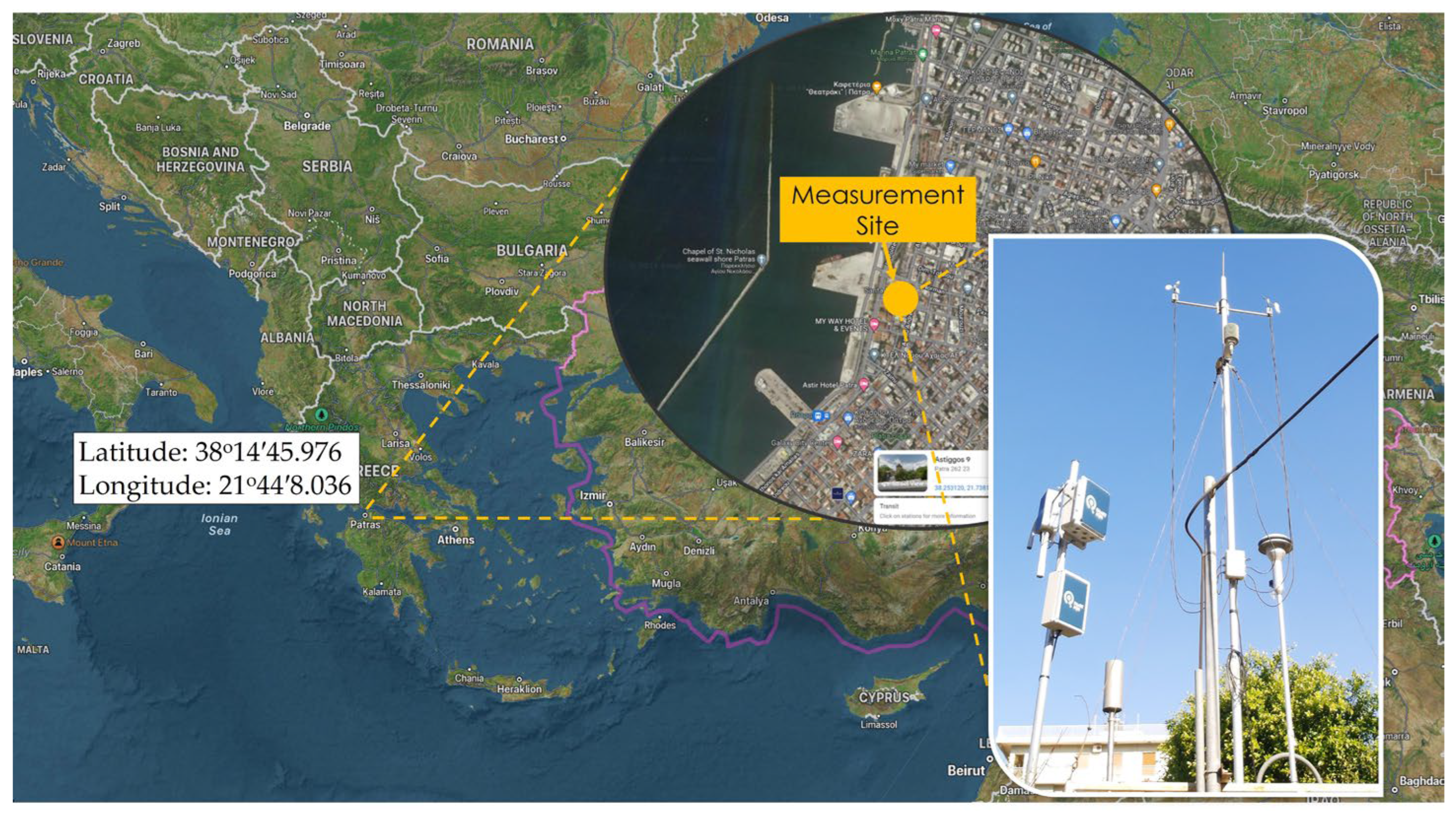
The urban background measurement site is located in the center of Patras, Greece, at latitude 38°14′45.976″ and longitude 21°44′8.036″ (Figure 1). ENSENSIA was placed on the roof of a small structure used as a regulatory AQ monitoring station by the Region of Western Greece. The device was placed approximately 6 m above ground and next to the inlets of the reference monitors. The reference monitor is the model HORIBA 360, which measures CO, SO2, NOx, and O3.

Figure 1.
Map and photos of the measurement site in Patras, Greece.
Measurements by ENSENSIA and the regulatory monitors over a 22-month period starting on 1 January 2021 to 30 October 2022 are analyzed in the present work.
2.3. Data Preprocessing
The device’s sensors measure every 10 s and report their average measurements every 2 min. ENSENSIA is configured to provide a collection of the sensors’ readings every two minutes, and its operation is continuous. For the data analysis of the present study, the hourly averages of ENSENSIA readings are used. All gas-phase concentrations are reported as molecular mixing ratios in parts per billion (ppb) units.
All sensor readings and the corresponding reference concentrations were stored in a MySQL database after processing the output files of the reference monitors. ENSENSIA reported its readings directly to the database.
During the analysis, outlier values of both the regulatory instrumentation and ENSENSIA have been removed. Negative and missing values were excluded from the analysis.
The resulting data completeness over the 22-month period, was 91.8% for the ENSENSIA device and 91.2% for the reference instrumentation. The aggregation yielded a completeness of 88.5%.
We considered all available sensor readings for applying ML and DL algorithms when correcting either NO2 or O3. Subsequently, the input data of the algorithms include all the NO2, O3, NO, CO, PM2.5, T, and RH values, as reported by ENSENSIA. The measurements reported by the regulatory instrumentation are considered as the ground truth.
2.4. Machine Learning and Deep Learning
The present study evaluates several ML and DL methods to correct the measured gas concentrations based on their reference counterparts. Conventional methods and ML and DL methods are employed to correct the readings of the low-cost device. In the following paragraphs, brief descriptions of these methods are provided.
2.4.1. Linear Correction
A linear relation between the reference concentration and the multiple low-cost sensor readings was assumed in this approach:
where “raw” denotes the uncorrected low-cost sensor readings.
2.4.2. K-Nearest Neighbors
The k-nearest neighbors (KNN) algorithm is one of the most naïve ML algorithms. KNN uses feature similarity to estimate the value of the new data points based on how closely they resemble the points in the training set [17]. KNN computes the distance between the new points and the training data points to achieve this. Several methods calculate the distance between data points, including Euclidean, Manhattan, and Hamming distances. The hyperparameter k, which is included in the name of the method, refers to the number of neighbors used to estimate any new point’s value. The corrected concentration value of NO2 is expected to fall near the closest neighbor, i.e., the set of NO2, NO, CO, O3, T, RH, PM2.5 which is most similar to the set under investigation. The Euclidean distance was used for the analysis.
One of the main setbacks of KNN is that it is sensitive to outliers as it chooses the neighbors based on distance criteria. Table 2 presents the KNN parameters tuned for this study.
Table 2.
Parameters and hyper-parameters of the ML and DL models.
2.4.3. Random Forest
Random Forest is an ensemble learning method for classification and regression [18]. It constructs several decision trees (estimators) that process the input data and provide their predictions independently. Each decision tree aims to reveal rules that match the observed concentrations (x) to the expected concentrations (y). For example, a tree may declare that when x is below a specific threshold (e.g., 5 ppb), it will be treated differently from the rest of the input data. This is called a split. The decision tree may perform many similar splits. In problems involving many attributes, the decision tree may perform such splits using those attributes. The algorithm receives a set of inputs to correct the O3 readings. In our case, those inputs include all the ENSENSIA readings (CO, NO, NO2, O3, T, RH, PM2.5). RF constructs several trees (estimators) and trains them to estimate the “correct” ozone concentration. The latter is an ensemble of decision trees, which constitute the “forest”. Usually, those trees are trained with the bagging method [19]. RF introduces randomness to its operation. Each estimator is trained on subsets of the initial data (bootstrap method) and becomes a specialized, but weak, learner. The general idea of the bagging method is that a combination of learning models improves the overall result. RF aggregates the predicted concentrations provided by the decision trees. The final prediction can be decided by several methods, such as majority voting or mean [20]. RF is expected to perform the necessary splits to predict the reference concentration, but also to determine the importance of each feature to the algorithm’s decision. In its current implementation, RF consists of 1000 estimators, which are selected by performing extensive tests using the grid-search algorithm. The importance of each feature is reported and used to verify the cross-sensitivity among the electrochemical sensors.
2.4.4. Artificial Neural Network
NN or Artificial NN (ANN) is a network of neurons. Its architecture is inspired by the biological functions of the human brain. Each node or artificial neuron connects to another and has an associated weight and threshold [17]. If the output of any individual node is above a specified threshold value, that node is activated, sending its output to the next layer of the network. Once an input layer is determined, weights are assigned. Several hidden layers of neurons can process the input data. Neural Networks learn from the input data in batches, adjusting the neuron weights to minimize a specific error function. For air pollutant time-series, error functions usually are based on the mean absolute or the mean squared error of the predicted concentrations compared to the more accurate measurements. The proposed NN consists of an input layer of 7 nodes connected to the input variables (CO, NO, NO2, O3, T, RH, PM2.5). Two hidden layers of 24 and 48 nodes follow, in which the input variables are combined to discover inner relations among them. The output layer is a single node representing the predicted concentration. The prediction is compared to the accurate concentration (the reference) and an error is computed. This error is back-propagated to the nodes of the network, forcing the weight values to be updated in a way that the network improves its performance. Since this is performed for several data points, the algorithm needs to converge to a solution. This is achieved by the use of optimization methods that update the learning parameters. The selection of a suitable optimizer is essential to efficiently train a NN. The current NN implementation used the Stochastic Gradient Descent optimizer. Our choice was made after testing several alternative optimizers, such as Adam, RMSprop, and Adagrad for the corresponding problem.
NNs require large-scale datasets to learn effectively. The desired data size increases non-linearly with the depth of the network and the trainable parameters. Small datasets often cause the model to underfit, i.e., fail to learn, mandating the selection of a shallower network, or performing data augmentation.
Limitations of the NNs include their black-box nature, their frequent failure to generalize and predict unseen data derived from external validation tests, and their time-consuming training.
2.4.5. Long-Short Term Memory Network
LSTM is a Recurrent Neural Network [21,22] used in several DL tasks. LSTM involves feedback connections among the units, allowing the processing of entire sequences of data, rather than single data points.
The basis of a conventional LSTM cell includes four main gates: input gate, input modulation gate, forget gate and output gate. The input gate is responsible for processing incoming data points. The memory cell input gate receives the output of the LSTM cell during the last iterations. The Forget gate decides when to forget the output results and thus selects the optimal time lag for the input sequence. The output gate receives all the results from the previously mentioned gates and returns the output. LSTM operates similarly to a NN. The strongest feature of LSTM is its inherent ability to discover time-related connections between data points, which is desirable when dealing with time-series regression problems. LSTM is implemented using two units that process batches of 24 data points. To this end, after the training is complete, the prediction of the current NO2 or O3 concentration requires the current raw ENSENSIA measurement of NO2, O3, NO, CO, PM2.5, T, and RH as well as the latest 23 raw ENSENSIA measurements of NO2, O3, NO, CO, PM2.5, T, and RH. The model uses two hidden layers of 60 and 120 nodes. The error function uses the mean absolute concentration error units to update the weights. The Adam optimization algorithm was selected after tests with the Stochastic Gradient Descent, and RMSprop. The parameters of the LSTM model are presented in Table 2.
A potential weakness of this model is related to data completeness. The latest 23 ENSENSIA measurements may not correspond to uniform time intervals. As a result, unexpected data representations may appear in the trained model reducing its performance. In addition, LSTM shares the limitations of neural networks.
2.4.6. Convolutional Neural Network
CNN [23] is a well-known deep learning architecture inspired by living creatures’ natural visual perception mechanism [24]. It is a special NN type named after the linear mathematical operation between matrices called convolution. Components of CNNs include several layers, such as the convolution layer, their cornerstone, pooling and activation layers, and densely connected layers. The convolution layer is built by several convolution kernels used to compute feature maps. Specifically, each neuron of a feature map is connected to a region of neighboring neurons in the previous layer. The feature map is generated by first convolving the input with a learned kernel and then applying an element-wise non-linear activation function on the convolved results. Modern CNNs consist of convolution layers that process the input data hierarchically and learn high-level features that map those data with the desired outputs. The proposed CNN makes use of 2D convolutions to process a sequence of measurements (24), similar to the LSTM model. As a result, the input data representation is similar to an image array. The input data is progressively filtered using 24, 48, and 120 filters with a 3 × 3 kernel. The resulting one-dimensional vector is used for the regression. The mean squared error function is utilized for the weights which are updated using the Adam optimization algorithm.
CNN learning is similar to NN and shares the NN’s limitations. Table 2 presents the parameters and hyper-parameters of the implemented CNN.
2.5. Experiment Setup and Performance Metrics
Each ML and DL model is defined by several hyper-parameters, which describe its functionality and affect the performance given a specific regression task. We have performed offline parameter tuning to define the optimal values for the model’s parameters. Those are summarized Table 2.
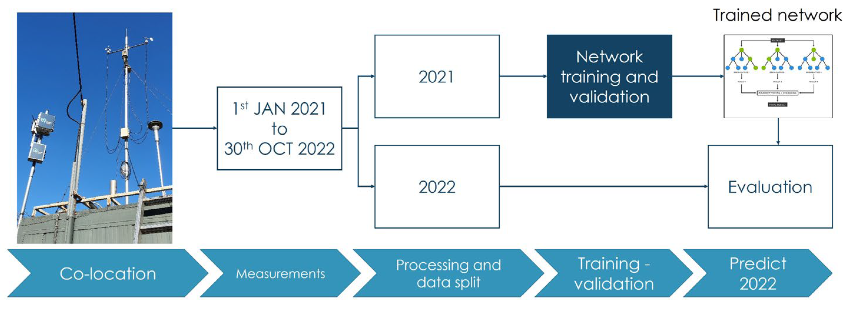
We divide the measurement period into two campaigns. The first campaign refers to 2021 and is used to train and evaluate the algorithms. The second campaign (2022) is utilized for the test set. Training and validation on the 2021 campaign are performed under a five-fold cross-validation train-test scheme, as suggested in [10]. An overview of the experiment is illustrated in Figure 2.
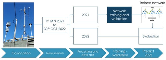
Figure 2.
Training and evaluation/validation overview.
A series of evaluation metrics are used in our analysis. The Mean Error (ME) and Root Mean Squared Error (RMSE) are accuracy metrics that give the average errors concerning the reference measurements. R (correlation coefficient) and R2 (coefficient of determination) are correlation parameters that describe the strength of the relationship between the sensor readings and the reference measurements. The normalized ME (nME) is a relative error metric that also provides useful information about the performance of our sensors and correction algorithms. Finally, mean bias (MB) quantifies the bias of the sensor. Studies suggest that at least ME, RMSE, R, R2, and nME should be reported [10].
The above metrics are calculated using the following equations:
where the n measurements of the reference instruments (observed values) are denoted by Oi and the corrected sensor values (expected values) by Ei).
3. Results
3.1. Nitrogen Dioxide
During the 2021 campaign, the observed (reference) mean and standard deviation of NO2 concentration was 12.5 ± 8.4 ppb. The minimum and maximum observed values were 1 and 44 ppb, respectively. The ML algorithms were trained under a 5-fold cross-validation procedure in the 2021 campaign.
The trained models were evaluated on the unseen data of the 2022 campaign. During this period, the observed mean and standard deviation of NO2 concentration was 12.8 ± 8.5 ppb. The minimum and maximum observed values were 0.5 and 45 ppb, respectively.
3.1.1. Evaluation of Uncorrected Sensor Readings
Considering the uncorrected measurements of ENSENSIA, the ME of the two periods were 8.6 and 9.4 ppb, respectively. Table 3 summarizes the results.
Table 3.
Evaluation metrics for the uncorrected ENSENSIA measurements of ozone against the reference. The metrics were calculated based on hourly-averaged values.
3.1.2. Evaluation of Machine Learning Algorithms
The ML algorithms were trained and validated on the 2021 Campaign under a 5-fold cross-validation procedure. The 2022 Campaign was used to assess the algorithms’ efficiency in predicting unseen data. The results are presented in Table 4.
Table 4.
Agreement metrics between the reference NO2 concentrations and the corrected ENSENSIA readings.
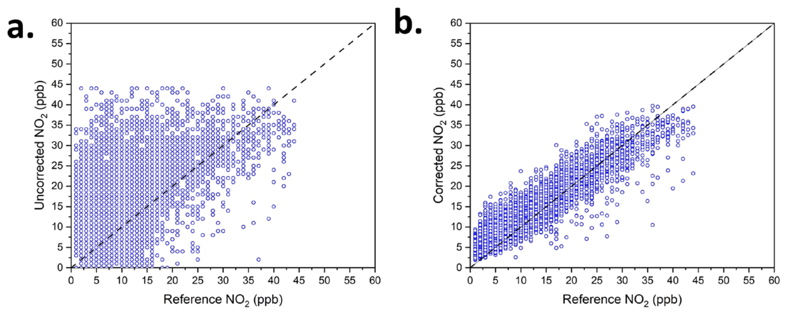
Figure 3 displays the uncorrected NO2 sensor readings versus the observed reference NO2 concentration and the RF-corrected NO2 sensor readings versus the observed reference NO2 concentration.
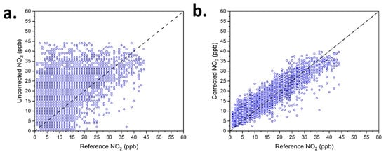
Figure 3.
(a) Uncorrected hourly NO2 sensor readings versus the observed reference NO2 concentration, (b) RF-corrected NO2 sensor readings versus the observed reference NO2 concentration. Both diagrams refer to the test set (2022).
The RF algorithm demonstrated very good performance. The uncorrected NO2 sensor reading for the test period showed a ME, R2, and nME of 9.4 ppb, 0.22, and 0.67, respectively (Table 3). After the correction with the RF algorithm, the ME, R2, and nME were 3 ppb, 0.86, and 0.3, respectively (Table 4). The LSTM algorithm also had good performance in correcting the NO2 concentrations of the test set. After the correction with the LSTM algorithm, the ME was 3 ppb, the R2 was 0.82 and nME was 0.31.
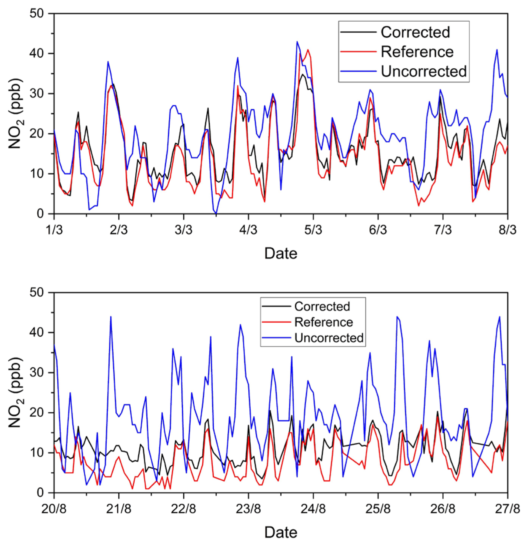
Figure 4 shows the time series of NO2 concentrations for two characteristic 7-day periods.

Figure 4.
Time series of NO2 concentrations for two 7-day periods of the test set (2022). Uncorrected NO2 low-cost sensor reading is displayed with blue lines, RF-corrected NO2 values are displayed with black lines, and reference NO2 concentrations are displayed with red lines.
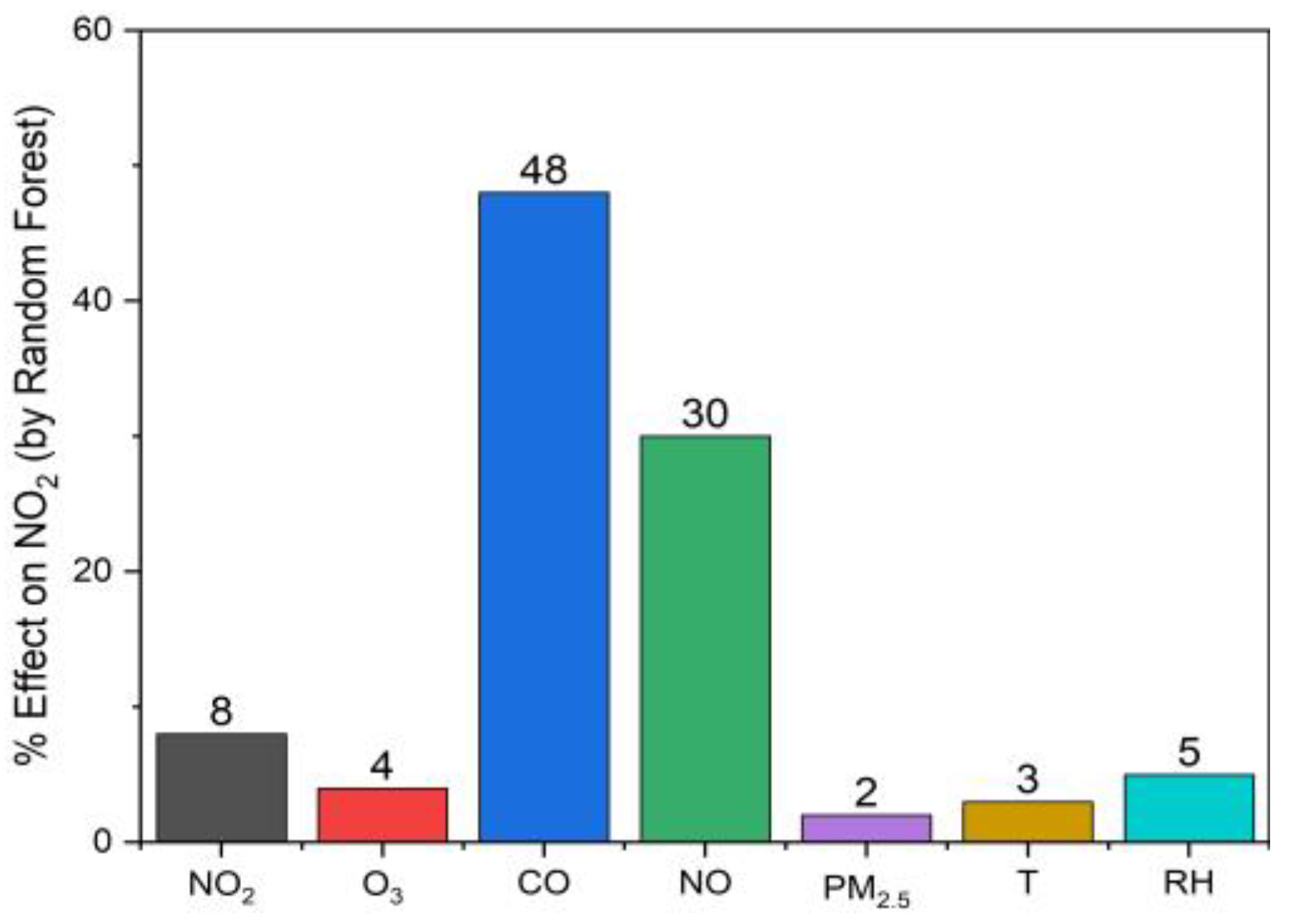
The RF algorithm also calculates the importance of each input attribute to its prediction. RF selects the raw reading of CO as its most important measurement (48% importance). The NO measurement is rated at 30%, whilst the raw NO2 reading’s importance is valued at 8%. These relations are summarized in Figure 5.

Figure 5.
The importance of the ENSENSIA readings for correcting NO2 using the RF algorithm. The importance is suggested by RF based on the training set (2021).
From this observation, we conclude that the sensors complement each other. For this reason, the correction of their measurements can be more accurate when the measurements from the desired gas and the measurements of the other sensors are taken into account.
3.2. Ozone
During the 2021 campaign, the observed mean and standard deviation of O3 concentration was 34 ± 11.8 ppb. The minimum and maximum observed values were 1 and 97 ppb, respectively. The ML algorithms were trained under a 5-fold cross-validation procedure in the 2021 campaign.
The trained models were evaluated on the unseen data of the 2022 campaign. During this period, the observed mean and standard deviation of O3 concentration was 31 ± 9.6 ppb. The minimum and maximum observed values were 1 and 96 ppb, respectively.
3.2.1. Evaluation of Uncorrected Sensor Readings
Considering the uncorrected measurements of ENSENSIA, the ME for the two periods were 13.9 and 13 ppb, respectively. Table 5 summarizes the results.
Table 5.
Evaluation metrics for the uncorrected ENSENSIA measurements of ozone against the reference. The metrics were calculated based on hourly-averaged values.
3.2.2. Evaluation of Machine Learning Algorithms
The ML algorithms were trained and validated on the 2021 Campaign under a 5-fold cross-validation procedure. The 2022 campaign was used to assess the algorithms’ efficiency in predicting unseen data.
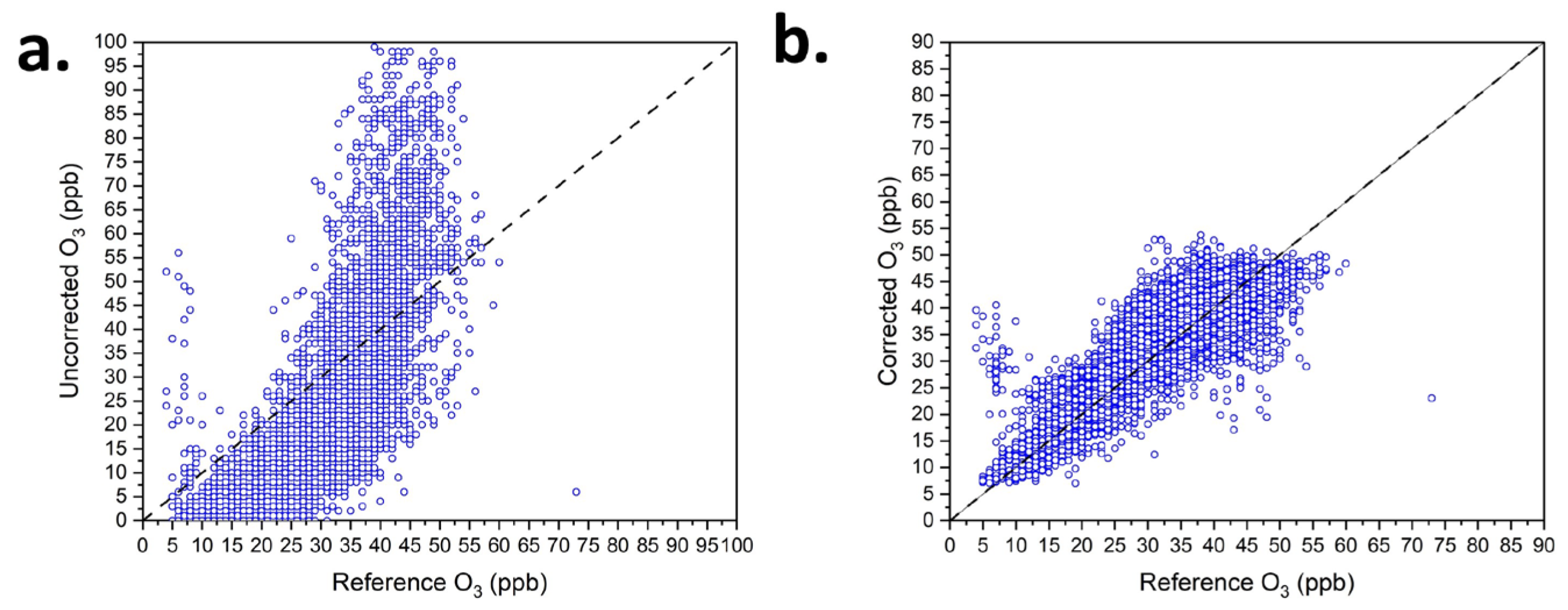
Figure 6 shows the uncorrected O3 and the RF-corrected O3 sensor readings versus the measured reference O3 concentration. Figure 7 presents time series of O3 concentrations for two 7-day periods.
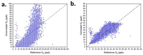
Figure 6.
(a) Uncorrected O3 sensor readings versus the observed reference NO2 concentration, (b) RF-corrected O3 sensor readings versus the observed reference O3 concentration. Both diagrams refer to the test year (2022).
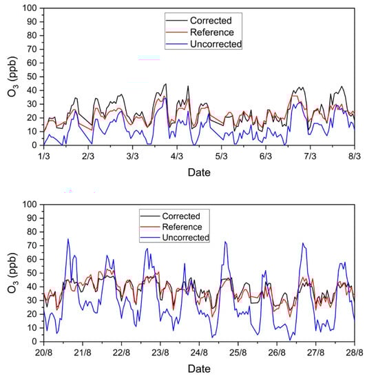
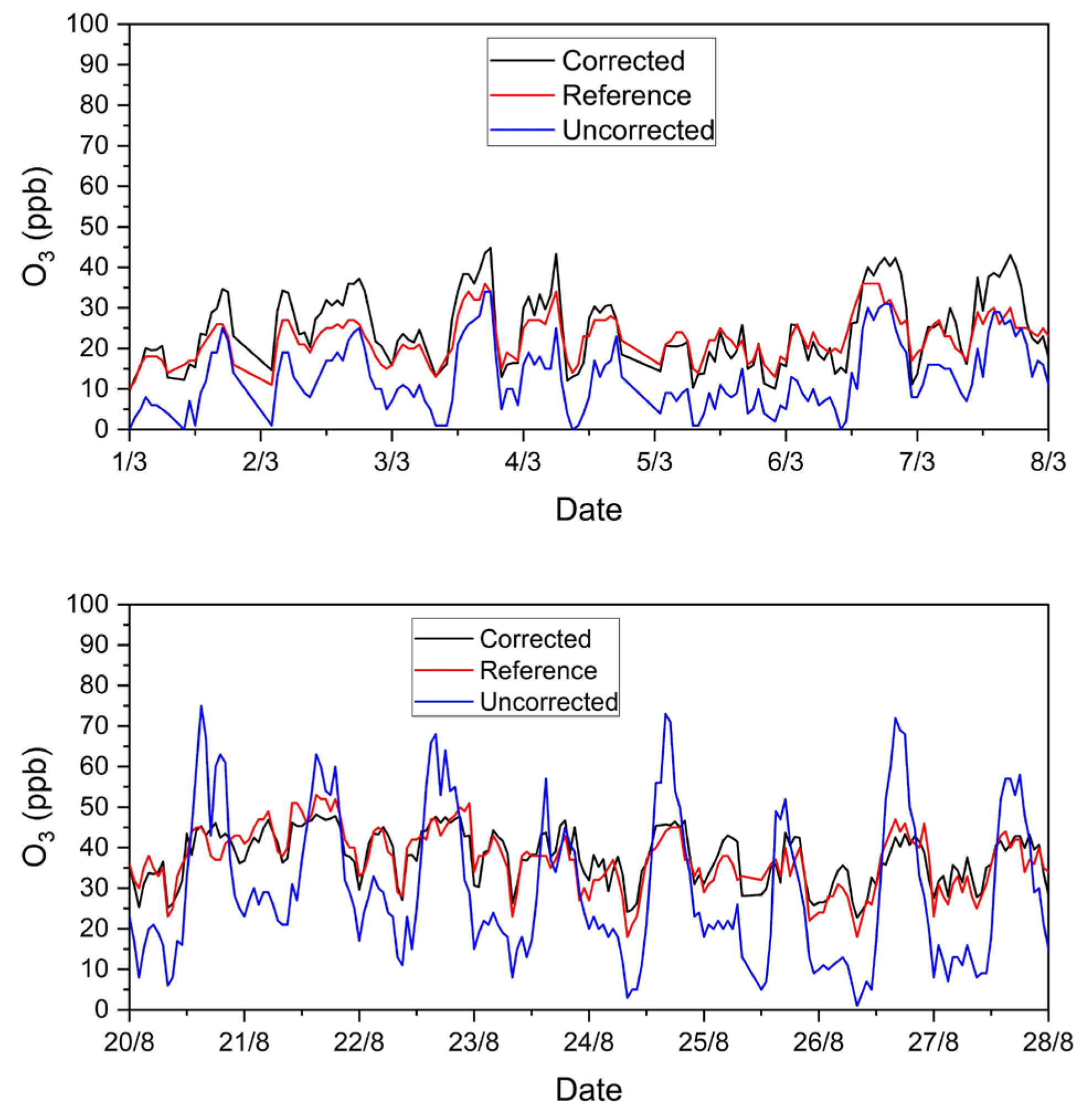
Figure 7.
Time series of O3 concentrations for two 7-day periods of the test set (2022). The uncorrected O3 low-cost sensor reading is displayed with a blue line, the RF-corrected O3 estimation is displayed with a black line, and the reference O3 concentration is displayed with a red line.
The RF algorithm performed well once more. During the training period, the ME of the predicted O3 reached 5.1 ppb, whilst it was 4.3 ppb in the test period (Table 6).
Table 6.
Agreement metrics between the reference O3 concentrations and the corrected ENSENSIA readings.
The uncorrected O3 sensor reading had a ME of 13 ppb, an R2 of 0.52, and a nME of 0.55 (Table 5). Correcting the sensor with the RF algorithm improved the performance. The corrected concentrations yielded a ME of 4.3 ppb, an R2 of 0.69, and a nME of 0.15 (Table 6).
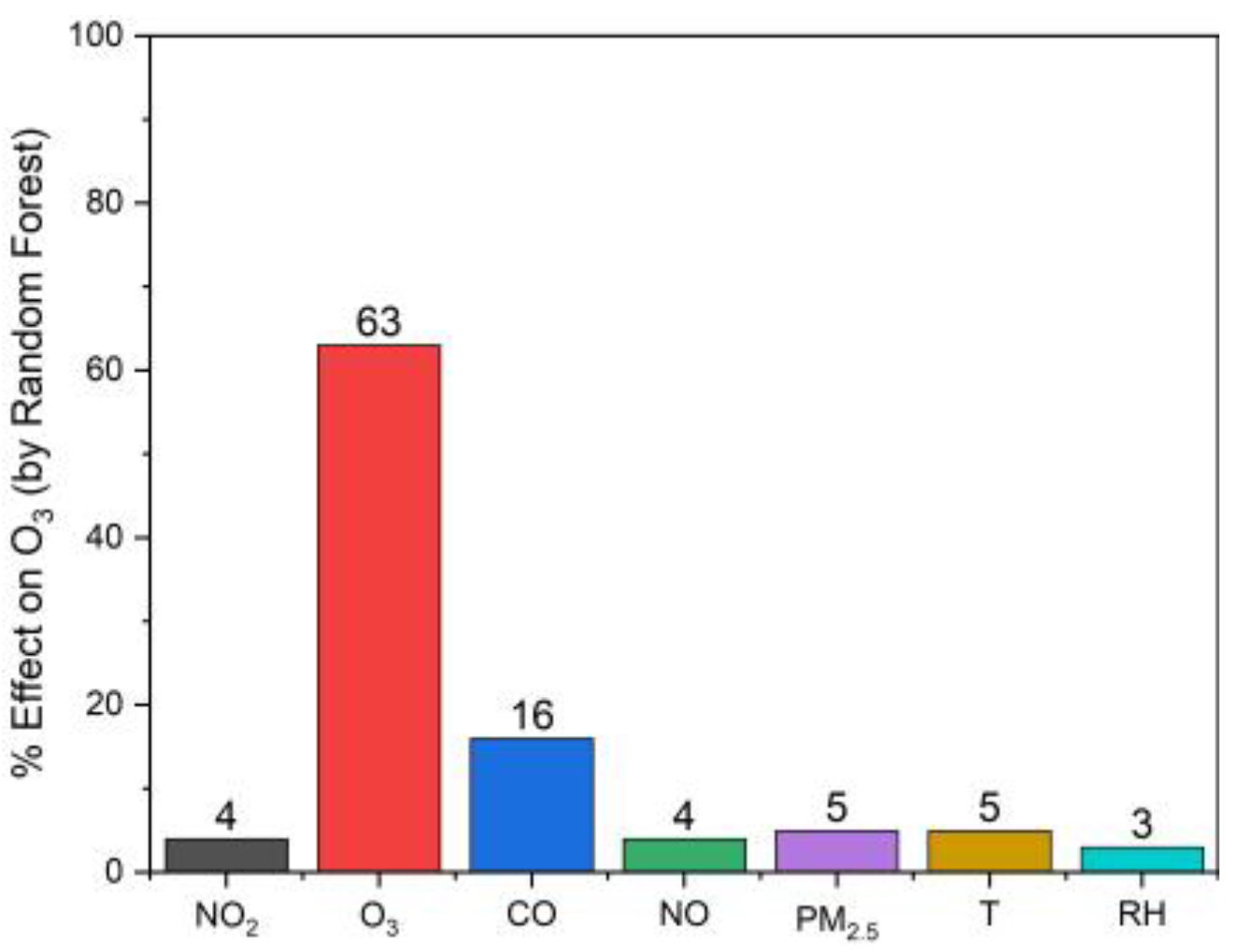
RF selects the raw reading of O3 as its most important input measurement (63% importance). The CO measurement is rated at 16%. Figure 8 illustrates the importance of each ENSENSIA reading regarding the correction of O3 by the RF algorithm.
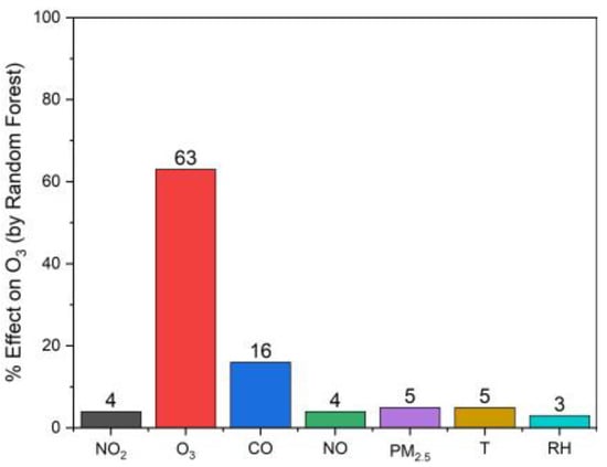
Figure 8.
The importance of the ENSENSIA readings for correcting O3 using the RF algorithm based on the training set (2021).
3.3. Comparisons with Previous Studies
The above results are in general consistent with other recent studies evaluating the same NO2 and O3 sensors in urban areas for long time-periods. Table 7 provides a summary of the results.
Table 7.
Summary of recent studies evaluating the performance of sensor correction algorithms.
4. Conclusions and Discussion
The current study employed well-established ML and DL algorithms to correct raw ENSENSIA readings. Training has been performed using one-year (2021) hourly data gathered from the ENSENSIA device and regulatory instrumentation on a city-center site. Data collected from the same site between 1 January 2022 and 30 October 2022 were used as test sets for evaluating the algorithms’ suitability in correcting unseen data from the same device and on the same site. The RF algorithm exhibited the best performance in correcting O3 and NO2. The NO2 ME was reduced from 9.4 ppb to 3 ppb, whilst R2 was improved from 0.22 to 0.86. Similar results were obtained for O3, wherein ME was reduced from 13 to 4.3 ppb and R2 increased from 0.52 to 0.69.
The study suggests utilizing all sensor readings besides the gas under examination for building the ML algorithm. Available ENSENSIA measurements included CO, NO, PM2.5, T, and RH, besides NO2 and O3. The RF revealed a cross-sensitivity between the sensors’ readings. For correcting the NO2 measurement, RF selected the raw CO and NO measurements as its top predictors (with importance of 48% and 30%, respectively), whereas the raw NO2 measurement was found to be less significant (8% importance). This fact highlights the interconnection between the mentioned sensors. In correcting O3, RF selected the initial O3 measurement as the most important attribute (with an importance of 63%), whereas the CO measurement was also significant (16%). RF graded the influence of temperature and humidity as insignificant in both cases. This may suggest that the sensors are relatively robust to T and RH variations. The observed cross-sensitivity of both sensors to other pollutants in the field was significantly higher according to RF than the one reported in the manufacturer’s datasheet.
Aging of low cost sensors can be an important problem. The OX-B431 and NO2-B43F sensors come with a two-year lifespan guarantee. After this time, drift is expected and the sensors’ sensitivity to temperature and humidity variations may change. The deployed sensors were brand-new during the training period (2021), and therefore were one-year-old during the evaluation period (2022). The NO2-B431 sensor (uncorrected) showed consistent R2 (0.22) in the two years (Table 3) compared to the reference monitor, while its ME was 0.8 ppb higher in 2022. This may be just deterioration of the sensor, but clearly additional measurements are needed to explore this issue.
There was no evidence of deterioration of the OX-B431 sensor performance in the second year. During 2021, the O3 measurements of the sensor had a ME of 13.9 ppb, a little higher than that of 13 ppb, in 2022. Similarly, R2 was 0.39 in 2021 and 0.52 in 2022. Our work suggests that training the RF with ENSENSIA data for one year is adequate to reproduce the reference concentrations of O3 and NO2 for at least one year, with significant error reduction.
Field calibration of low-cost sensors is essential to improve the sensors’ performance in ambient conditions. In this work, we presented the field calibration of the ENSENSIA device, a low-cost AQ monitoring station developed by the authors’ affiliation. This study focused on the NO2 and O3 sensors of the device and employed several state-of-the-art ML and DL methods for the calibration task. Among them, the RF algorithm was the best method for correcting the non-linear raw sensor readings. ML and DL will probably play an important role in sensor data correction tasks in the future.
Author Contributions
Conceptualization, I.D.A., G.F. and S.N.P.; methodology, I.D.A. and G.F.; writing—original draft preparation, I.D.A.; writing—review and editing, G.F. and S.N.P.; supervision, S.N.P. All authors have read and agreed to the published version of the manuscript.
Funding
This research was funded by EU Horizon Europe, project SynAirG, grant number 101057271.
Informed Consent Statement
Not applicable.
Data Availability Statement
The data of the study are available upon request by S.N.P. (spyros@chemeng.upatras.gr).
Acknowledgments
We thank the Directorate of Environment and Spatial Planning of the Region of Western Greece for the provision of data and their overall cooperation.
Conflicts of Interest
The authors declare no conflict of interest.
References
- Malings, C.; Tanzer, R.; Hauryliuk, A.; Saha, P.K.; Robinson, A.L.; Presto, A.A.; Subramanian, R. Fine particle mass monitoring with low-cost sensors: Corrections and long-term performance evaluation. Aerosol Sci. Technol. 2020, 54, 160–174. [Google Scholar] [CrossRef]
- Lelieveld, J.; Haines, A.; Pozzer, A. Age-dependent health risk from ambient air pollution: A modelling and data analysis of childhood mortality in middle-income and low-income countries. Lancet Planet. Health 2018, 2, e292–e300. [Google Scholar] [CrossRef]
- Goldemberg, J.; Martinez-Gomez, J.; Sagar, A.; Smith, K.R. Household air pollution, health, and climate change: Cleaning the air. Environ. Res. Lett. 2018, 13, 030201. [Google Scholar] [CrossRef]
- Nuvolone, D.; Petri, D.; Voller, F. The effects of ozone on human health. Environ. Sci. Pollut. Res. 2018, 25, 8074–8088. [Google Scholar] [CrossRef] [PubMed]
- Atkinson, R.W.; Butland, B.K.; Anderson, H.R.; Maynard, R.L. Long-term concentrations of nitrogen dioxide and mortality: A meta-analysis of cohort studies. Epidemiology 2018, 29, 460. [Google Scholar] [CrossRef]
- Rai, A.C.; Kumar, P.; Pilla, F.; Skouloudis, A.N.; Di Sabatino, S.; Ratti, C.; Yasar, A.; Rickerby, D. End-user perspective of low-cost sensors for outdoor air pollution monitoring. Sci. Total Environ. 2017, 607–608, 691–705. [Google Scholar] [CrossRef]
- Spinelle, L.; Gerboles, M.; Kotsev, A.; Signorini, M. Evaluation of Low-Cost Sensors for Air Pollution Monitoring: Effect of Gaseous Interfering Compounds and Meteorological Conditions; EUR 28601 EN; Publications Office of the European Union: Luxembourg, 2017. [Google Scholar] [CrossRef]
- Schneider, P.; Castell, N.; Vogt, M.; Dauge, F.R.; Lahoz, W.A.; Bartonova, A. Mapping urban air quality in near real-time using observations from low-cost sensors and model information. Environ. Int. 2017, 106, 234–247. [Google Scholar] [CrossRef]
- Kosmopoulos, G.; Salamalikis, V.; Pandis, S.N.; Yannopoulos, P.; Bloutsos, A.A.; Kazantzidis, A. Low-cost sensors for measuring airborne particulate matter: Field evaluation and calibration at a south-eastern European site. Sci. Total Environ. 2020, 748, 141396. [Google Scholar] [CrossRef] [PubMed]
- Giordano, M.R.; Malings, C.; Pandis, S.N.; Presto, A.A.; McNeill, V.F.; Westervelt, D.M.; Beekmann, M.; Subramanian, R. From low-cost sensors to high-quality data: A summary of challenges and best practices for effectively calibrating low-cost particulate matter mass sensors. J. Aerosol Sci. 2021, 158, 105833. [Google Scholar] [CrossRef]
- Zimmerman, N.; Presto, A.A.; Kumar, S.P.N.; Gu, J.; Hauryliuk, A.; Robinson, E.S.; Robinson, A.L.; Subramanian, R. A machine learning calibration model using random forests to improve sensor performance for lower-cost air quality monitoring. Atmos. Meas. Tech. 2018, 11, 291–313. [Google Scholar] [CrossRef]
- van Ratingen, S.; Vonk, J.; Blokhuis, C.; Wesseling, J.; Tielemans, E.; Weijers, E. Seasonal influence on the performance of low-cost NO2 sensor calibrations. Sensors 2021, 21, 7919. [Google Scholar] [CrossRef] [PubMed]
- Han, P.; Mei, H.; Liu, D.; Zeng, N.; Tang, X.; Wang, Y.; Pan, Y. Calibrations of low-cost air pollution monitoring sensors for CO, NO2, O3, and SO2. Sensors 2021, 21, 256. [Google Scholar] [CrossRef] [PubMed]
- Christakis, I.; Hloupis, G.; Stavrakas, I.; Tsakiridis, O. Low cost sensor implementation and evaluation for measuring NO2 and O3 pollutants. In Proceedings of the 2020 9th International Conference on Modern Circuits and Systems Technologies (MOCAST), Bremen, Germany, 7–9 September 2020; pp. 1–4. [Google Scholar]
- Margaritis, D.; Keramydas, C.; Papachristos, I.; Lambropoulou, D. Calibration of low-cost gas sensors for air quality monitoring. Aerosol Air Qual. Res. 2021, 21, 210073. [Google Scholar] [CrossRef]
- Apostolopoulos, I.D.; Fouskas, G.; Pandis, S.N. An IoT integrated air quality monitoring device based on microcomputer technology and leading industry low-cost sensor solutions. In Future Access Enablers for Ubiquitous and Intelligent Infrastructures; Perakovic, D., Knapcikova, L., Eds.; Lecture Notes of the Institute for Computer Sciences, Social Informatics and Telecommunications Engineering; Springer International Publishing: Cham, Switzerland, 2022; Volume 445, pp. 122–140. ISBN 978-3-031-15100-2. [Google Scholar]
- Mohri, M.; Rostamizadeh, A.; Talwalkar, A. Foundations of Machine Learning; MIT Press: Cambridge, MA, USA, 2018. [Google Scholar]
- Svetnik, V.; Liaw, A.; Tong, C.; Culberson, J.C.; Sheridan, R.P.; Feuston, B.P. Random forest: A classification and regression tool for compound classification and QSAR modeling. J. Chem. Inf. Comput. Sci. 2003, 43, 1947–1958. [Google Scholar] [CrossRef]
- Quinlan, J.R. Bagging, boosting, and C4.5. In Proceedings of the 13th National Conference on Artificial Intelligence, Portland, Oregon, 4–8 August 1996; Volume 1, pp. 725–730. [Google Scholar]
- Dietterich, T.G. Ensemble methods in machine learning. In Multiple Classifier Systems; Springer: Berlin/Heidelberg, Germany, 2000; pp. 1–15. [Google Scholar]
- Hochreiter, S.; Schmidhuber, J. Long short-term memory. Neural Comput. 1997, 9, 1735–1780. [Google Scholar] [CrossRef] [PubMed]
- Sherstinsky, A. Fundamentals of Recurrent Neural Network (RNN) and Long Short-Term Memory (LSTM) network. Phys. D Nonlinear Phenom. 2020, 404, 132306. [Google Scholar] [CrossRef]
- LeCun, Y.; Bengio, Y.; Hinton, G. Deep learning. Nature 2015, 521, 436–444. [Google Scholar] [CrossRef] [PubMed]
- Gu, J.; Wang, Z.; Kuen, J.; Ma, L.; Shahroudy, A.; Shuai, B.; Liu, T.; Wang, X.; Wang, G.; Cai, J.; et al. Recent advances in convolutional neural networks. Pattern Recognit. 2018, 77, 354–377. [Google Scholar] [CrossRef]
- Borrego, C.; Ginja, J.; Coutinho, M.; Ribeiro, C.; Karatzas, K.; Sioumis, T.; Katsifarakis, N.; Konstantinidis, K.; De Vito, S.; Esposito, E.; et al. Assessment of air quality microsensors versus reference methods: The EuNetAir Joint Exercise—Part II. Atmos. Environ. 2018, 193, 127–142. [Google Scholar] [CrossRef]
- Castell, N.; Dauge, F.R.; Schneider, P.; Vogt, M.; Lerner, U.; Fishbain, B.; Broday, D.; Bartonova, A. Can commercial low-cost sensor platforms contribute to air quality monitoring and exposure estimates? Environ. Int. 2017, 99, 293–302. [Google Scholar] [CrossRef] [PubMed]
- Zauli-Sajani, S.; Marchesi, S.; Pironi, C.; Barbieri, C.; Poluzzi, V.; Colacci, A. Assessment of air quality sensor system performance after relocation. Atmos. Pollut. Res. 2021, 12, 282–291. [Google Scholar] [CrossRef]
Disclaimer/Publisher’s Note: The statements, opinions and data contained in all publications are solely those of the individual author(s) and contributor(s) and not of MDPI and/or the editor(s). MDPI and/or the editor(s) disclaim responsibility for any injury to people or property resulting from any ideas, methods, instructions or products referred to in the content. |
© 2023 by the authors. Licensee MDPI, Basel, Switzerland. This article is an open access article distributed under the terms and conditions of the Creative Commons Attribution (CC BY) license (https://creativecommons.org/licenses/by/4.0/).