
Spatiotemporal Air Pollution Forecasting in Houston-TX: A Case Study for Ozone Using Deep Graph Neural Networks

 ,
,  ,
,  ,
, 

Abstract
1. Introduction
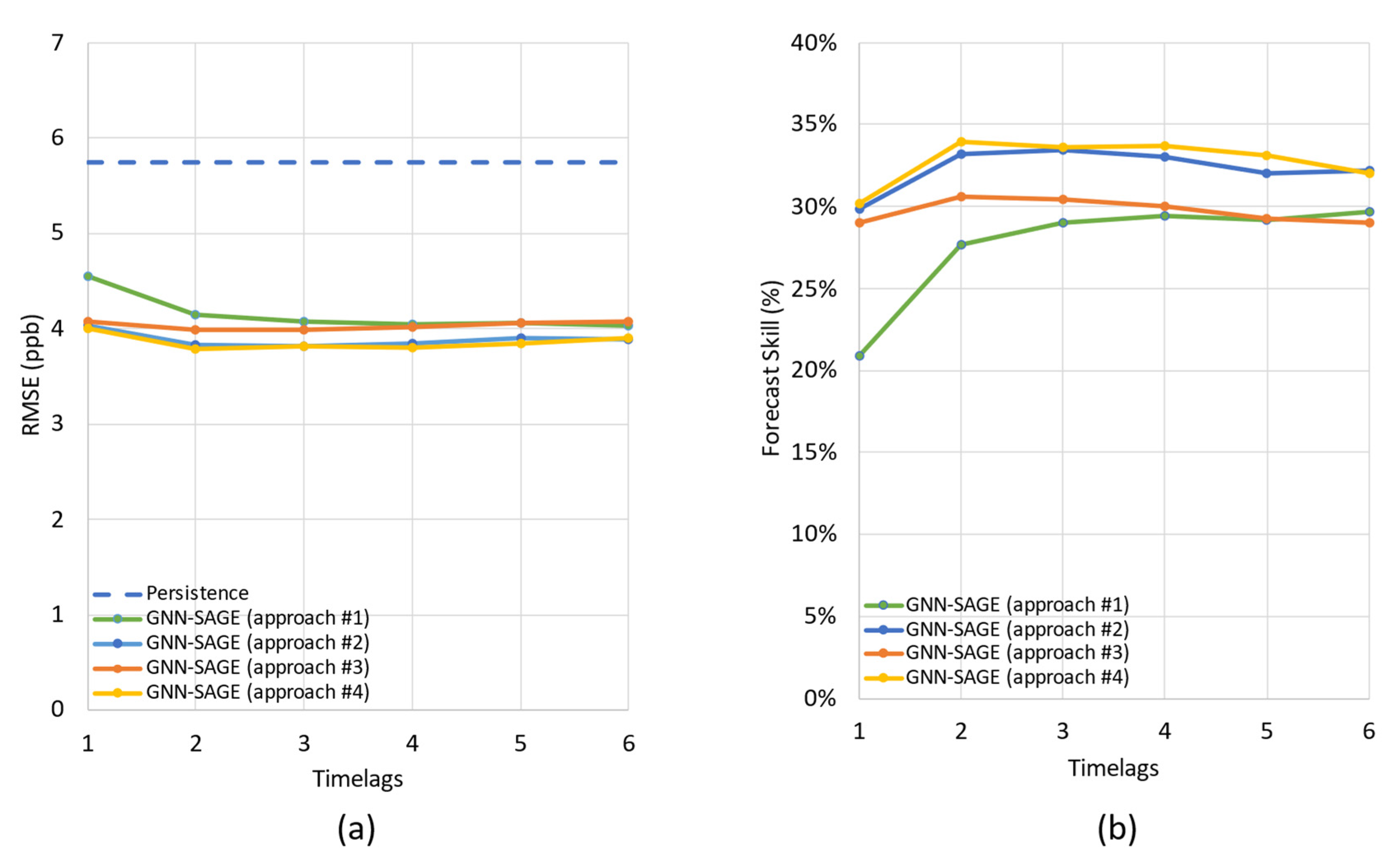
- In the first approach, the input data consisting only of past ozone concentration data and hour of the day (HoD) and day of the year (DoY) were used to estimate ozone concentration. This limitation yields the highest number of available stations to spatially feed the model.
- For the second approach, ozone, NO2/NOX and weather information (wind speed, wind direction, outdoor temperature, relative humidity, solar radiation) and HoD/DoY were used to estimate ozone concentration. This is the maximum weather data that we can use, which yields a smaller number of stations but favours some important ozone precursors (chemical and physical).
- The third approach used past ozone data, NO2/NOX, Volatile organic compounds (VOCs) (propane, isobutane, benzene, toluene, ethylbenzene), weather (wind speed, wind direction, outdoor temperature) and HoD/DoY information to estimate ozone concentration. The VOCs information limited the other input variables and the number of stations, resulting in the smallest set of stations.
- Finally, the last approach used past ozone data, NO2/NOX, weather and HoD/DoY information, aiming for the maximum number of stations aggregated with chemical/physical information.
- Developing a new model to forecast air pollution concentrations.
- Analyzing the inclusion of spatial information to deep learning air quality forecasts.
- The importance analysis of input variables for different data configurations over distinct deep learning forecasting horizons.
- Producing an accurate and reliable model for ozone prediction based on DL and graph theory.
2. Materials and Methods
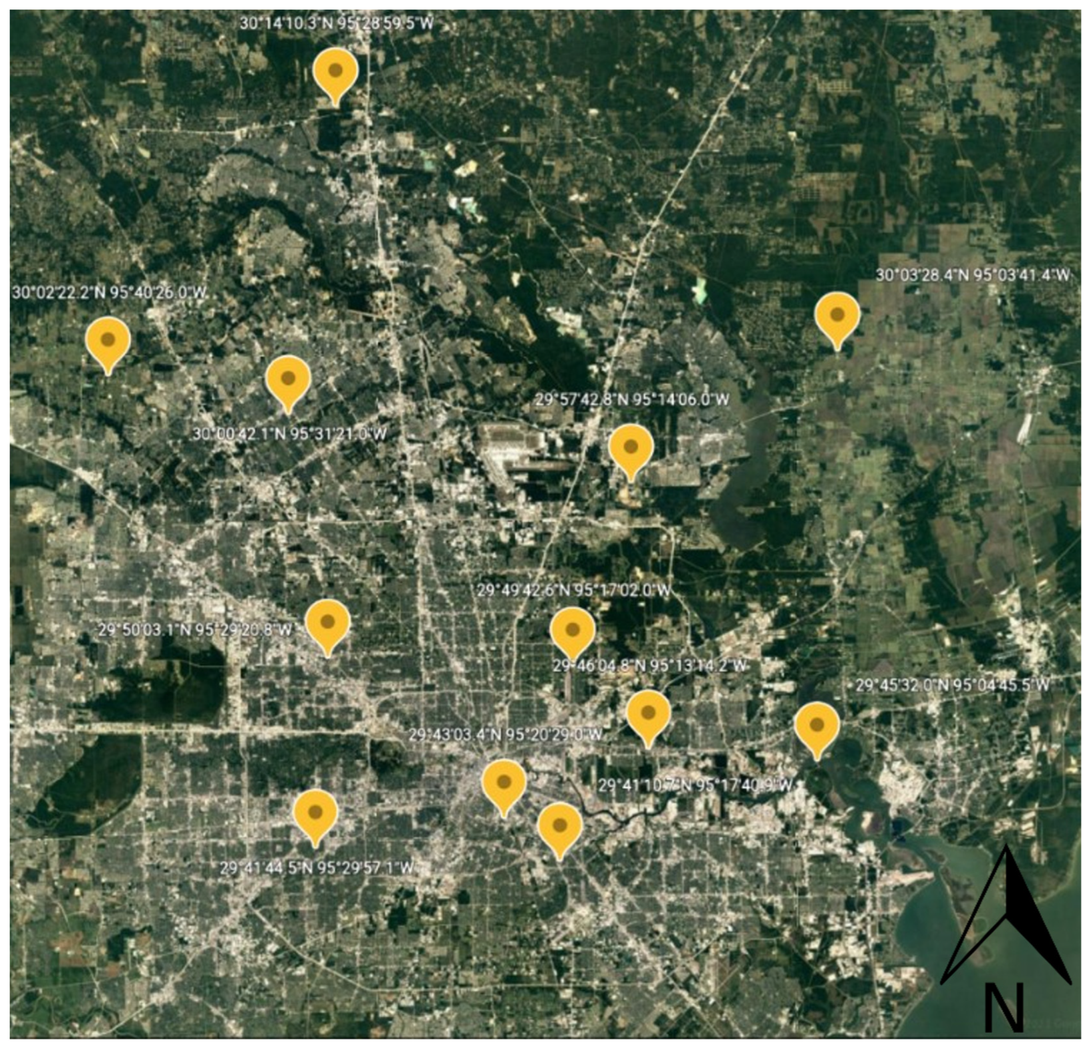
2.1. Houston Database
2.2. Persistence Model
2.3. LASSO Model
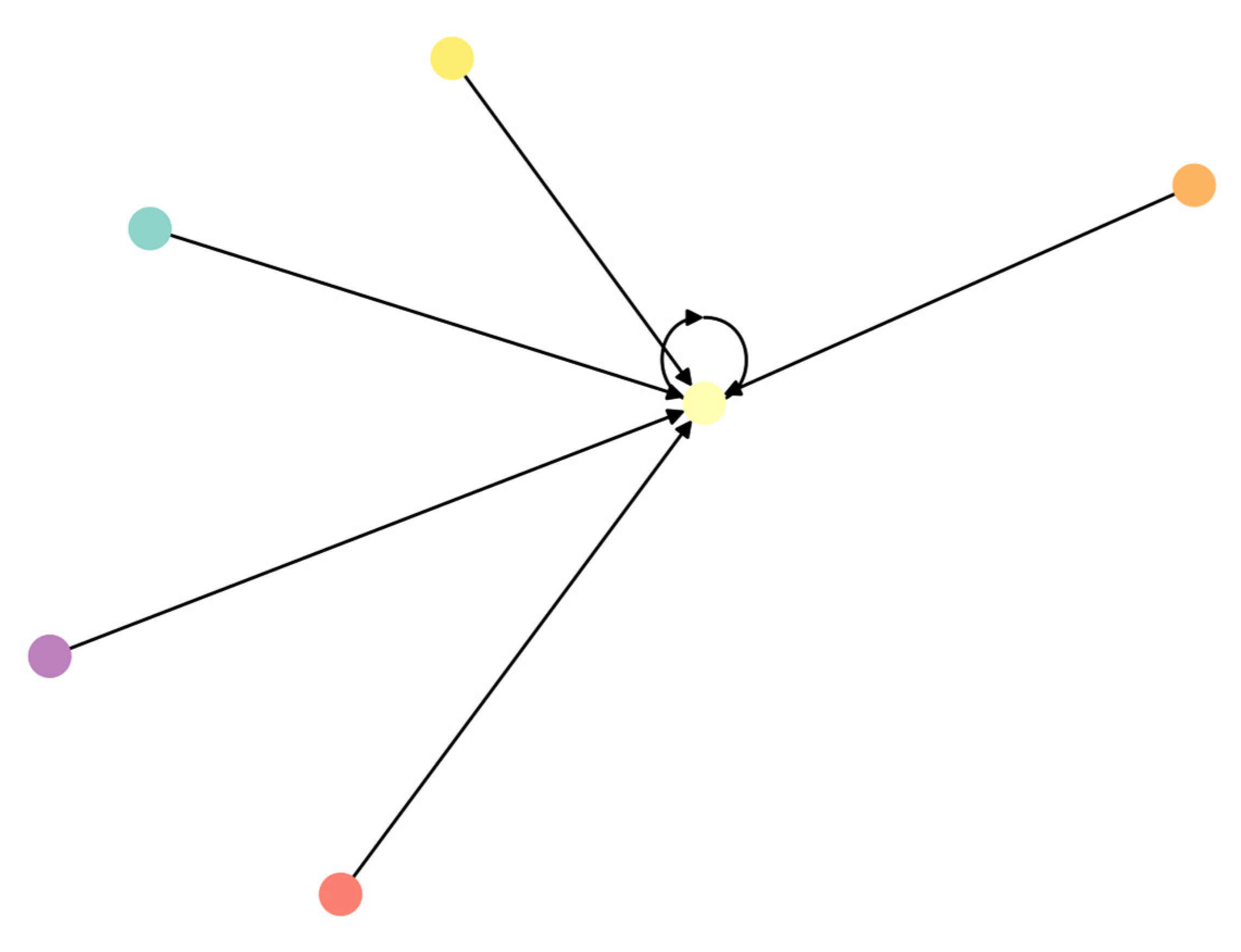
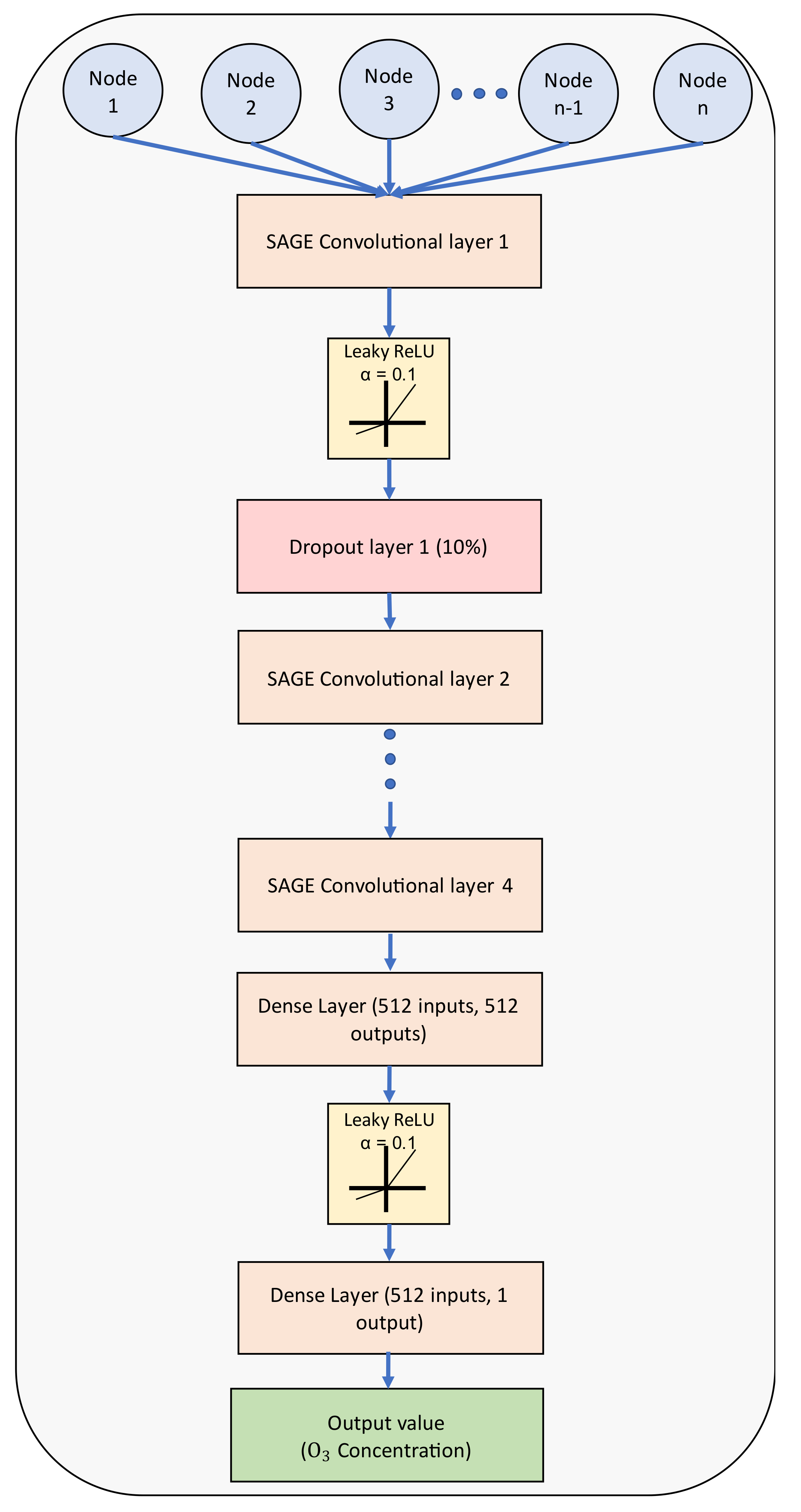
2.4. GraphSAGE Model
2.5. Evaluation Metrics
2.6. SHAP Analysis
3. Results
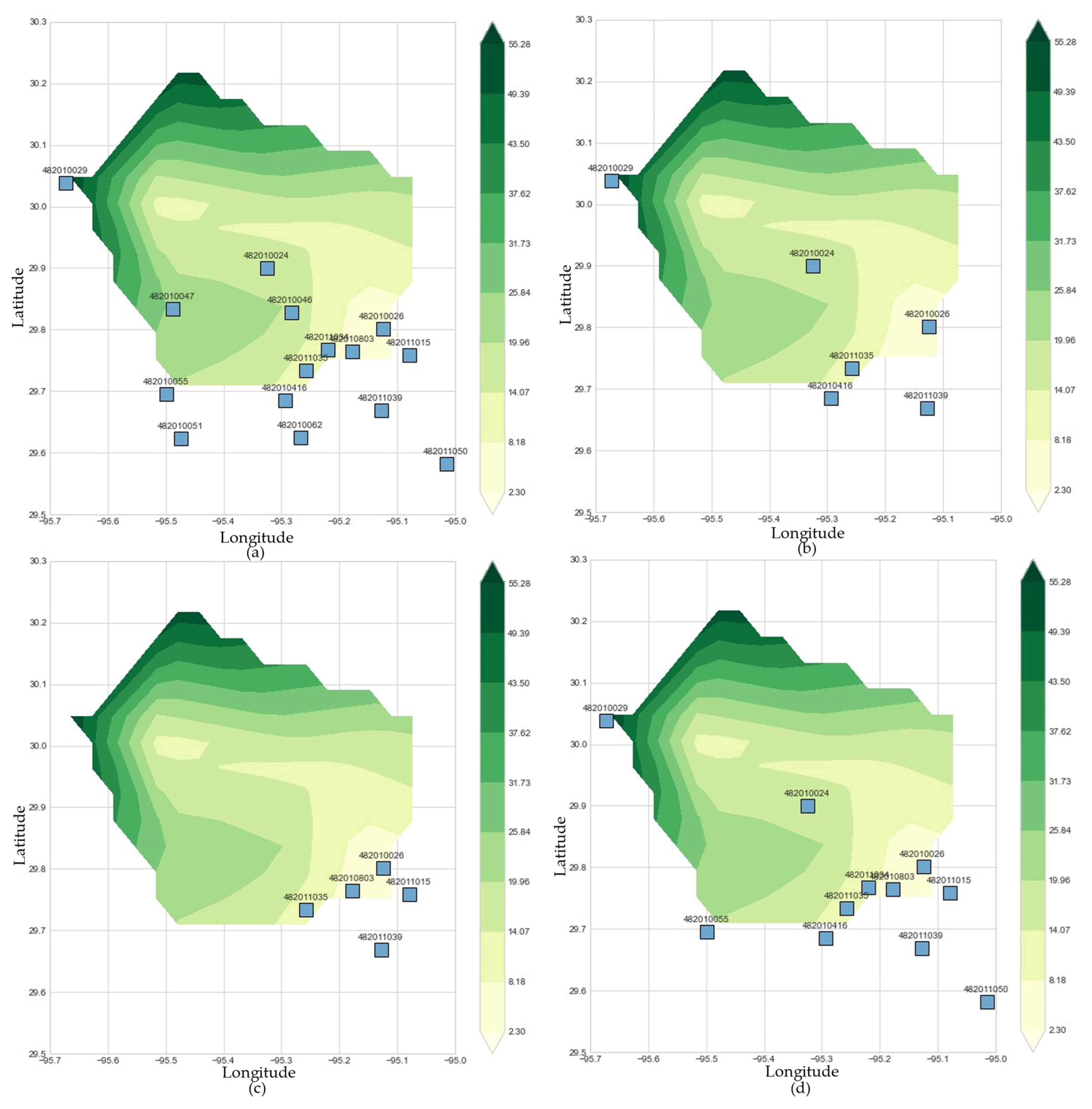
3.1. Dataset Size
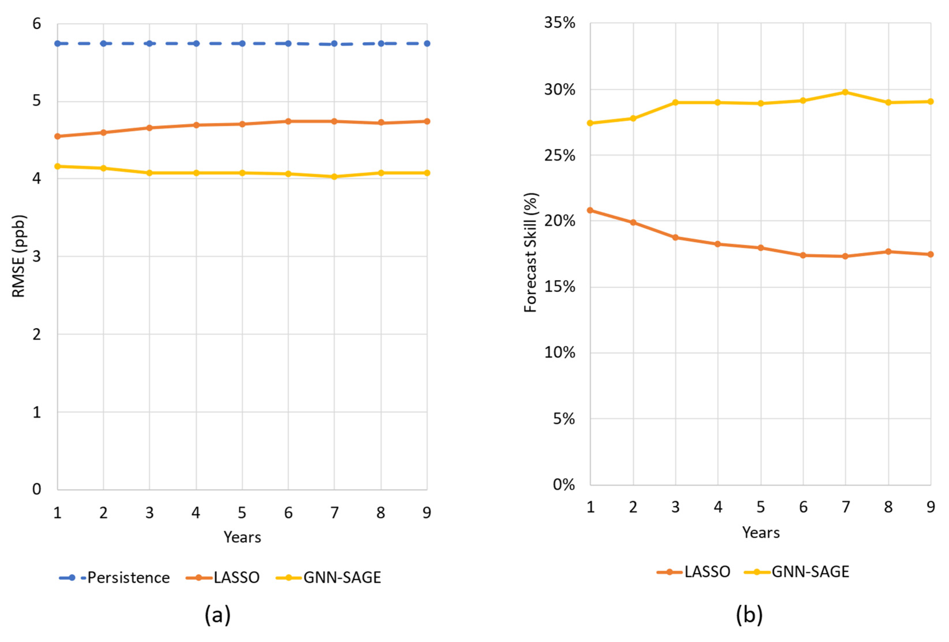
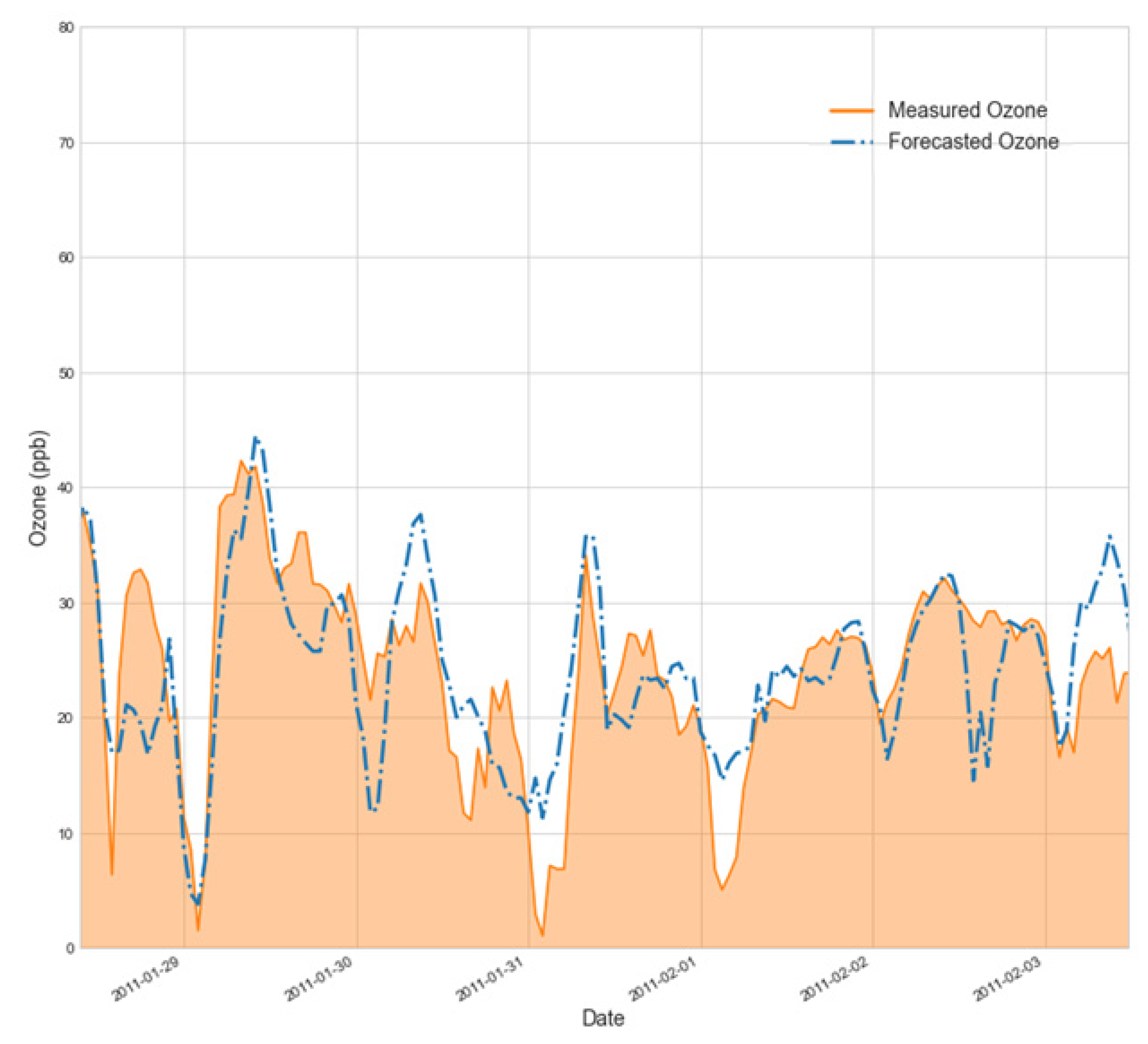
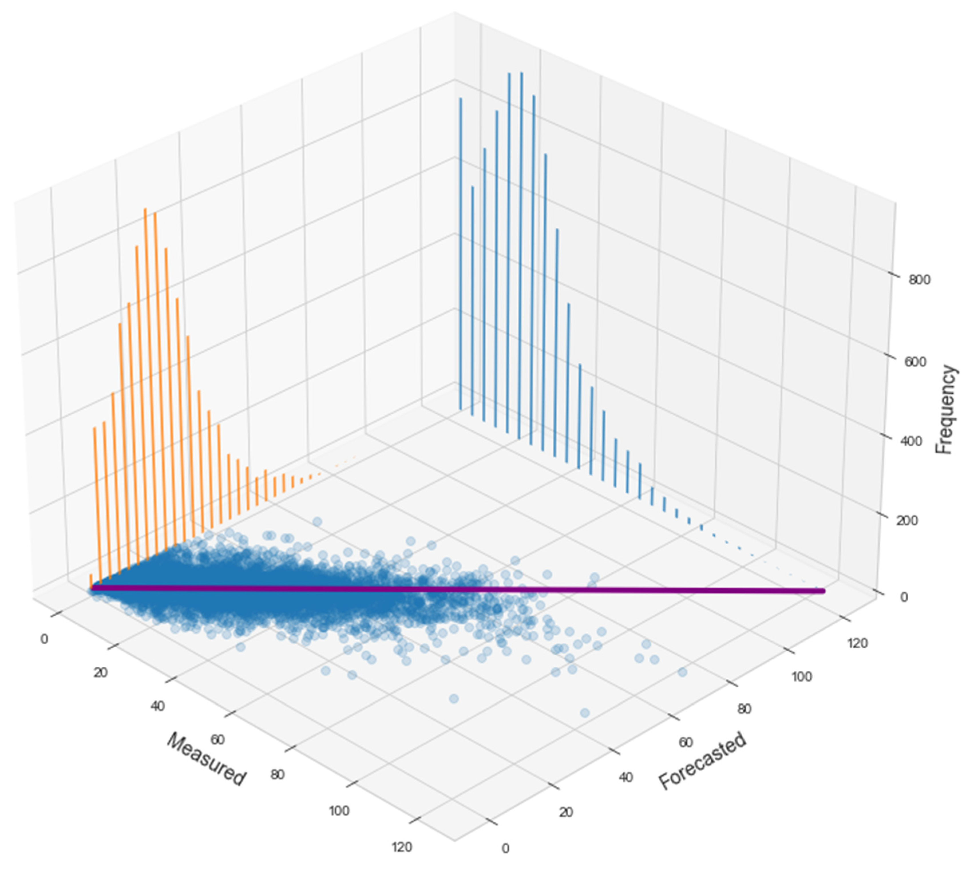
3.2. Ozone Concentration Prediction for 1 h Forecast Horizon
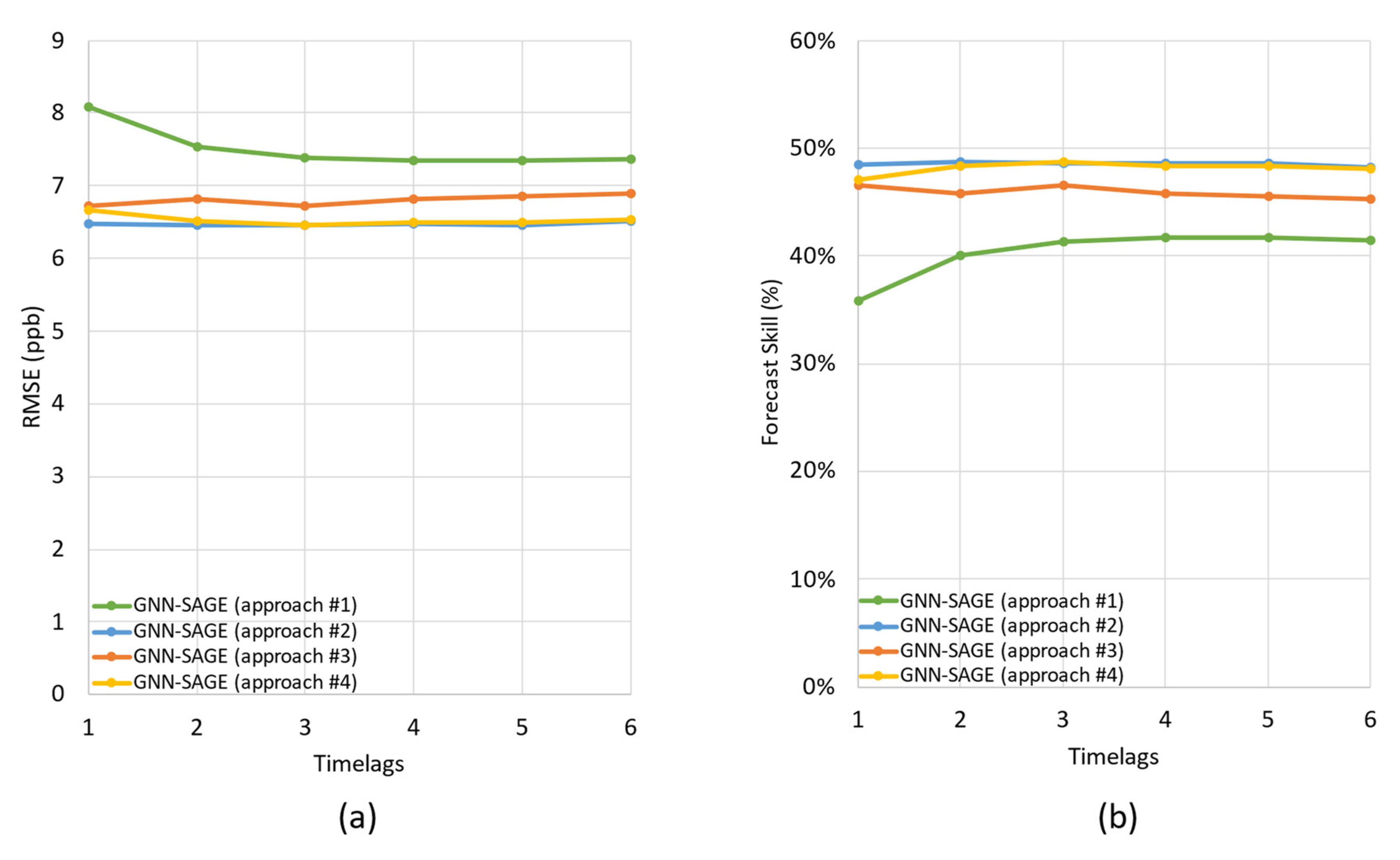
3.3. Ozone Concentration Prediction for 3 h Forecast Horizon
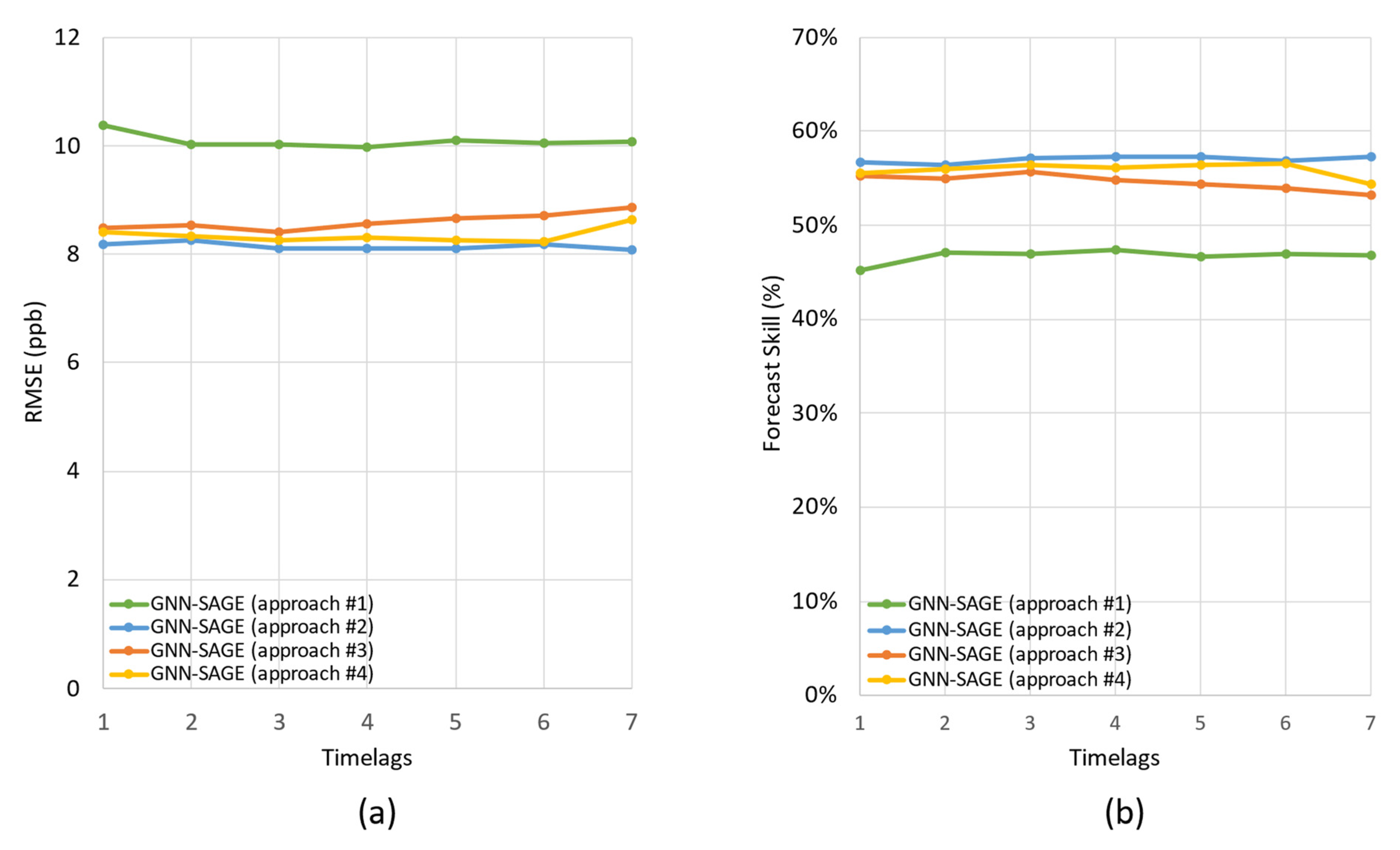
3.4. Ozone Concentration Prediction for 6 h Forecast Horizon
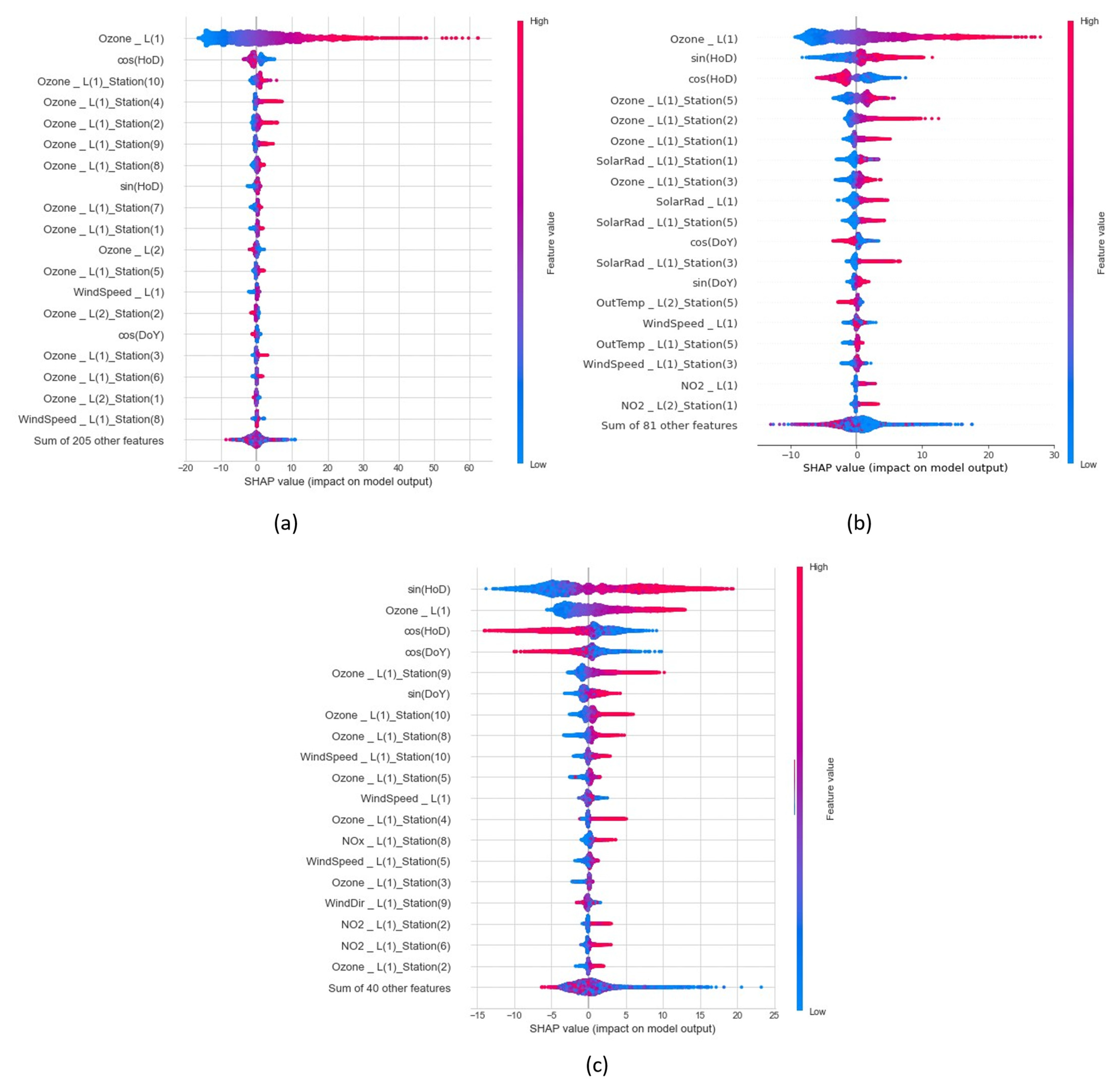
3.5. Importance of Different Input Attributes to Ozone Forecasting
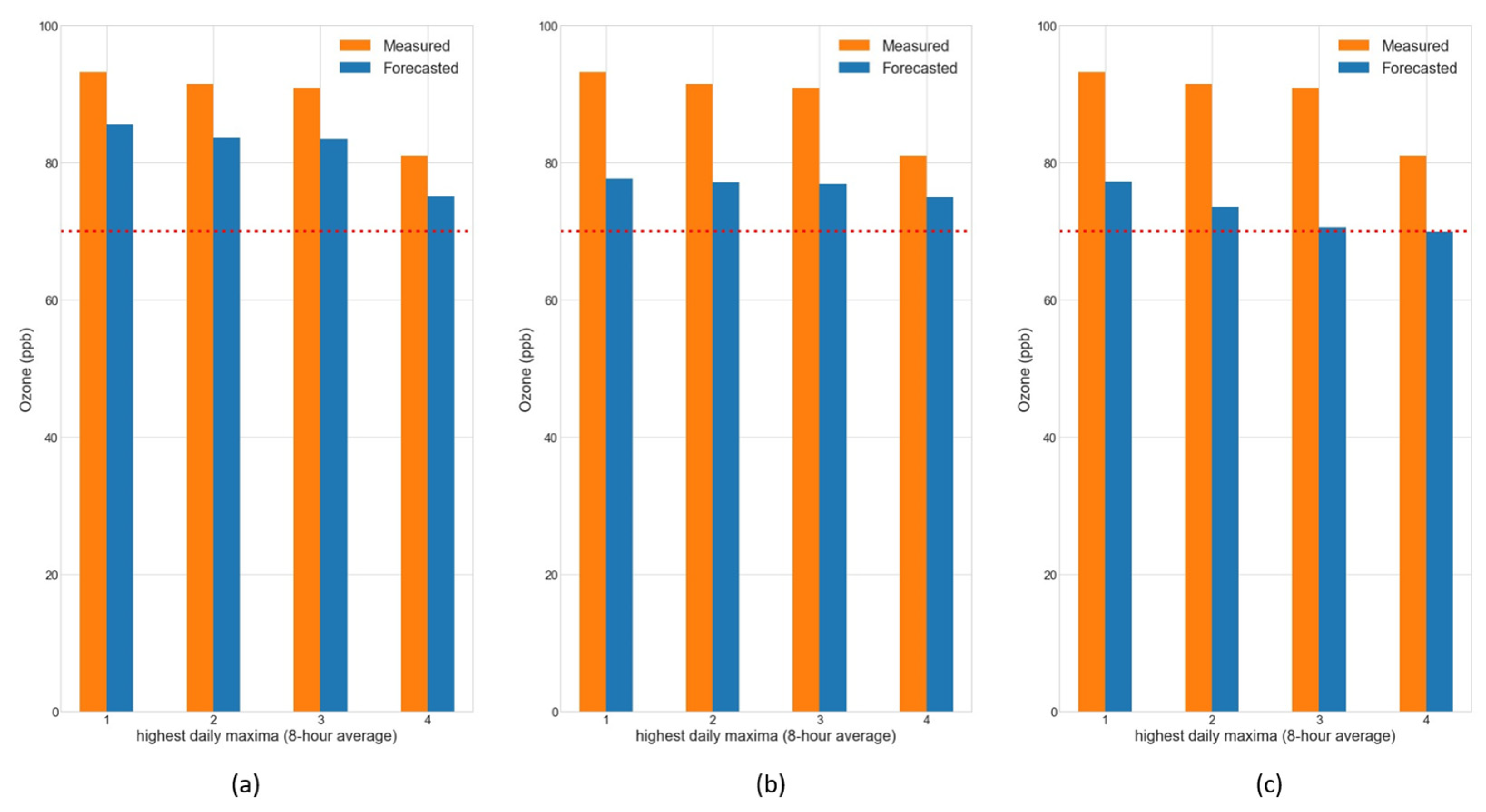
3.6. Model’s Performance for the Determination of Compliance with EPA Regulations
4. Discussion
5. Conclusions
Author Contributions
Funding
Institutional Review Board Statement
Informed Consent Statement
Data Availability Statement
Conflicts of Interest
References
- Wang, Z.; Li, G.; Huang, J.; Wang, Z.; Pan, X. Impact of Air Pollution Waves on the Burden of Stroke in a Megacity in China. Atmos. Environ. 2019, 202, 142–148. [Google Scholar] [CrossRef]
- Statistical Review of World Energy—Energy Economics—Home. Available online: https://www.bp.com/en/global/corporate/energy-economics/statistical-review-of-world-energy.html (accessed on 7 December 2022).
- Croze, M.L.; Zimmer, L. Ozone Atmospheric Pollution and Alzheimer’s Disease: From Epidemiological Facts to Molecular Mechanisms. JAD 2018, 62, 503–522. [Google Scholar] [CrossRef] [PubMed]
- Lin, C.-C.; Chiu, C.-C.; Lee, P.-Y.; Chen, K.-J.; He, C.-X.; Hsu, S.-K.; Cheng, K.-C. The Adverse Effects of Air Pollution on the Eye: A Review. Int. J. Environ. Res. Public Health 2022, 19, 1186. [Google Scholar] [CrossRef]
- Sivarethinamohan, R. Impact of Air Pollution in Health and Socio-Economic Aspects: Review on Future Approach. Mater. Today Proc. 2021, 37, 2725–2729. [Google Scholar] [CrossRef]
- Li, G.; Lu, H.; Hu, W.; Liu, J.; Hu, M.; He, J.; Huang, F. Outdoor Air Pollution Enhanced the Association between Indoor Air Pollution Exposure and Hypertension in Rural Areas of Eastern China. Env. Sci. Pollut. Res. 2022, 29, 74909–74920. [Google Scholar] [CrossRef]
- Nazar, W.; Niedoszytko, M. Air Pollution in Poland: A 2022 Narrative Review with Focus on Respiratory Diseases. Int. J. Environ. Res. Public Health 2022, 19, 895. [Google Scholar] [CrossRef]
- Tian, X.; Zhang, C.; Xu, B. The Impact of Air Pollution on Residents’ Happiness: A Study on the Moderating Effect Based on Pollution Sensitivity. Int. J. Environ. Res. Public Health 2022, 19, 7536. [Google Scholar] [CrossRef]
- Vohra, K.; Vodonos, A.; Schwartz, J.; Marais, E.A.; Sulprizio, M.P.; Mickley, L.J. Global Mortality from Outdoor Fine Particle Pollution Generated by Fossil Fuel Combustion: Results from GEOS-Chem. Environ. Res. 2021, 195, 110754. [Google Scholar] [CrossRef]
- Huang, J.; Pan, X.; Guo, X.; Li, G. Impacts of Air Pollution Wave on Years of Life Lost: A Crucial Way to Communicate the Health Risks of Air Pollution to the Public. Environ. Int. 2018, 113, 42–49. [Google Scholar] [CrossRef]
- Lelieveld, J.; Evans, J.S.; Fnais, M.; Giannadaki, D.; Pozzer, A. The Contribution of Outdoor Air Pollution Sources to Premature Mortality on a Global Scale. Nature 2015, 525, 367–371. [Google Scholar] [CrossRef]
- Perera, F.; Nadeau, K. Climate Change, Fossil-Fuel Pollution, and Children’s Health. N. Engl. J. Med. 2022, 386, 2303–2314. [Google Scholar] [CrossRef]
- Balogun, A.-L.; Tella, A.; Baloo, L.; Adebisi, N. A Review of the Inter-Correlation of Climate Change, Air Pollution and Urban Sustainability Using Novel Machine Learning Algorithms and Spatial Information Science. Urban Clim. 2021, 40, 100989. [Google Scholar] [CrossRef]
- IPCC. Global Warming of 1.5 °C: IPCC Special Report on Impacts of Global Warming of 1.5 °C above Pre-Industrial Levels in Context of Strengthening Response to Climate Change, Sustainable Development, and Efforts to Eradicate Poverty, 1st ed.; Cambridge University Press: Cambridge, UK, 2022; ISBN 978-1-00-915794-0. [Google Scholar]
- Li, Y.; Shang, J.; Zhang, C.; Zhang, W.; Niu, L.; Wang, L.; Zhang, H. The Role of Freshwater Eutrophication in Greenhouse Gas Emissions: A Review. Sci. Total Environ. 2021, 768, 144582. [Google Scholar] [CrossRef]
- Mikhaylov, A.; Moiseev, N.; Aleshin, K.; Burkhardt, T. Global Climate Change and Greenhouse Effect. Entrep. Sustain. Issues 2020, 7, 2897–2913. [Google Scholar] [CrossRef]
- Fisher, S.; Bellinger, D.C.; Cropper, M.L.; Kumar, P.; Binagwaho, A.; Koudenoukpo, J.B.; Park, Y.; Taghian, G.; Landrigan, P.J. Air Pollution and Development in Africa: Impacts on Health, the Economy, and Human Capital. Lancet Planet. Health 2021, 5, e681–e688. [Google Scholar] [CrossRef]
- Errigo, I.M.; Abbott, B.W.; Mendoza, D.L.; Mitchell, L.; Sayedi, S.S.; Glenn, J.; Kelly, K.E.; Beard, J.D.; Bratsman, S.; Carter, T.; et al. Human Health and Economic Costs of Air Pollution in Utah: An Expert Assessment. Atmosphere 2020, 11, 1238. [Google Scholar] [CrossRef]
- Jakubowska, A.; Rabe, M. Air Pollution and Limitations in Health: Identification of Inequalities in the Burdens of the Economies of the “Old” and “New” EU. Energies 2022, 15, 6225. [Google Scholar] [CrossRef]
- Dechezleprêtre, A.; Rivers, N.; Stadler, B. The Economic Cost of Air Pollution: Evidence from Europe; OECD Economics Department Working Papers: Paris, France, 2019; Volume 1584. [Google Scholar]
- Pandey, A.; Brauer, M.; Cropper, M.L.; Balakrishnan, K.; Mathur, P.; Dey, S.; Turkgulu, B.; Kumar, G.A.; Khare, M.; Beig, G.; et al. Health and Economic Impact of Air Pollution in the States of India: The Global Burden of Disease Study. Lancet Planet Health 2021, 5, e25–e38. [Google Scholar] [CrossRef]
- Chen, Z.; Wang, F.; Liu, B.; Zhang, B. Short-Term and Long-Term Impacts of Air Pollution Control on China’s Economy. Environ. Manag. 2022, 70, 536–547. [Google Scholar] [CrossRef]
- Steinebach, Y. Instrument Choice, Implementation Structures, and the Effectiveness of Environmental Policies: A Cross-National Analysis. Regul. Gov. 2022, 16, 225–242. [Google Scholar] [CrossRef]
- Senthilkumar, N.; Gilfether, M.; Metcalf, F.; Russell, A.G.; Mulholland, J.A.; Chang, H.H. Application of a Fusion Method for Gas and Particle Air Pollutants between Observational Data and Chemical Transport Model Simulations Over the Contiguous United States for 2005. Int. J. Environ. Res. Public Health 2019, 16, 3314. [Google Scholar] [CrossRef] [PubMed]
- Liu, H.; Yan, G.; Duan, Z.; Chen, C. Intelligent Modeling Strategies for Forecasting Air Quality Time Series: A Review. Appl. Soft Comput. 2021, 102, 106957. [Google Scholar] [CrossRef]
- Wang, L.; Zhao, Y.; Shi, J.; Ma, J.; Liu, X.; Han, D.; Gao, H.; Huang, T. Predicting Ozone Formation in Petrochemical Industrialized Lanzhou City by Interpretable Ensemble Machine Learning. Environ. Pollut. 2023, 318, 120798. [Google Scholar] [CrossRef] [PubMed]
- Friberg, M.D.; Zhai, X.; Holmes, H.A.; Chang, H.H.; Strickland, M.J.; Sarnat, S.E.; Tolbert, P.E.; Russell, A.G.; Mulholland, J.A. Method for Fusing Observational Data and Chemical Transport Model Simulations To Estimate Spatiotemporally Resolved Ambient Air Pollution. Environ. Sci. Technol. 2016, 50, 3695–3705. [Google Scholar] [CrossRef] [PubMed]
- Sayeed, A.; Choi, Y.; Jung, J.; Lops, Y.; Eslami, E.; Salman, A.K. A Deep Convolutional Neural Network Model for Improving WRF Simulations. IEEE Trans. Neural Netw. Learn. Syst. 2021, 1–11. [Google Scholar] [CrossRef]
- Ballesteros-González, K.; Sullivan, A.P.; Morales-Betancourt, R. Estimating the Air Quality and Health Impacts of Biomass Burning in Northern South America Using a Chemical Transport Model. Sci. Total Environ. 2020, 739, 139755. [Google Scholar] [CrossRef]
- López-Noreña, A.I.; Berná, L.; Tames, M.F.; Millán, E.N.; Puliafito, S.E.; Fernandez, R.P. Influence of Emission Inventory Resolution on the Modeled Spatio-Temporal Distribution of Air Pollutants in Buenos Aires, Argentina, Using WRF-Chem. Atmos. Environ. 2022, 269, 118839. [Google Scholar] [CrossRef]
- Mazzeo, A.; Zhong, J.; Hood, C.; Smith, S.; Stocker, J.; Cai, X.; Bloss, W.J. Modelling the Impact of National vs. Local Emission Reduction on PM2.5 in the West Midlands, UK Using WRF-CMAQ. Atmosphere 2022, 13, 377. [Google Scholar] [CrossRef]
- Sayeed, A.; Lops, Y.; Choi, Y.; Jung, J.; Salman, A.K. Bias Correcting and Extending the PM Forecast by CMAQ up to 7 Days Using Deep Convolutional Neural Networks. Atmos. Environ. 2021, 253, 118376. [Google Scholar] [CrossRef]
- Cabaneros, S.M.; Calautit, J.K.; Hughes, B.R. A Review of Artificial Neural Network Models for Ambient Air Pollution Prediction. Environ. Model. Softw. 2019, 119, 285–304. [Google Scholar] [CrossRef]
- Kašpar, V.; Zapletal, M.; Samec, P.; Komárek, J.; Bílek, J.; Juráň, S. Unmanned Aerial Systems for Modelling Air Pollution Removal by Urban Greenery. Urban For. Urban Green. 2022, 78, 127757. [Google Scholar] [CrossRef]
- Tian, C.; Niu, T.; Wei, W. Developing a Wind Power Forecasting System Based on Deep Learning with Attention Mechanism. Energy 2022, 257, 124750. [Google Scholar] [CrossRef]
- Rocha, P.A.C.; Santos, V.O. Global Horizontal and Direct Normal Solar Irradiance Modeling by the Machine Learning Methods XGBoost and Deep Neural Networks with CNN-LSTM Layers: A Case Study Using the GOES-16 Satellite Imagery. Int. J. Energy Environ. Eng. 2022, 13, 1271–1286. [Google Scholar] [CrossRef]
- O’Donncha, F.; Hu, Y.; Palmes, P.; Burke, M.; Filgueira, R.; Grant, J. A Spatio-Temporal LSTM Model to Forecast across Multiple Temporal and Spatial Scales. Ecol. Inform. 2022, 69, 101687. [Google Scholar] [CrossRef]
- Bashir Shaban, K.; Kadri, A.; Rezk, E. Urban Air Pollution Monitoring System With Forecasting Models. IEEE Sens. J. 2016, 16, 2598–2606. [Google Scholar] [CrossRef]
- Zhan, Y.; Luo, Y.; Deng, X.; Grieneisen, M.L.; Zhang, M.; Di, B. Spatiotemporal Prediction of Daily Ambient Ozone Levels across China Using Random Forest for Human Exposure Assessment. Environ. Pollut. 2018, 233, 464–473. [Google Scholar] [CrossRef]
- Juarez, E.K.; Petersen, M.R. A Comparison of Machine Learning Methods to Forecast Tropospheric Ozone Levels in Delhi. Atmosphere 2021, 13, 46. [Google Scholar] [CrossRef]
- Seng, D.; Zhang, Q.; Zhang, X.; Chen, G.; Chen, X. Spatiotemporal Prediction of Air Quality Based on LSTM Neural Network. Alex. Eng. J. 2021, 60, 2021–2032. [Google Scholar] [CrossRef]
- Zhu, S.; Xu, J.; Zeng, J.; Yu, C.; Wang, Y.; Yan, H. Satellite-Derived Estimates of Surface Ozone by LESO: Extended Application and Performance Evaluation. Int. J. Appl. Earth Obs. Geoinf. 2022, 113, 103008. [Google Scholar] [CrossRef]
- Gilik, A.; Ogrenci, A.S.; Ozmen, A. Air Quality Prediction Using CNN+LSTM-Based Hybrid Deep Learning Architecture. Env. Sci. Pollut. Res. 2022, 29, 11920–11938. [Google Scholar] [CrossRef]
- Veličković, P.; Cucurull, G.; Casanova, A.; Romero, A.; Liò, P.; Bengio, Y. Graph Attention Networks. In Proceedings of the International Conference on Learning (ICLR), Vancouver, BC, Canada, 30 April–3 May 2018. [Google Scholar]
- Zhang, K.; Yang, X.; Cao, H.; Thé, J.; Tan, Z.; Yu, H. Multi-Step Forecast of PM2.5 and PM10 Concentrations Using Convolutional Neural Network Integrated with Spatial–Temporal Attention and Residual Learning. Environ. Int. 2023, 171, 107691. [Google Scholar] [CrossRef] [PubMed]
- Wilson, T.; Tan, P.-N.; Luo, L. A Low Rank Weighted Graph Convolutional Approach to Weather Prediction. In Proceedings of the 2018 IEEE International Conference on Data Mining (ICDM), Singapore, 17–20 November 2018; pp. 627–636. [Google Scholar]
- Zhang, S.; Tong, H.; Xu, J.; Maciejewski, R. Graph Convolutional Networks: A Comprehensive Review. Comput. Soc. Netw. 2019, 6, 11. [Google Scholar] [CrossRef]
- Qi, Y.; Li, Q.; Karimian, H.; Liu, D. A Hybrid Model for Spatiotemporal Forecasting of PM2.5 Based on Graph Convolutional Neural Network and Long Short-Term Memory. Sci. Total Environ. 2019, 664, 1–10. [Google Scholar] [CrossRef] [PubMed]
- Mao, W.; Jiao, L.; Wang, W. Long Time Series Ozone Prediction in China: A Novel Dynamic Spatiotemporal Deep Learning Approach. Build. Environ. 2022, 218, 109087. [Google Scholar] [CrossRef]
- Wang, S.; Qiao, L.; Fang, W.; Jing, G.; Sheng, V.; Zhang, Y. Air Pollution Prediction Via Graph Attention Network and Gated Recurrent Unit. Comput. Mater. Contin. 2022, 73, 673–687. [Google Scholar] [CrossRef]
- Hamilton, W.L.; Ying, R.; Leskovec, J. Inductive Representation Learning on Large Graphs. In Proceedings of the 31st International Conference on Neural Information Processing Systems (NIPS), Long Beach, CA, USA, 4–9 December 2018; pp. 1024–1034. [Google Scholar]
- Pan, S.; Roy, A.; Choi, Y.; Eslami, E.; Thomas, S.; Jiang, X.; Gao, H.O. Potential Impacts of Electric Vehicles on Air Quality and Health Endpoints in the Greater Houston Area in 2040. Atmos. Environ. 2019, 207, 38–51. [Google Scholar] [CrossRef]
- Sadeghi, B.; Choi, Y.; Yoon, S.; Flynn, J.; Kotsakis, A.; Lee, S. The Characterization of Fine Particulate Matter Downwind of Houston: Using Integrated Factor Analysis to Identify Anthropogenic and Natural Sources. Environ. Pollut. 2020, 262, 114345. [Google Scholar] [CrossRef]
- EPA, U. Green Book | US EPA. Available online: https://www3.epa.gov/airquality/greenbook/jnc.html (accessed on 16 December 2022).
- Vizuete, W.; Nielsen-Gammon, J.; Dickey, J.; Couzo, E.; Blanchard, C.; Breitenbach, P.; Rasool, Q.Z.; Byun, D. Meteorological Based Parameters and Ozone Exceedances in Houston and Other Cities in Texas. J. Air Waste Manag. Assoc. 2022, 72, 969–984. [Google Scholar] [CrossRef]
- Baïle, R.; Muzy, J.-F. Leveraging Data from Nearby Stations to Improve Short-Term Wind Speed Forecasts. Energy 2023, 263, 125644. [Google Scholar] [CrossRef]
- Yang, D.; Kleissl, J.; Gueymard, C.A.; Pedro, H.T.C.; Coimbra, C.F.M. History and Trends in Solar Irradiance and PV Power Forecasting: A Preliminary Assessment and Review Using Text Mining. Sol. Energy 2018, 168, 60–101. [Google Scholar] [CrossRef]
- Hanifi, S.; Liu, X.; Lin, Z.; Lotfian, S. A Critical Review of Wind Power Forecasting Methods—Past, Present and Future. Energies 2020, 13, 3764. [Google Scholar] [CrossRef]
- Soman, S.S.; Zareipour, H.; Malik, O.; Mandal, P. A Review of Wind Power and Wind Speed Forecasting Methods with Different Time Horizons. In Proceedings of the North American Power Symposium, Arlington, TX, USA, 26–28 September 2010; pp. 1–8. [Google Scholar]
- Baïle, R.; Muzy, J.F.; Poggi, P. Short-Term Forecasting of Surface Layer Wind Speed Using a Continuous Random Cascade Model. Wind Energy 2011, 14, 719–734. [Google Scholar] [CrossRef]
- Tibshirani, R. Regression Shrinkage and Selection Via the Lasso. J. R. Stat. Soc. B 1996, 58, 267–288. [Google Scholar] [CrossRef]
- Zhou, J.; Cui, G.; Hu, S.; Zhang, Z.; Yang, C.; Liu, Z.; Wang, L.; Li, C.; Sun, M. Graph Neural Networks: A Review of Methods and Applications. AI Open 2020, 1, 57–81. [Google Scholar] [CrossRef]
- Wu, Z.; Pan, S.; Chen, F.; Long, G.; Zhang, C.; Yu, P.S. A Comprehensive Survey on Graph Neural Networks. IEEE Trans. Neural Netw. Learn. Syst. 2021, 32, 4–24. [Google Scholar] [CrossRef]
- Weisberg, S. Applied Linear Regression; John Wiley & Sons: New York, NY, USA, 2005; ISBN 978-0-471-70408-9. [Google Scholar]
- Lundberg, S.M.; Lee, S.-I. A Unified Approach to Interpreting Model Predictions. In Proceedings of the Advances in Neural Information Processing Systems, Long Beach, CA, USA, 4–9 December 2017; Curran Associates, Inc.: Red Hook, NY, USA, 2017; Volume 30. [Google Scholar]
- Iban, M.C. An Explainable Model for the Mass Appraisal of Residences: The Application of Tree-Based Machine Learning Algorithms and Interpretation of Value Determinants. Habitat Int. 2022, 128, 102660. [Google Scholar] [CrossRef]
- Fatahi, R.; Nasiri, H.; Dadfar, E.; Chehreh Chelgani, S. Modeling of Energy Consumption Factors for an Industrial Cement Vertical Roller Mill by SHAP-XGBoost: A “Conscious Lab” Approach. Sci. Rep. 2022, 12, 7543. [Google Scholar] [CrossRef]
- Cheng, Y.; Huang, X.-F.; Peng, Y.; Tang, M.-X.; Zhu, B.; Xia, S.-Y.; He, L.-Y. A Novel Machine Learning Method for Evaluating the Impact of Emission Sources on Ozone Formation. Environ. Pollut. 2023, 316, 120685. [Google Scholar] [CrossRef]
- Walia, S.; Kumar, K.; Agarwal, S.; Kim, H. Using XAI for Deep Learning-Based Image Manipulation Detection with Shapley Additive Explanation. Symmetry 2022, 14, 1611. [Google Scholar] [CrossRef]
- Nohara, Y.; Matsumoto, K.; Soejima, H.; Nakashima, N. Explanation of Machine Learning Models Using Shapley Additive Explanation and Application for Real Data in Hospital. Comput. Methods Programs Biomed. 2022, 214, 106584. [Google Scholar] [CrossRef]
- Mun, S.-K.; Chang, M. Development of Prediction Models for the Incidence of Pediatric Acute Otitis Media Using Poisson Regression Analysis and XGBoost. Environ. Sci. Pollut. Res. 2022, 29, 18629–18640. [Google Scholar] [CrossRef] [PubMed]
- Xia, N.; Du, E.; Guo, Z.; de Vries, W. The Diurnal Cycle of Summer Tropospheric Ozone Concentrations across Chinese Cities: Spatial Patterns and Main Drivers. Environ. Pollut. 2021, 286, 117547. [Google Scholar] [CrossRef] [PubMed]
- Chen, L.; Pang, X.; Li, J.; Xing, B.; An, T.; Yuan, K.; Dai, S.; Wu, Z.; Wang, S.; Wang, Q.; et al. Vertical Profiles of O3, NO2 and PM in a Major Fine Chemical Industry Park in the Yangtze River Delta of China Detected by a Sensor Package on an Unmanned Aerial Vehicle. Sci. Total Environ. 2022, 845, 157113. [Google Scholar] [CrossRef] [PubMed]
- Kang, Y.; Choi, H.; Im, J.; Park, S.; Shin, M.; Song, C.-K.; Kim, S. Estimation of Surface-Level NO2 and O3 Concentrations Using TROPOMI Data and Machine Learning over East Asia. Environ. Pollut. 2021, 288, 117711. [Google Scholar] [CrossRef] [PubMed]
- Chen, Z.; Li, R.; Chen, D.; Zhuang, Y.; Gao, B.; Yang, L.; Li, M. Understanding the Causal Influence of Major Meteorological Factors on Ground Ozone Concentrations across China. J. Clean. Prod. 2020, 242, 118498. [Google Scholar] [CrossRef]
- Wang, Z.; Li, J.; Liang, L. Spatio-Temporal Evolution of Ozone Pollution and Its Influencing Factors in the Beijing-Tianjin-Hebei Urban Agglomeration. Environ. Pollut. 2020, 256, 113419. [Google Scholar] [CrossRef]
- Gagliardi, R.V.; Andenna, C. A Machine Learning Approach to Investigate the Surface Ozone Behavior. Atmosphere 2020, 11, 1173. [Google Scholar] [CrossRef]
- Du, J.; Qiao, F.; Lu, P.; Yu, L. Forecasting Ground-Level Ozone Concentration Levels Using Machine Learning. Resour. Conserv. Recycl. 2022, 184, 106380. [Google Scholar] [CrossRef]
- Sadeghi, B.; Ghahremanloo, M.; Mousavinezhad, S.; Lops, Y.; Pouyaei, A.; Choi, Y. Contributions of Meteorology to Ozone Variations: Application of Deep Learning and the Kolmogorov-Zurbenko Filter. Environ. Pollut. 2022, 310, 119863. [Google Scholar] [CrossRef]
- Ma, M.; Yao, G.; Guo, J.; Bai, K. Distinct Spatiotemporal Variation Patterns of Surface Ozone in China Due to Diverse Influential Factors. J. Environ. Manag. 2021, 288, 112368. [Google Scholar] [CrossRef]
- Zhang, Y.; Li, F.; Ni, C.; Gao, S.; Zhang, S.; Xue, J.; Ning, Z.; Wei, C.; Fang, F.; Nie, Y.; et al. Prediction and Cause Investigation of Ozone Based on a Double-Stage Attention Mechanism Recurrent Neural Network. Front. Environ. Sci. Eng. 2023, 17, 21. [Google Scholar] [CrossRef]
- Jia, P.; Cao, N.; Yang, S. Real-Time Hourly Ozone Prediction System for Yangtze River Delta Area Using Attention Based on a Sequence to Sequence Model. Atmos. Environ. 2021, 244, 117917. [Google Scholar] [CrossRef]
- Wang, D.; Wang, H.-W.; Lu, K.-F.; Peng, Z.-R.; Zhao, J. Regional Prediction of Ozone and Fine Particulate Matter Using Diffusion Convolutional Recurrent Neural Network. Int. J. Environ. Res. Public Health 2022, 19, 3988. [Google Scholar] [CrossRef]
- Sun, H.; Fung, J.C.H.; Chen, Y.; Chen, W.; Li, Z.; Huang, Y.; Lin, C.; Hu, M.; Lu, X. Improvement of PM2.5 and O3 Forecasting by Integration of 3D Numerical Simulation with Deep Learning Techniques. Sustain. Cities Soc. 2021, 75, 103372. [Google Scholar] [CrossRef]
- Nabavi, S.O.; Nölscher, A.C.; Samimi, C.; Thomas, C.; Haimberger, L.; Lüers, J.; Held, A. Site-Scale Modeling of Surface Ozone in Northern Bavaria Using Machine Learning Algorithms, Regional Dynamic Models, and a Hybrid Model. Environ. Pollut. 2021, 268, 115736. [Google Scholar] [CrossRef]


| Forecast Horizon | RMSE | Forecast Skill | R2 |
|---|---|---|---|
| 1 h | 3.80 ppb | 33.7% | 0.95 |
| 3 h | 6.45 ppb | 48.7% | 0.84 |
| 6 h | 8.09 ppb | 57.1% | 0.75 |
| Model | Metric Value | Author |
|---|---|---|
| Double attention recurrent neural network | RMSE (R2) 7.71 ppb (0.96) for 1 h horizon 10.95 ppb (0.91) for 3 h horizon 14.11 ppb (0.86) for 6 h horizon | (Zhang et al., 2023) [81] |
| Attention-based sequence to sequence model | RMSE 12.40 ppb for 1 h horizon 22.87 ppb for 3 h horizon 30.62 ppb for 6 h horizon | (Jia et al., 2021) [82] |
| Diffusion convolutional recurrent neural network | RMSE 9.35 ppb for 1 h horizon during Winter and Spring seasons 11.03 ppb for 1 h horizon during Summer and autumn seasons | (Wang et al., 2022) [83] |
| Combination between WRF, CMAQ and LSTM models | RMSE 7.09 ppb for 6 h horizon | (Sun et al., 2021) [84] |
| Model uses multiple linear regression-based XGBoost | RMSE 12.92 ppb for 1 h horizon | (Nabavi et al., 2021) [85] |
Disclaimer/Publisher’s Note: The statements, opinions and data contained in all publications are solely those of the individual author(s) and contributor(s) and not of MDPI and/or the editor(s). MDPI and/or the editor(s) disclaim responsibility for any injury to people or property resulting from any ideas, methods, instructions or products referred to in the content. |
© 2023 by the authors. Licensee MDPI, Basel, Switzerland. This article is an open access article distributed under the terms and conditions of the Creative Commons Attribution (CC BY) license (https://creativecommons.org/licenses/by/4.0/).
Share and Cite
Oliveira Santos, V.; Costa Rocha, P.A.; Scott, J.; Van Griensven Thé, J.; Gharabaghi, B. Spatiotemporal Air Pollution Forecasting in Houston-TX: A Case Study for Ozone Using Deep Graph Neural Networks. Atmosphere 2023, 14, 308. https://doi.org/10.3390/atmos14020308
Oliveira Santos V, Costa Rocha PA, Scott J, Van Griensven Thé J, Gharabaghi B. Spatiotemporal Air Pollution Forecasting in Houston-TX: A Case Study for Ozone Using Deep Graph Neural Networks. Atmosphere. 2023; 14(2):308. https://doi.org/10.3390/atmos14020308
Chicago/Turabian StyleOliveira Santos, Victor, Paulo Alexandre Costa Rocha, John Scott, Jesse Van Griensven Thé, and Bahram Gharabaghi. 2023. "Spatiotemporal Air Pollution Forecasting in Houston-TX: A Case Study for Ozone Using Deep Graph Neural Networks" Atmosphere 14, no. 2: 308. https://doi.org/10.3390/atmos14020308
APA StyleOliveira Santos, V., Costa Rocha, P. A., Scott, J., Van Griensven Thé, J., & Gharabaghi, B. (2023). Spatiotemporal Air Pollution Forecasting in Houston-TX: A Case Study for Ozone Using Deep Graph Neural Networks. Atmosphere, 14(2), 308. https://doi.org/10.3390/atmos14020308