
Can Air Quality Gas Sensors Be Used for Emission Monitoring of Small-Scale Local Air Pollution Sources? Pilot Test Evaluation


Abstract
1. Introduction
2. Materials and Methods
2.1. Monitored Parameters
- Carbon monoxide (CO);
- Sulfur dioxide (SO2);
- Nitrogen oxides (NOx—sum of NO + NO2, presented as NO2);
- Particulate matter (PM)—particles suspended in the exhaust fume;
- Organic compounds, presented as total organic carbon (TOC).
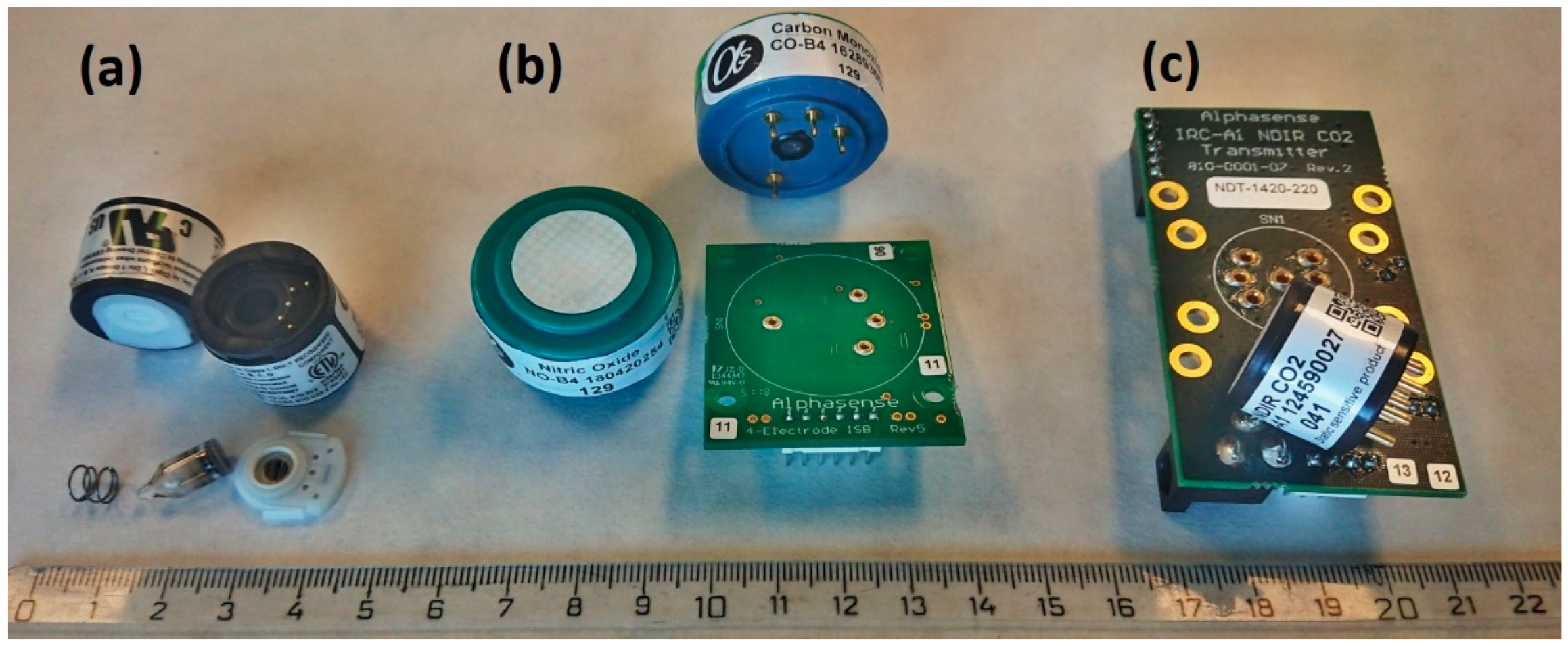
2.2. Sensor Theory and Selection
2.2.1. Photoionization Detector (PID) Sensors
2.2.2. Electrochemical Sensors: Alphasense B4 Series
2.2.3. Carbon dioxide sensor CO2-IRC-A1
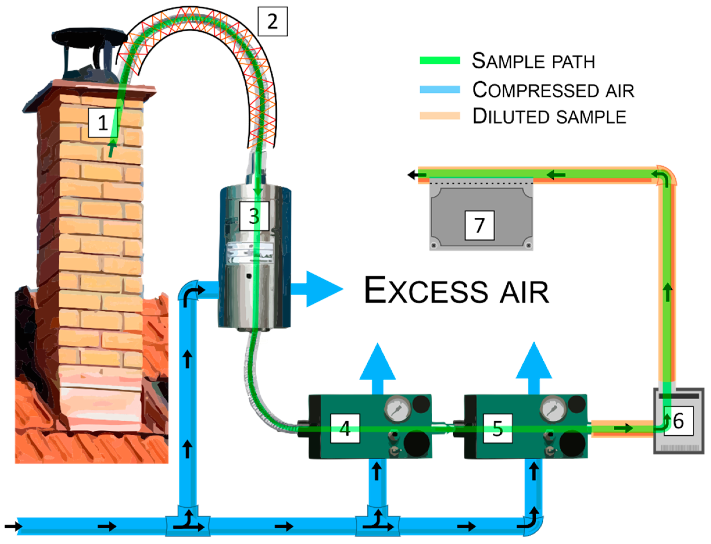
2.3. Sampling and Dilution Route
2.4. Reference Methods for Experimental Monitoring
2.5. Statistics
3. Results
3.1. Sample Transport and Dilution
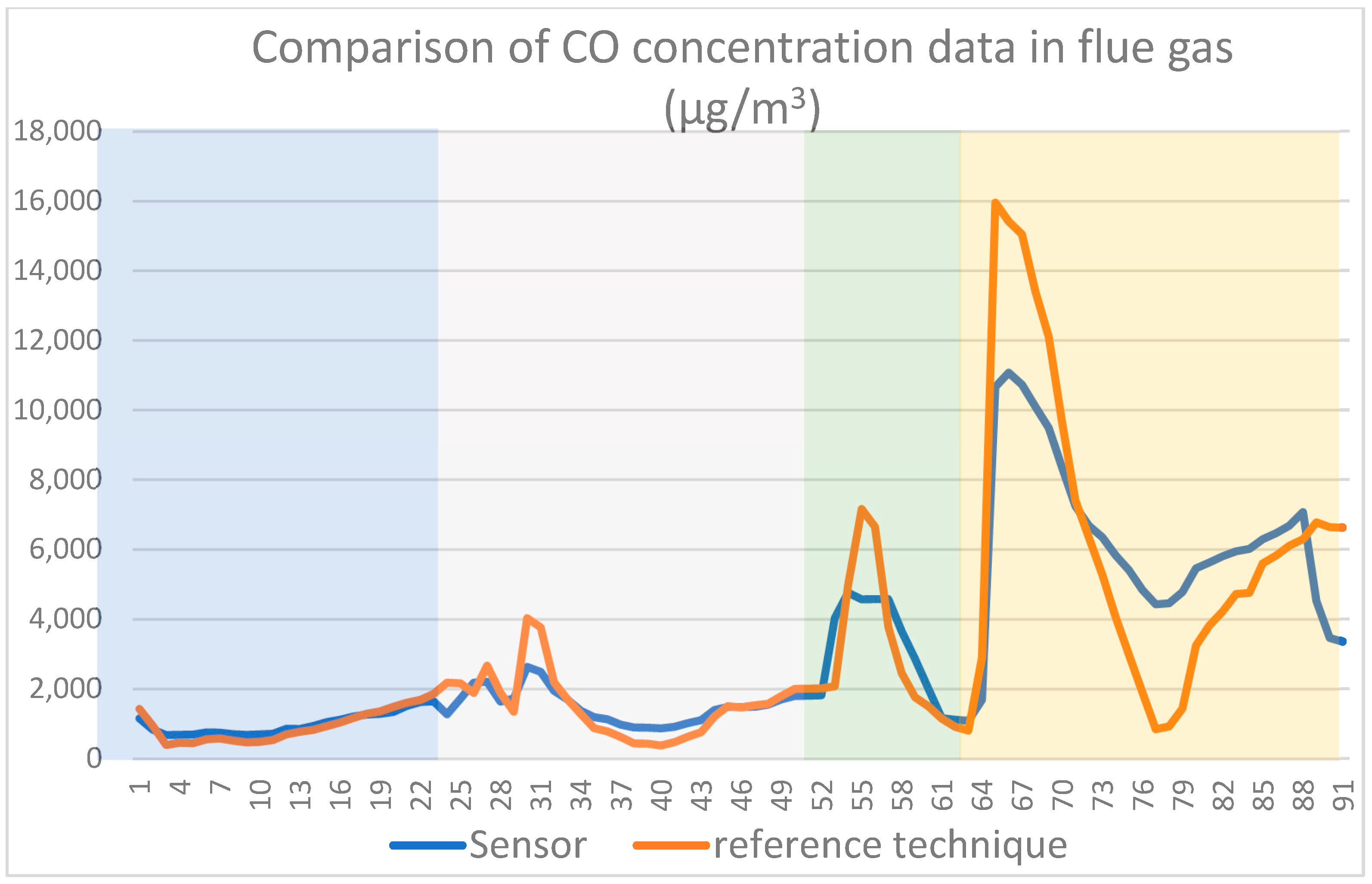
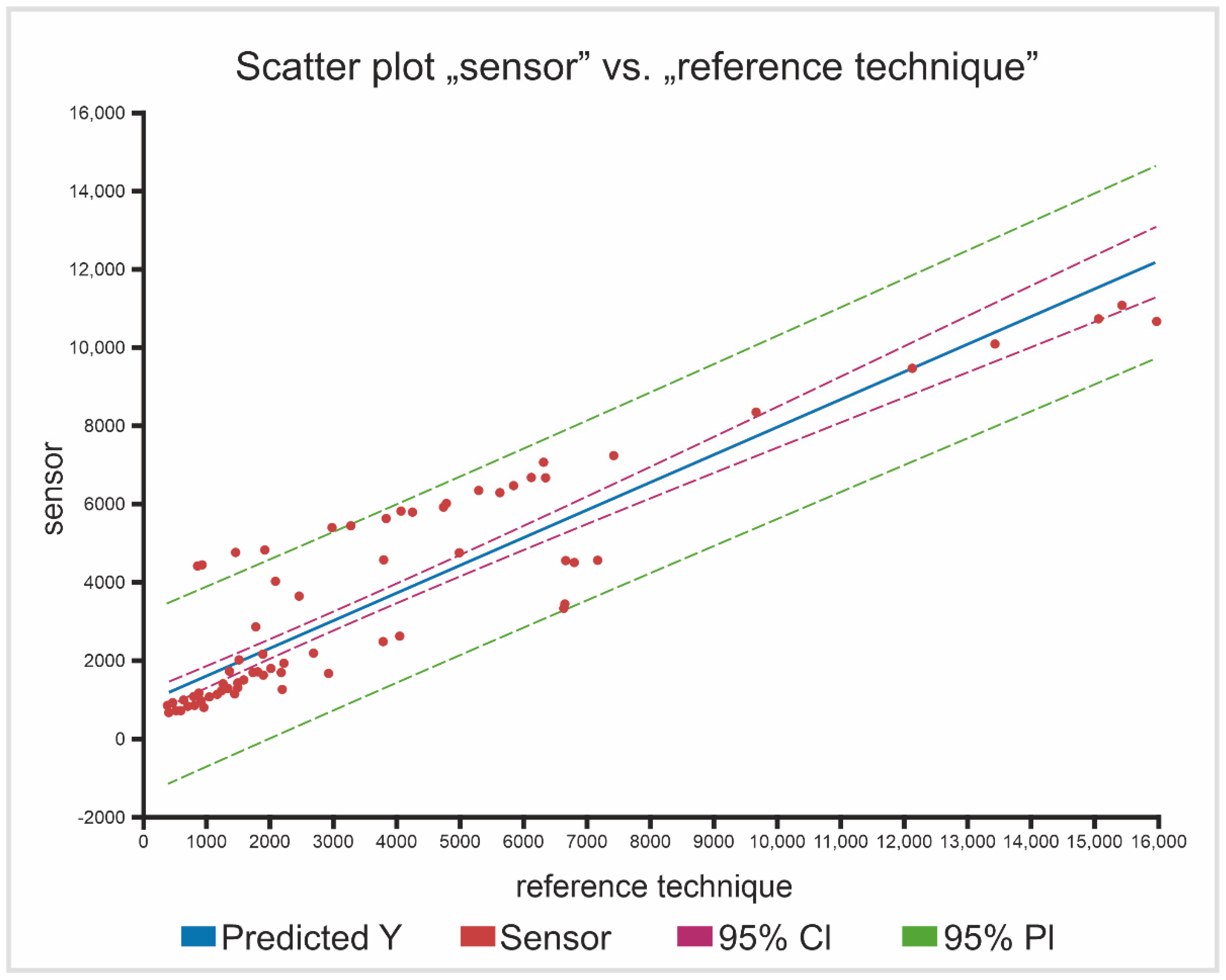
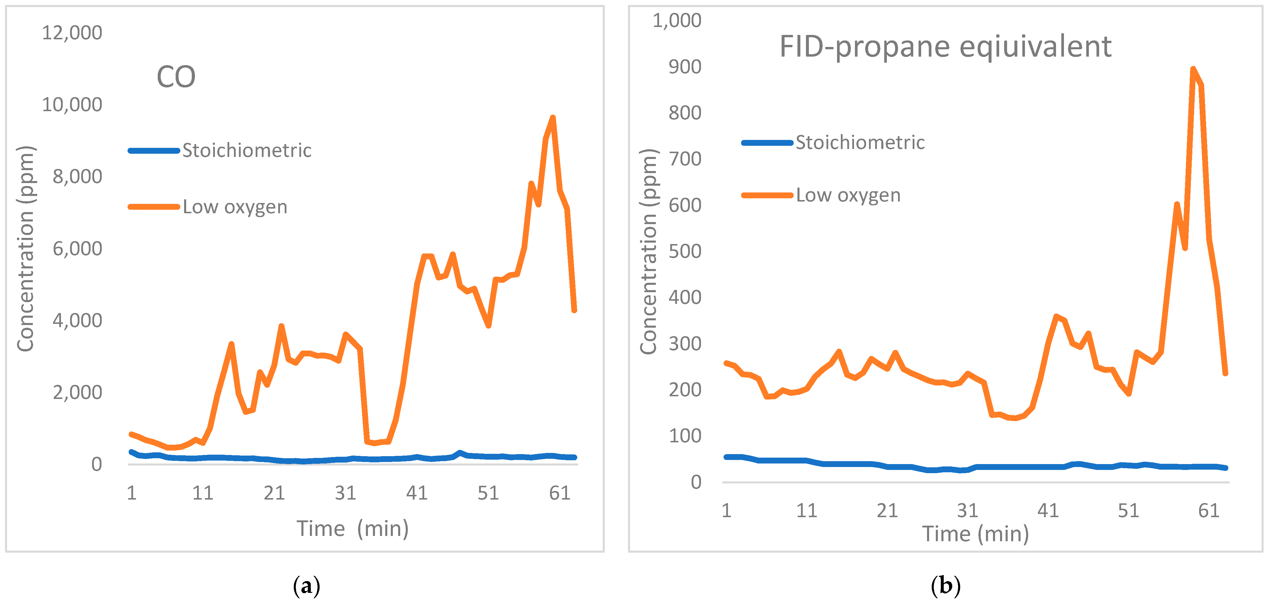
3.2. CO Sensors
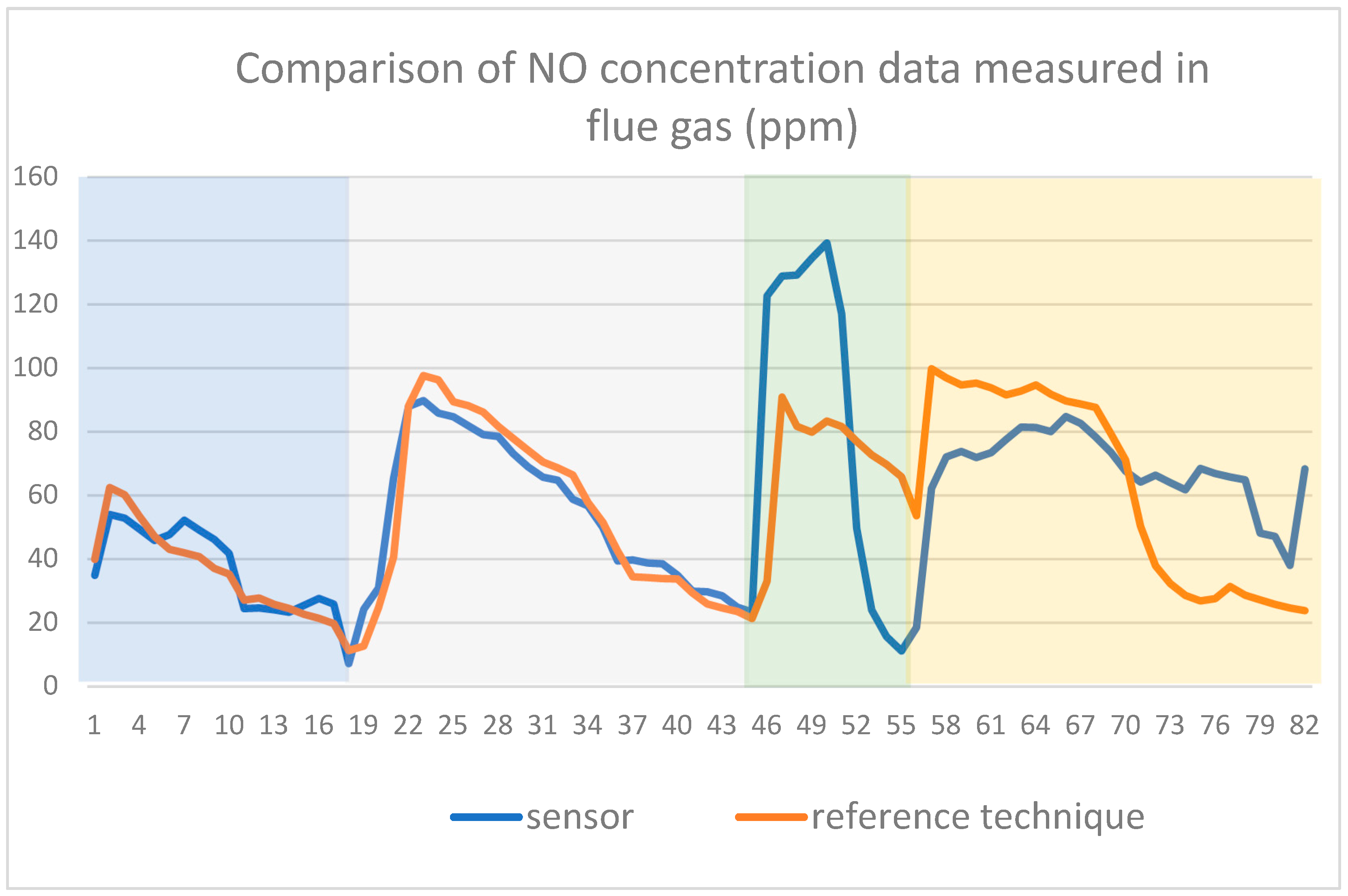
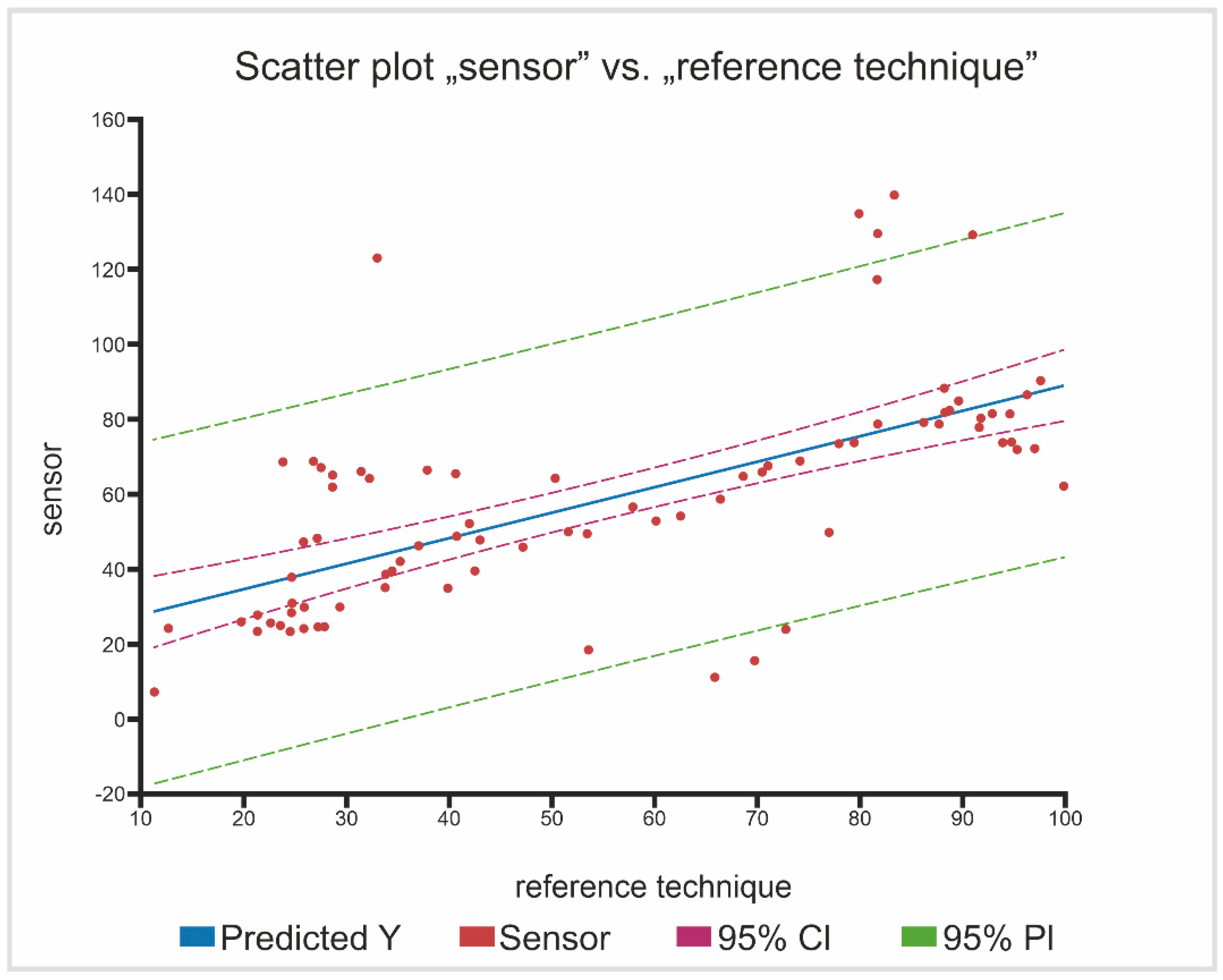
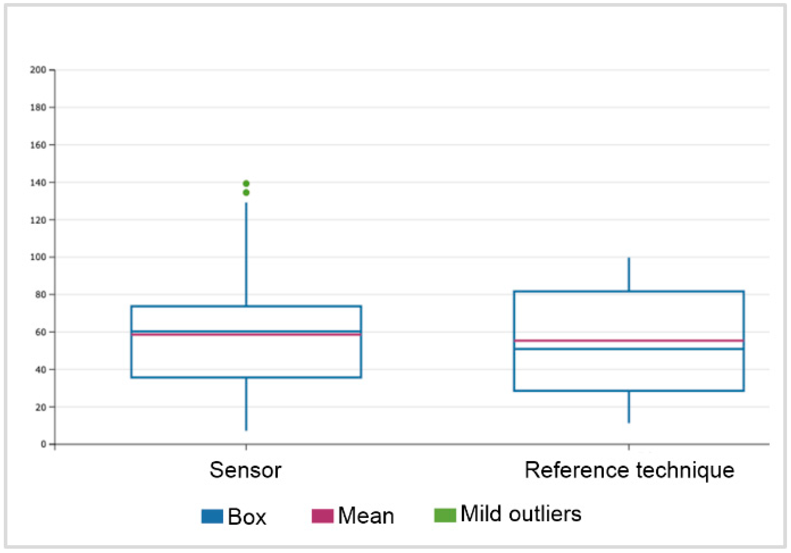
3.3. NO Sensors
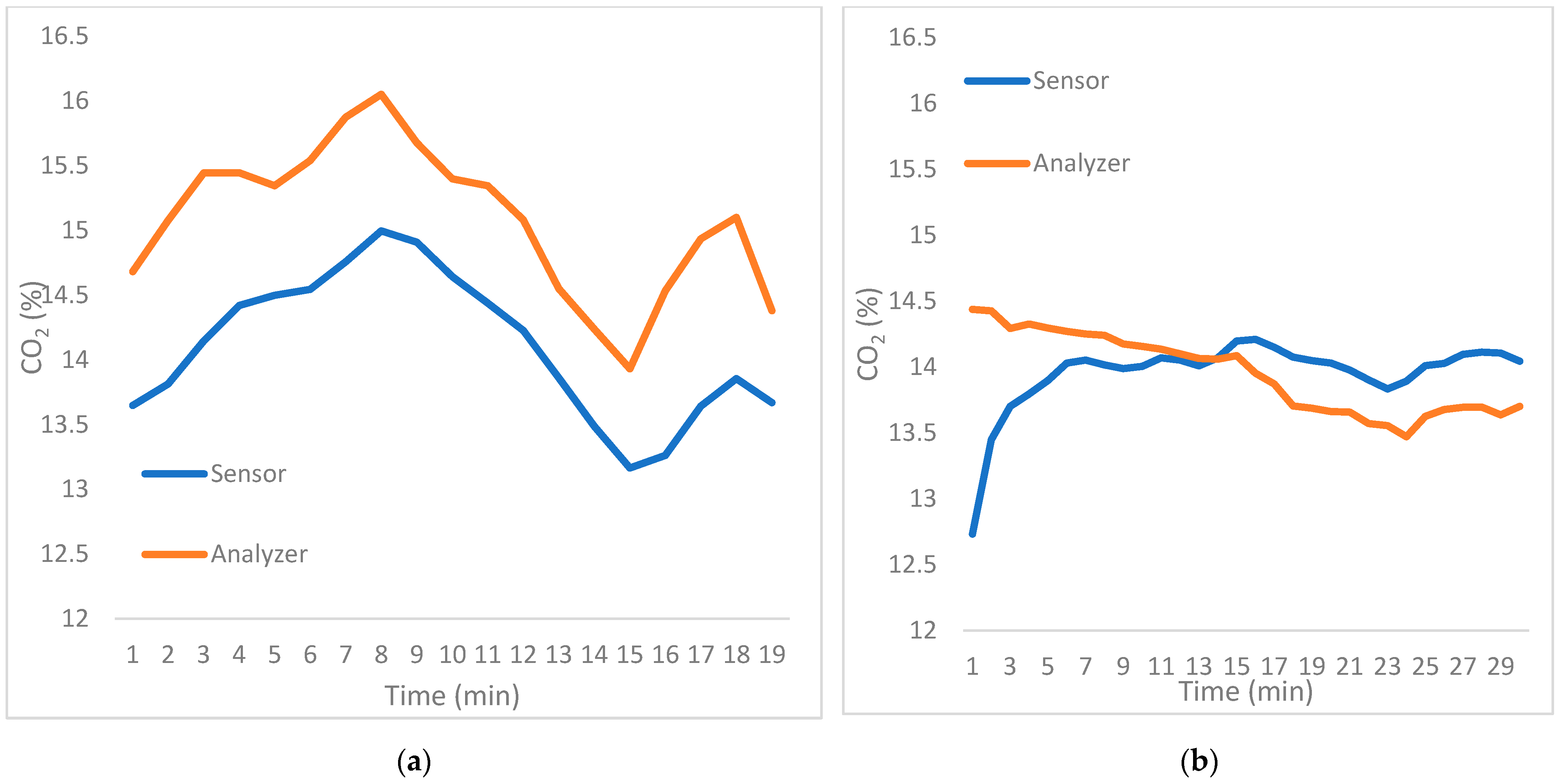
3.4. CO2 Sensors
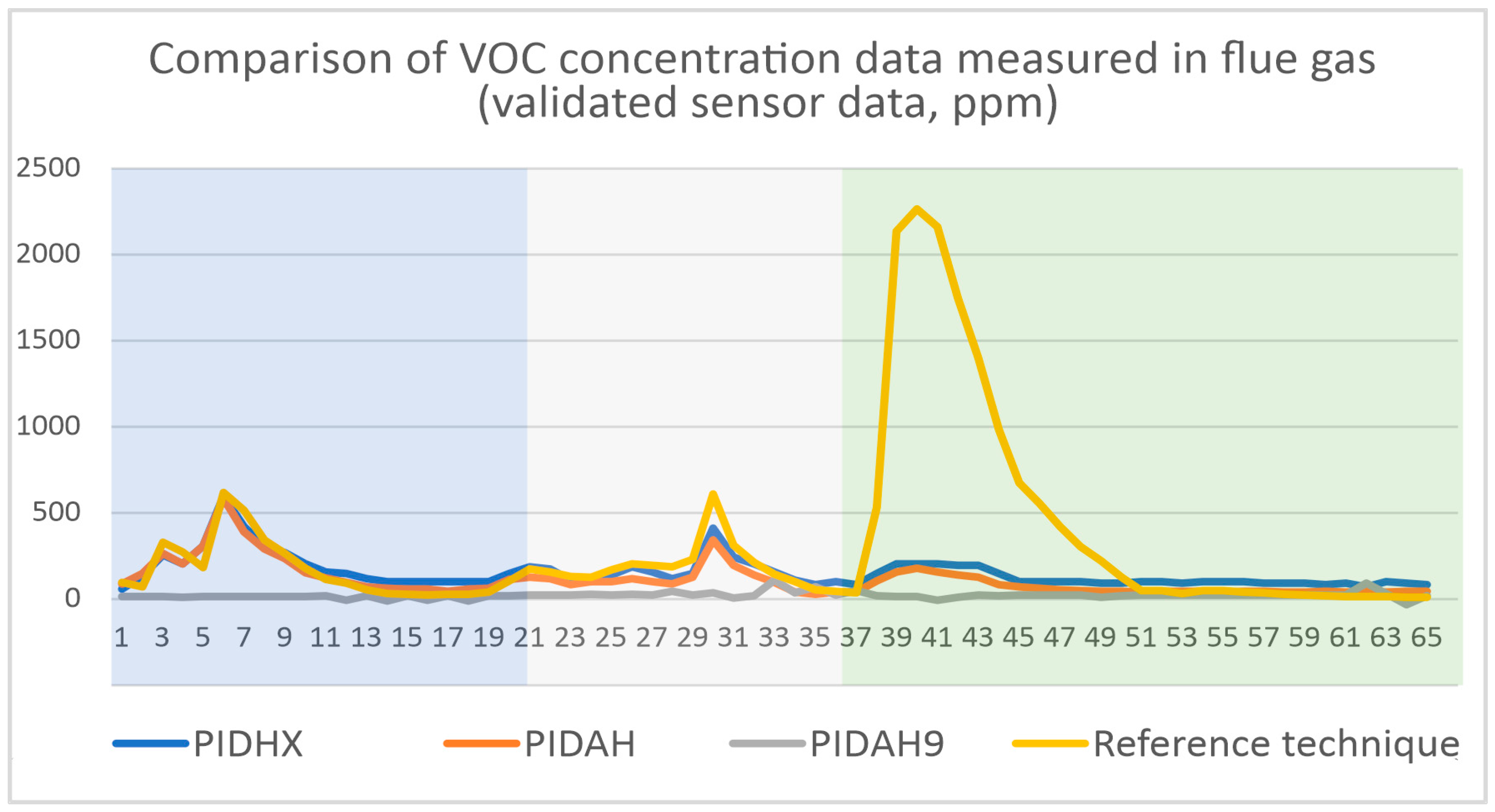
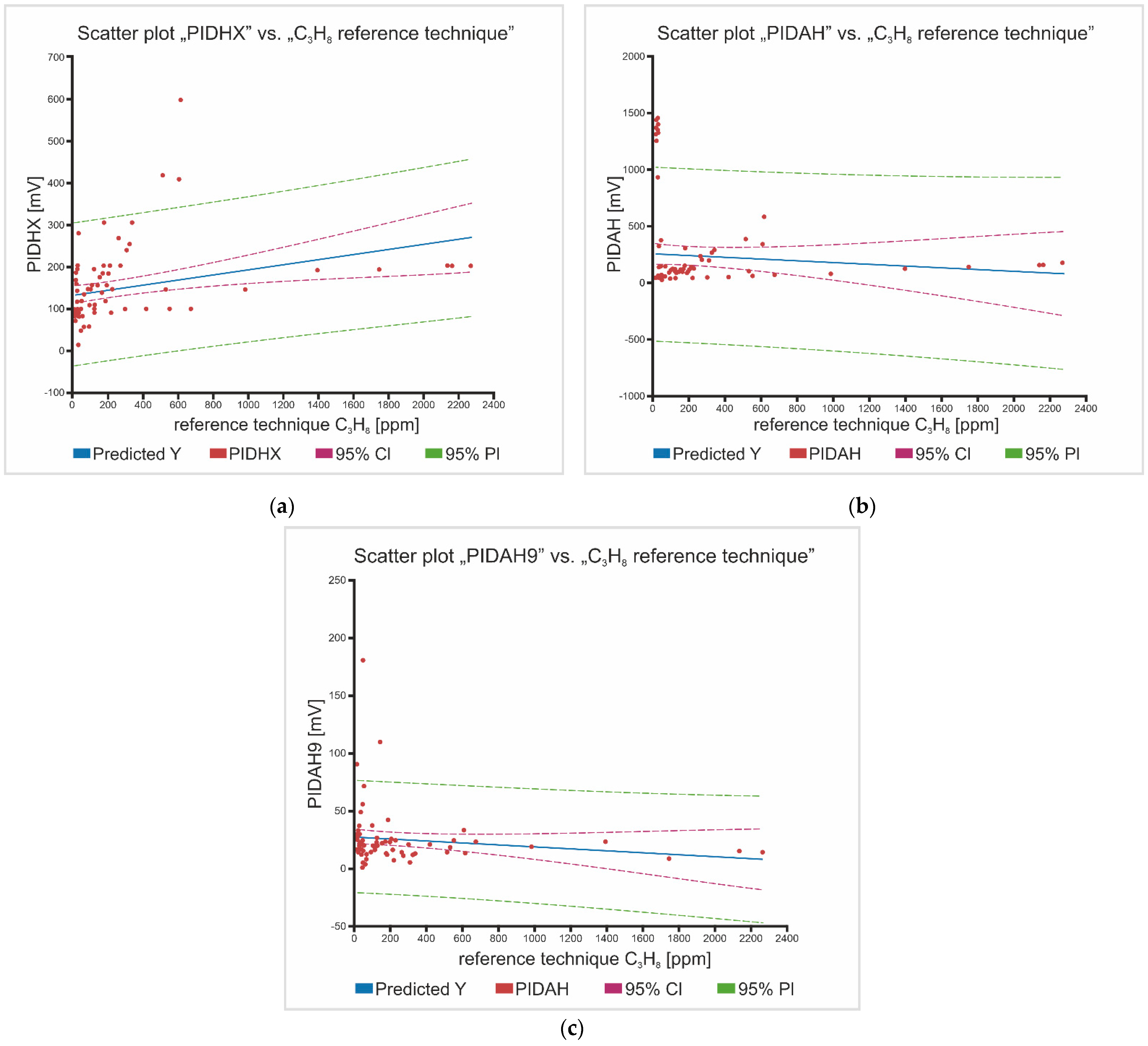
3.5. PID Sensors
4. Discussion
- Must not be used for continuous measurements (p11);
- Battery operation time circa 5 h (or 2.5 h, if gas cooler and IR module are on; p20);
- Measurements with pressure sensor must not be longer than 5 min (pp74/75).
5. Conclusions
Author Contributions
Funding
Data Availability Statement
Acknowledgments
Conflicts of Interest
References
- CHMI Air Quality Department—Annual Tabelar Overview. Available online: https://www.chmi.cz/files/portal/docs/uoco/isko/tab_roc/tab_roc_CZ.html (accessed on 24 May 2021).
- Krpec, K.; Horák, J.; Laciok, V.; Hopan, F.; Kubesa, P.; Lamberg, H.; Jokiniemi, J.; Tomšejová, Š. Impact of Boiler Type, Heat Output, and Combusted Fuel on Emission Factors for Gaseous and Particulate Pollutants. Energy Fuels 2016, 30, 8448–8456. [Google Scholar] [CrossRef]
- Křůmal, K.; Mikuška, P.; Horák, J.; Hopan, F.; Krpec, K. Comparison of Emissions of Gaseous and Particulate Pollutants from the Combustion of Biomass and Coal in Modern and Old-Type Boilers Used for Residential Heating in the Czech Republic, Central Europe. Chemosphere 2019, 229, 51–59. [Google Scholar] [CrossRef] [PubMed]
- Buček, P.; Maršolek, P.; Bílek, J. Low-Cost Sensors for Air Quality Monitoring—The Current State of the Technology and a Use Overview. Chem.-Didact.-Ecol.-Metrol. 2021, 26, 41–54. [Google Scholar] [CrossRef]
- Decree 415/2012 Sb.; Decree on the Permissible Level of Pollution and Its Determination and on the Implementation of Certain Other Provisions of the Air Protection Act. FAO/FAOLEX: Prague, Czech Republic, 2012.
- Commission Regulation (EU) 2015/1189 of 28 April 2015 Implementing Directive 2009/125/EC of the European Parliament and of the Council with Regard to Ecodesign Requirements for Solid Fuel Boilers (Text with EEA Relevance). 2015, Volume 193. Available online: http://data.europa.eu/eli/reg/2015/1189/oj/eng (accessed on 14 January 2022).
- Spinelle, L.; Gerboles, M.; Villani, M.G.; Aleixandre, M.; Bonavitacola, F. Field Calibration of a Cluster of Low-Cost Available Sensors for Air Quality Monitoring. Part A: Ozone and Nitrogen Dioxide. Sens. Actuators B Chem. 2015, 215, 249–257. [Google Scholar] [CrossRef]
- Spinelle, L.; Gerboles, M.; Villani, M.G.; Aleixandre, M.; Bonavitacola, F. Field Calibration of a Cluster of Low-Cost Commercially Available Sensors for Air Quality Monitoring. Part B: NO, CO and CO2. Sens. Actuators B Chem. 2017, 238, 706–715. [Google Scholar] [CrossRef]
- Karagulian, F.; Borowiak, A.; Barbiere, M.; Kotsev, A.; Van den Broecke, J.; Vonk, J.; Signorini, M.; Gerboles, M. Calibration of AirSensEUR Boxes during a Field Study in the Netherlands; European Commission: Ispra, Italy, 2020. [Google Scholar]
- De Vito, S.; Esposito, E.; Castell, N.; Schneider, P.; Bartonova, A. On the Robustness of Field Calibration for Smart Air Quality Monitors. Sens. Actuators B Chem. 2020, 310, 127869. [Google Scholar] [CrossRef]
- Tancev, G.; Pascale, C. The Relocation Problem of Field Calibrated Low-Cost Sensor Systems in Air Quality Monitoring: A Sampling Bias. Sensors 2020, 20, 6198. [Google Scholar] [CrossRef] [PubMed]
- Bílek, J.; Bílek, O.; Maršolek, P.; Buček, P. Ambient Air Quality Measurement with Low-Cost Optical and Electrochemical Sensors: An Evaluation of Continuous Year-Long Operation. Environments 2021, 8, 114. [Google Scholar] [CrossRef]
- Bílek, J.; Maršolek, P.; Bílek, O.; Buček, P. Field Test of Mini Photoionization Detector-Based Sensors—Monitoring of Volatile Organic Pollutants in Ambient Air. Environments 2022, 9, 49. [Google Scholar] [CrossRef]
- Alphasense Ltd. Technical Specifications: PID-A12. Available online: http://www.alphasense.com/WEB1213/wp-content/uploads/2019/08/PID-A12-1.pdf (accessed on 16 May 2020).
- Poole, C.F. Ionization-Based Detectors for Gas Chromatography. J. Chromatogr. A 2015, 1421, 137–153. [Google Scholar] [CrossRef] [PubMed]
- MSA Safety Data Sheet-0800-32. Available online: http://media.msanet.com/NA/USA/PortableInstruments/CombinationInstrumentsandCombustibleGasIndicators/SiriusMultigasDetector/0800-32.pdf (accessed on 30 November 2020).
- Coelho Rezende, G.; Le Calvé, S.; Brandner, J.J.; Newport, D. Micro Photoionization Detectors. Sens. Actuators B Chem. 2019, 287, 86–94. [Google Scholar] [CrossRef]
- Alphasense Ltd. Technical Specifications: PID-AH2. Available online: https://www.alphasense.com/wp-content/uploads/2019/08/PID-AH2.pdf (accessed on 21 February 2020).
- Alphasense Ltd. Application Note 301-04: Introduction to PhotoIonisation Detection. Available online: http://www.alphasense.com/WEB1213/wp-content/uploads/2013/07/AAN_301-04.pdf (accessed on 21 February 2020).
- Alphasense Ltd. Application Note 104: How Electrochemical Gas Sensors Work. Available online: https://www.alphasense.com/wp-content/uploads/2013/07/AAN_104.pdf (accessed on 21 February 2020).
- Mead, M.; Popoola, O.; Stewart, G.; Landshoff, P.; Calleja, M.; Hayes, M.; Baldovi, J.; McLeod, M.; Hodgson, T.; Dicks, J.; et al. The Use of Electrochemical Sensors for Monitoring Urban Air Quality in Low-Cost, High-Density Networks. Atmos. Environ. 2013, 70, 186–203. [Google Scholar] [CrossRef]
- Szulczyński, B.; Gębicki, J. Currently Commercially Available Chemical Sensors Employed for Detection of Volatile Organic Compounds in Outdoor and Indoor Air. Environments 2017, 4, 21. [Google Scholar] [CrossRef]
- Alphasense Ltd. Technical Specifications: NO-B4. Available online: https://www.alphasense.com/wp-content/uploads/2019/09/NO-B4.pdf (accessed on 21 February 2020).
- Alphasense Ltd. Technical Specifications: CO-B4. Available online: https://www.alphasense.com/wp-content/uploads/2019/09/CO-B4.pdf (accessed on 21 February 2020).
- Schobert, H. Chemistry of Fossil Fuels and Biofuels, 1st ed.; Cambridge University Press: Cambridge, UK, 2013; ISBN 978-0-521-11400-4. [Google Scholar]
- Kishnani, V.; Verma, G.; Pippara, R.K.; Yadav, A.; Chauhan, P.S.; Gupta, A. Highly Sensitive, Ambient Temperature CO Sensor Using Tin Oxide Based Composites. Sens. Actuators A Phys. 2021, 332, 113111. [Google Scholar] [CrossRef]
- Verma, G.; Gupta, A. Recent Development in Carbon Nanotubes Based Gas Sensors. J. Mater. NanoSci. 2022, 9, 3–12. [Google Scholar]
- Testo Ltd. Testo 350—Instruction Manual. Available online: https://www.testo.com/en-UK/testo-350/p/0632-3510#tab-downloads (accessed on 12 June 2022).
- Henderson, R.E. Questions, Myths and Misconceptions—About Using Photoionization Detectors. Available online: http://www.envirotech-online.com/article/health-and-safety/10/bw-technologies-by-honeywell/questions-myths-and-misconceptions-about-using-photoionization-detectors-robert-e-henderson/935 (accessed on 12 January 2022).
- Senum, G.I. Quenching or Enhancement of the Response of the Photoionization Detector. J. Chromatogr. A 1981, 205, 413–418. [Google Scholar] [CrossRef]
- van Harrevelt, R. First Ultraviolet Absorption Band of Methane: An Ab Initio Study. J. Chem. Phys. 2007, 126, 204313. [Google Scholar] [CrossRef] [PubMed]


| Sensor Marking | Filling Gas | Ionization Energy (eV) | Measurement Range (ppm Isobutylene) |
|---|---|---|---|
| PID-H9 | Xenon | 9.6 | 0–8000 |
| PID-HX | Krypton 1 | 10.0 | 0–100 |
| PID-AH | Krypton | 10.6 | 0–40 |
| Sensed moiety | NO | CO |
| Limit of detection | 20 ppb | 4 ppb |
| Measurement range | 0–20 ppm | 0–500 ppm |
| Sensitivity | 1 ppb | 25 ppb |
| Uncertainty | <30% | <30% |
| Interference | H2S, NO2, Cl2, SO2 | H2S, NO2, Cl2, SO2 |
| Target substance | CO2 |
| Measurement range | 0–20% |
| Humidity range | 0–95% |
| Zero resolution | 1 ppm |
| Full-scale resolution | 500 ppm |
| Dilutors | Output Concentration | Dilution Factor |
|---|---|---|
| 1: VKL 10E | 2.09% | 9.5 |
| 2: VKL 10E + VKL 10 | 0.25% | 81.2 |
| 3: VKL 10E + 2xVKL 10 | 0.026% | 774 |
| Statistical Parameter | CO Sensor | Reference Analyzer |
|---|---|---|
| Arithmetic mean | 3088.2 µg/m3 | 3089.0 µg/m3 |
| Minimum | 684.8 µg/m3 | 386.1 µg/m3 |
| Maximum | 11,074.9 µg/m3 | 15,595.6 µg/m3 |
| Median | 1707.1 µg/m3 | 1708.7 µg/m3 |
| Geometric mean | 2184.2 | 1905.6 µg/m3 |
| Pearson | 0.91 | |
| Statistical Parameter | NO Sensor | Reference Analyzer |
|---|---|---|
| Arithmetic mean | 58.6 ppm | 55.4 ppm |
| Minimum | 7.2 ppm | 11.3 ppm |
| Maximum | 139.3 ppm | 99.8 ppm |
| Median | 60.3 ppm | 50.9 ppm |
| Geometric mean | 50.93 ppm | 48.0 ppm |
| Pearson | 0.64 | |
| Measurement | Sensor (% v/v) | Reference Analyzer (% v/v) | R | Duration (min) |
|---|---|---|---|---|
| Flue gas undiluted (S*) | 13.99 | 13.93 | 0.32 | 30 |
| Flue gas diluted 10× (S*) | 0.36 | 13.16 | 0.76 | 22 |
| Flue gas undiluted (LO) | 14.07 | 14.68 | 0.88 | 26 |
| Flue gas diluted 10× (LO) | 0.34 | 12.05 | 0.47 | 120 |
| Benzene (%) | PIDHX (mV) | PIDAH (mV) | PIDAH9 (mV) |
|---|---|---|---|
| 0.000 | 40.00 | 47.00 | 36.00 |
| 6.440 E-04 | 44.50 | 58.70 | 35.80 |
| 9.390 E-04 | 103.80 | 252.70 | 37.10 |
| 0.016 | 923.50 | 2374.00 | 53.80 |
| 0.100 | 2398.00 | 2373.00 | 160.00 |
| 0.961 | 2397.00 | 2373.00 | 954.00 |
| PIDHX vs. | R2 |
|---|---|
| Benzene (B) | 0.85 |
| Benzene + Toluene (T) | 0.61 |
| B + T + Ethylbenzene (E) | 0.39 |
| B + T + E + Xylene (X) | 0.31 |
| B + T + E + X + Styrene (S) | 0.29 |
| Statistical Parameter | PIDHX (ppm) | PIDAH (ppm) | PIDAH9 (ppm) | Reference Analyzer (ppm) |
|---|---|---|---|---|
| Arithmetic mean | 149.3 | 236.1 | 25.9 | 245.2 |
| Median | 117.3 | 96.7 | 22.2 | 54.6 |
| Pearson | 0.32 | 0.09 | 0.16 | - |
Disclaimer/Publisher’s Note: The statements, opinions and data contained in all publications are solely those of the individual author(s) and contributor(s) and not of MDPI and/or the editor(s). MDPI and/or the editor(s) disclaim responsibility for any injury to people or property resulting from any ideas, methods, instructions or products referred to in the content. |
© 2023 by the authors. Licensee MDPI, Basel, Switzerland. This article is an open access article distributed under the terms and conditions of the Creative Commons Attribution (CC BY) license (https://creativecommons.org/licenses/by/4.0/).
Share and Cite
Buček, P.; Bílek, J.; Maršolek, P.; Bílek, O. Can Air Quality Gas Sensors Be Used for Emission Monitoring of Small-Scale Local Air Pollution Sources? Pilot Test Evaluation. Atmosphere 2023, 14, 248. https://doi.org/10.3390/atmos14020248
Buček P, Bílek J, Maršolek P, Bílek O. Can Air Quality Gas Sensors Be Used for Emission Monitoring of Small-Scale Local Air Pollution Sources? Pilot Test Evaluation. Atmosphere. 2023; 14(2):248. https://doi.org/10.3390/atmos14020248
Chicago/Turabian StyleBuček, Pavel, Jiří Bílek, Petr Maršolek, and Ondřej Bílek. 2023. "Can Air Quality Gas Sensors Be Used for Emission Monitoring of Small-Scale Local Air Pollution Sources? Pilot Test Evaluation" Atmosphere 14, no. 2: 248. https://doi.org/10.3390/atmos14020248
APA StyleBuček, P., Bílek, J., Maršolek, P., & Bílek, O. (2023). Can Air Quality Gas Sensors Be Used for Emission Monitoring of Small-Scale Local Air Pollution Sources? Pilot Test Evaluation. Atmosphere, 14(2), 248. https://doi.org/10.3390/atmos14020248