Article

Fractal Dimensions of Biomass Burning Aerosols from TEM Images Using the Box-Grid and Nested Squares Methods

1
Department of Physics, North Carolina Agricultural and Technical State University, Greensboro, NC 27411, USA
2
Department of Chemistry, North Carolina Agricultural and Technical State University, Greensboro, NC 27411, USA
3
Cooperatives Institute for Research in Environmental Sciences, University of Colorado, Boulder, CO 80309, USA
4
NOAA Chemical Sciences Laboratory, Boulder, CO 80305, USA
*
Author to whom correspondence should be addressed.
Atmosphere 2023, 14(2), 221; https://doi.org/10.3390/atmos14020221
Submission received: 22 December 2022 / Revised: 14 January 2023 / Accepted: 18 January 2023 / Published: 20 January 2023
(This article belongs to the Special Issue Chemical and Morphological Characterization of Atmospheric Aerosols)

Abstract

:
The fractal dimension is a key parameter in quantifying the morphology of aerosol aggregates, which is necessary to understand their radiative impact. Here we used Transmission Electron Microscopy (TEM) images to determine 2D fractal dimensions using the nested square and box-grid method and used two different empirical equations to obtain the 3D fractal dimensions. The values ranged from 1.70 ± 0.05 for pine to 1.82 ± 0.07 for Eucalyptus, with both methods giving nearly identical results using one of the empirical equations and the other overestimated the 3D values significantly when compared to other values in the literature. The values we obtained are comparable to the fractal dimensions of fresh aerosols in the literature and were dependent on fuel type and combustion condition. Although these methods accurately calculated the fractal dimension, they have shortcomings if the images are not of the highest quality. While there are many ways of determining the fractal dimension of linear features, we conclude that the application of every method requires careful consideration of a range of methodological concerns.

1. Introduction

Biomass burning (BB) is a major source of carbonaceous particulate matter (PM) in the global atmosphere [1,2,3,4]. The optical and chemical properties of PM emitted by biomass fuels are dependent on the fuel type, aging, and combustion conditions. Combustion conditions can range from a dominant flaming to dominant smoldering combustion [5,6,7,8]. Flaming combustion produces predominantly black carbon particles consisting of fractal chain aggregates that strongly absorb over the entire solar spectrum [9]. Smoldering combustion, on the other hand, produces mostly organic aerosols; part of which is called brown carbon (BrC), which predominantly absorbs at short visible and near-UV wavelengths [10,11,12,13]. The physical and optical characteristics of these BB aerosols are determined by a combination of their morphology, monomer size, and shape [14,15,16].
The effects of morphology on the optical properties of light absorbing aerosols, such as black carbon, have been widely studied [17,18,19]. However, by far the most widespread method for computing the optical properties of BB aerosols is to approximate aerosols as homogeneous spheres (i.e., Mie Theory) or with a core–shell morphology that assumes BB aerosols are uniformly coated by a concentric shell of weakly absorbent material [20]. However, the real morphology of BB aerosols is generally very complex and is dependent on the degree of aging, burning condition, fuel type, and relative humidity [21,22].
Combustion-generated aggregates such as soot from BB are usually composed of primary particles as self-duplicating units that form irregularly shaped clusters because of complex nucleation and aggregation processes [23]. These aggregates differ in their size, shape, radius of gyration, and particle density, and they exhibit complex geometry that can be characterized as mass fractals. The number of primary particles per aggregate, N, scales with the radius of gyration, Rg, as follows [24,25,26,27,28,29]:
N = k o ( R g a ) D f
and
N = k ( A a A p ) α
where Df is the three-dimensional fractal dimension, ko is the fractal pre-factor, a is the radius of the monomer, k is a pre-factor, Aa is the projected area of the aggregate, Ap is the projected area of the monomer, and α is the overlap parameter (the ratio of the monomer diameter to the distance between the centers of two touching monomers) [5,30,31,32,33,34,35,36]. However, calculating the overlap parameter, α, and the pre-factor, k, is difficult due to the level of image analysis required.
The fractal dimension is a decimal value that denotes the complexity of fractal, geometric shapes possessing self-similarity, such as the BB aerosols. The study of fractals occurs in a multitude of fields ranging from the study of root systems to image compression to the study of particulate matter in the atmosphere [37,38]. In this study we differentiate fractal dimension values by whether they were obtained by directly measuring the three-dimensional aerosol” by directly calculating the three-dimensional fractal dimensions using Eq. 1 or experimentally. The three-dimensional fractal dimension is the fundamental parameter to describe a fractal system and can be calculated based on the perimeter or the density. The two-dimensional (2D) density fractal dimension and the two-dimensional perimeter fractal dimension are two distinct dimensions that can be obtained by examining a two-dimensional image of an aerosol. The two-dimensional density fractal dimension describes the space-filling characteristics of the aggregate while the two-dimensional perimeter fractal dimension describes “the two-dimensional texture of the aggregate” [5,39]. Generally, the two-dimensional fractal dimension is used as an approximation for three-dimensional fractal dimension [5,39], but some use the two-dimensional perimeter fractal dimension instead [31].
The 3D fractal dimension is directly related to the geometry and structure of the aerosol and affects how the radiative properties change as the size of the aerosol changes [39,40]. Furthermore, aerosols such as soot mix with each other and change shape and fractal dimension in the atmosphere, resulting in changes in their optical properties [41]. To understand the effect of morphology and fractal dimensions on aerosol optical properties, it is necessary to characterize irregularly shaped objects on the basis of how their volumes vary relative to their size. This provides a statistical index to describe the morphology of the object: the fractal dimension [42].
Scanning electron microscopy (SEM) or Tunneling electron microscopy (TEM) is often used to provide a direct observation of the morphology, monomer size, and shape of the aerosol [34,39,41]. Analysis of TEM/SEM images involves the extraction of the three-dimensional (3D) fractal dimensions from the 2D projected images [27,43]. While several methods have been developed to obtain fractal dimensions from pixelated 2D images, the ensemble method (EM) is the most widely used and determines Df using Equation (1). Empirical relationships to determine 3D fractal dimensions from 2D results have also been developed [25,26,28,39,44].
In this work, we used two methods to calculate the 2D fractal dimension of biomass burning aerosols collected on filters from controlled laboratory experiments and imaged using TEM. These methods were the nested squares method (NSM) and the box-grid method (BGM). The methods were performed on several BB aerosols obtained by combusting African biomass fuels under flaming-dominated combustion conditions. Previous work has related the two-dimensional fractal dimension Dp to the mass fractal dimension Df (3-d) using the empirical relationship [31,44]:
D f = 1 + (   3 D p ) 3 2 ;   D f 2           D f = D p ; D f < 2
A second empirical relationship used was derived from a linear regression model providing a relationship between the 2D fractal dimension and the 3D fractal dimensions using [39]:
D f = 1.391 + 0.01 e 2.164 D p
Here, we examined the two-dimensional fractal dimensions calculated using the NSM and the BGM and the three-dimensional fractal dimensions obtained using Equations (3) and (4) and compared them with the experimental results in the literature for BB aerosols.

2. Materials and Methods

The filter samples were collected at the North Carolina Agricultural and Technical State University (NCAT) indoor burning facility, as described below [8,35,45]. The BB aerosol was generated by the combustion of Eucalyptus, Pine, and Olive wood fuels in a tube furnace. The furnace (Carbolite Gero, HST120300-120SN) holds an 85 mm OD, 80 mm ID, and 750 mm long quartz working tube with a heated region of 300 mm. Compressed house air passes through a zero-air generator (Aadco Instruments, 747-30) to provide zero air to the tube furnace through stainless steel tubing with the flowrate (10 standard liters per minute) controlled by a mass flow controller (MFC, Sierra Instruments). The fuel samples were placed in a quartz combustion boat (AdValue Technology, FQ-BT-03) and moved at the center of the furnace for the ignition. The temperature of the furnace can be adjusted from room to 1000 °C as desired. For this, work samples were burned at 750 °C and 800 °C. The burning conditions were determined from the modified combustion efficiency (MCE calculated using Equation (5) [46]:
M C E = Δ C O 2 Δ C O 2 + Δ C O
With ∆CO and ∆CO2 as the change in concentration of carbon monoxide and carbon dioxide, respectively. An MCE greater than 0.95 represents flaming-dominated combustion and an MCE less than 0.92 represents smoldering-dominated combustion, with a transition region between [47].
The smoke particles were then impacted onto a 3-mm copper tunneling TEM 400 mesh grids (TED PELLA, INC, 01844) with a pore diameter of 10 µm, using a small pump at a flow rate of 1 L/min. The samples for the TEM analysis had thicknesses of 100–200 nm. The filter samples were imaged using a TEM image (Carl Zeiss Libra 120 Plus) operating at a 120-kV accelerating voltage using lanthanum hexaboride as the electron source. The TEM had a high precision stage with a ±75° tilt and contained an Omega energy filter, which allowed the selection of distinct electron energies for specimen viewing. The resolution of the CCD camera used was 1376 × 1032 pixels with 14-bit dynamic range.
The analysis of both NSM and the BGM used the TEM images, ImageJ, and MATLAB software for analysis. MATLAB was used to import the data from ImageJ and create linear functions, as described in Section 2.1 and Section 2.2, to determine the 2D fractal dimension of the aggregate.
Before the TEM images were examined using the NSM and BGM, the images were altered to allow the pixels, which denote the presence of an aerosol aggregate, to be the only thing measured by ImageJ. The bottom of the image which contains information about the TEM image was cropped out. Next, the image was thresholded and converted into binary, converting the image to black and white. The scale was set to one unit per pixel and the area, min, and max gray value, and limit to threshold boxes under “set measurements” were checked. Finally, redirect needed to be set to none and the decimals to three significant figures [32]. These prerequisites were carried out using the macro shown in Supplement Material S1. Figure 1 shows what the TEM image of the aerosol should look like before and after this process.

2.1. Nested Square Method (NSM)

The NSM is used to calculate the two-dimensional density fractal dimension. This involves drawing squares or circles of increasing size that are measured from the center of mass of the aggregate [48]. For each boundary the number of pixels occupied by the particle is counted. The natural logarithm of the number of “on” pixels (pixels containing the aggregate after the image has been altered) in each box is plotted against the natural logarithm of the length of the edge of each square [42]. This method can result in a linear function that does not accurately agree with the data points due to outliers measured towards the end of the iterations. In this case, it is necessary to exclude the data points towards the end that begin to level off to calculate a more accurate fractal dimension based on the linear portion [42]. This method is illustrated in Figure 2.

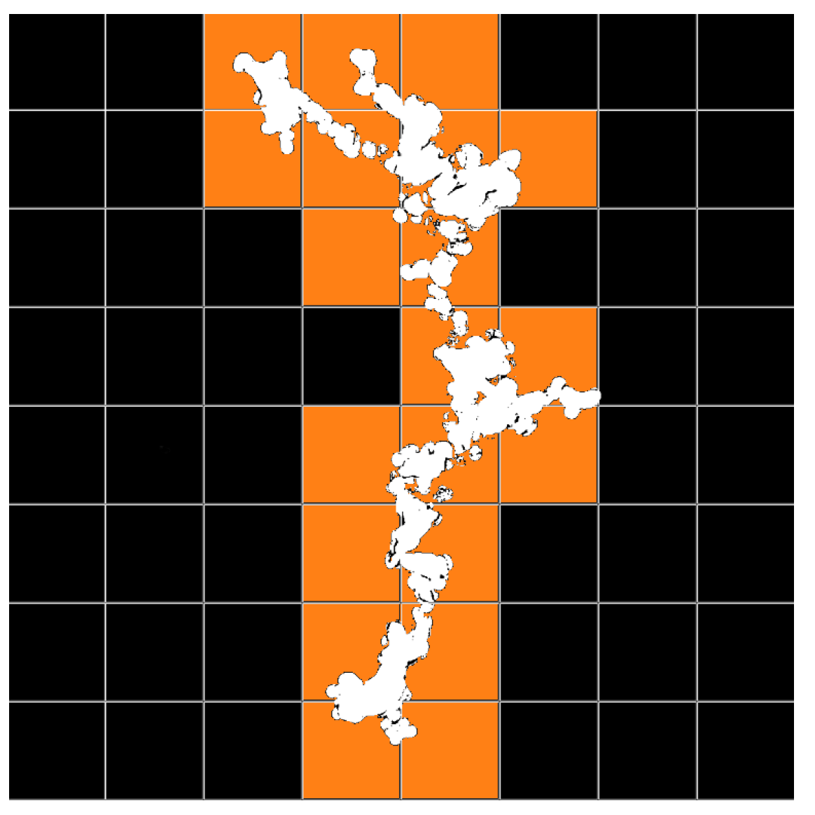
2.2. Box-Grid Method (BGM)
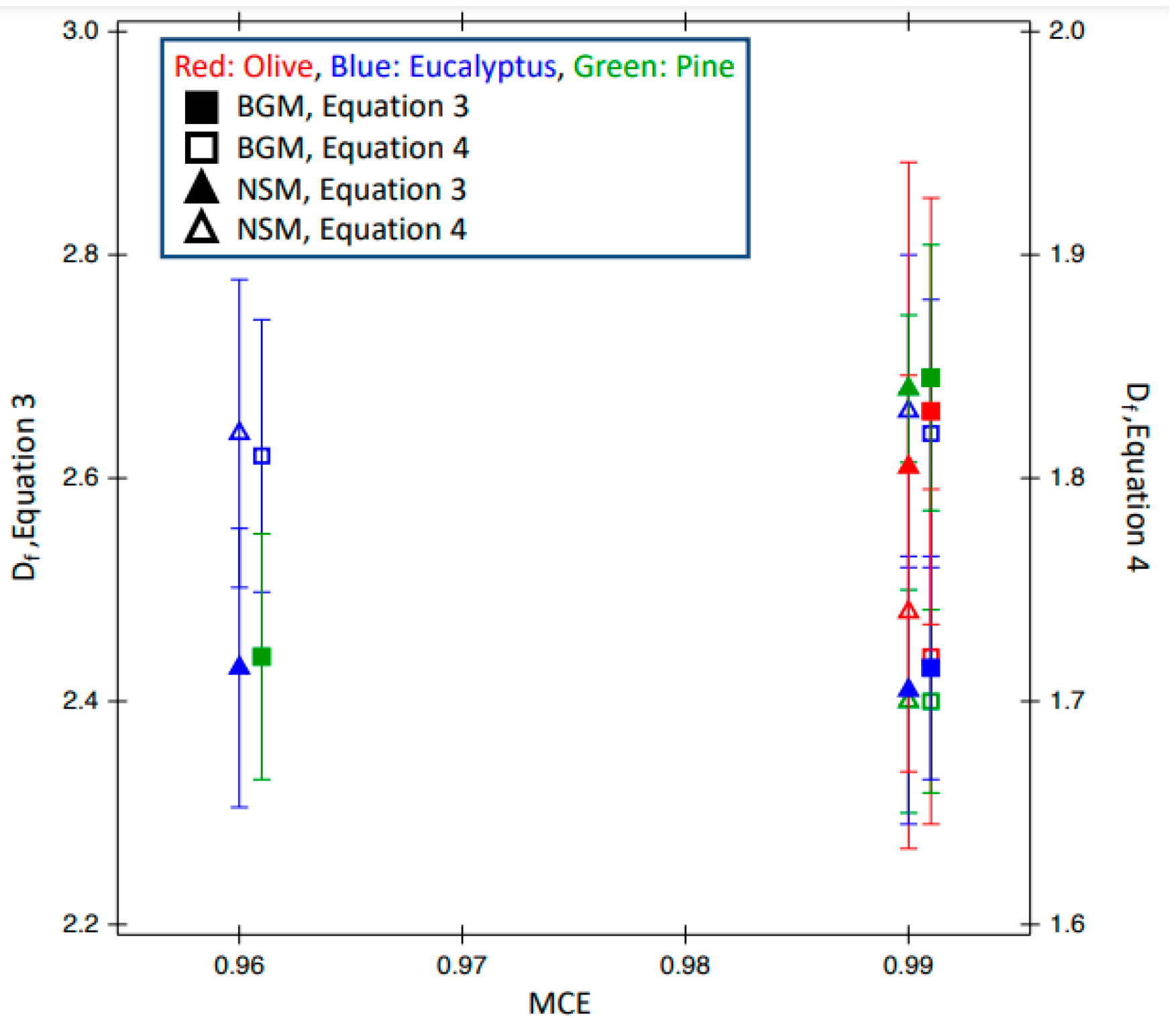
The BGM, also called the perimeter grid method [48] or box counting method [49], is used to calculate the density or perimeter fractal dimension. It works by generating a grid of squares over the image and counting the number of squares that contain the aggregate (or only the perimeter of the aggregate for the perimeter fractal dimension). This is then repeated several times while decreasing the length of the edge of the squares that make up the grid. The natural logarithm of the number of boxes containing the aggregate (or aggregate perimeter) is plotted against the log of the box’s edge length to calculate the fractal dimension [31,34,50,51,52]. This method is illustrated below in Figure 3. This method is also used to analyze irregular coastlines as depicted in Husain’s study [53].

3. Results

Using BGM and NSM, we analyzed 65 TEM images of biomass burning aerosols from flaming-dominated (MCE > 0.95) combustion of Eucalyptus, Olive, and Pine wood samples. Sample TEM images for all three fuels are shown in Figure 4.
The values of 2D fractal dimensions were in the range 1.47 to 1.94 using the BGM and in the range 1.49 to 1.82 using the NSM and they can be found in the Supplemental document S2. The results were dependent on fuel type and on combustion conditions. The empirical Equations (3) and (4) were used to calculate the 3D fractal dimensions. Average 2D and 3D fractal dimensions and standard deviations are in Table 1 and Figure 5 shows the plot of MCE vs. 3D fractal dimensions derived from each method and the equation for all fuels. The dependence on fuel type and MCE is clearly shown in the figure.

4. Discussions

4.1. Comparing Fractal Dimensions with the Literature Values

Our work studied the PM freshly emitted from the combustion of individual biomass fuels from Africa and the US under controlled laboratory conditions and found 2D fractal dimensions, Dp from 1.47 to 1.94, which were within the range of values reported in the literature [5,31,32,42,54]. Previous measurements involved both laboratory and field measurements of biomass burning aerosols from the combustion of mixed wildland fuels from North and South America and roadside urban samples from diesel emissions for both fresh and aged samples [55,56]. The range of Df determined computationally and experimentally for soot, silica, and black carbon lay in the range 1.6–1.9 [30], which was confirmed experimentally using image analysis and light scattering predictions [25,57]. Analysis of field studies by McDonald and Biswas [54] using the NSM yielded Dp between 1.39 and 1.89, while their BGM analysis yielded Dp between 1.66 and 1.83. In some studies, changes in morphology with fuel type have been observed, similar to ours [58]. Using the same methodology Katrinak and Rez [42] found Dp values ranging between 1.35 and 1.89 for urban aerosols. The calculation by Dye et al. for urban roadside emissions was Df = 1.56 and 1.57 [59]. Using NSM, Samson found Dp values from 1.75 to 1.95 [60] for Acetylene soot. For diesel soot aggregates, Wentzel [56] found Dp values that were generally lower and more fractal, ranging between 1.44 and 1.55.
Chakrabarty [5] conducted a laboratory measurement of fractal dimensions of emissions from combustions of several biomass fuels such as sagebrush, wood, ponderosa wood, pine needles, etc. They found that Df was in the range of 1.67–1.83 and Dp was between 1.68 and1.74, which is similar to our results. In the field measurement studies of images of both ambient and denuded aerosols, China et al. [32] calculated the Df using Equation (1) and found 1.85 ± 0.05 for ambient and 1.53 ± 0.07 for denuded samples. Clearly, Df reflects the history of fractals and is controlled by combustion conditions and aging processes. In a study at urban, mountaintop, and background sites in China, the Df for fresh particles remained at a consistent value of 1.82 at all sites [41]. Most current studies put Df = 1.8 to simulate the structures of soot particles for optical properties calculations [35,61,62,63], but this value does not represent aged particles. A new method named soot parameters (SP) that uses Equation (1) with the scaling law and image recognition technology to automatically determine Df was used to show differences in Df values for soot particles from cars (1.66 ± 0.17), BB aerosols (1.75 ± 0.18), and coal burning aerosols (1.76 ± 0.18) [33,64].
In our recent study [47], we examined the physical and morphological properties of aerosols emitted from six different types of hardwood fuels native to sub-Saharan Africa under controlled laboratory burning conditions. The mass mobility exponent of Dfm which is the 3D fractal dimension for fresh aerosol emitted during flaming-dominated emissions was 2.26 ± 0.05 and commensurate with previously studied externally mixed BC and diesel exhaust particles. The 3D fractal dimensions for biomass burning aerosols were in the range 1.67–1.83 determined using Equation (1) from TEM images in one study or 1.85 in another [41]. These values are within the range of our values obtained by using the empirical Equation (4) to convert the 2D fractal dimensions calculated from NSM and BGM. However, the values were much larger when using empirical Equation (3) to the point of being unreasonable. Since these values were also larger than what we experimentally determined for the flaming-dominated combustion of similar fuels and other values in the literature, Equation (3) is not appropriate for flaming-dominated BB aerosols.

4.2. BGM Considerations

Chakrabarty et al. [48] reported on the validity, accuracy, and reliability of the most used analysis techniques for the determination of Df of both individual and ensemble aggregates. They compared both the NSM and BGM methods with the ensemble method (EM) calculation of fractal dimension based on Equation (1) and determined that EM was the only method that could be used to reliably determine Df from 2D images. They hypothesized that the errors in the value of Df by NSM and BGM were due to the “non-self-similar” property of aerosol aggregates and their 2D images. The repeating unit of a fractal object should appear similar under any magnification, but this assumption of “self-similarity” breaks as the length scale approaches the monomer size in most cases.
Another problem with the fractal dimensions estimated by BGM is due to the errors arising from arbitrary grid placement, which we call the grid placement error. It comes from miscalculating the minimum number of boxes of a certain size necessary to cover the object at a given scale. A modified box-counting-based method has been proposed to improve the fractal dimension estimate accuracy [65]. However, using the box-grid method to present the fractal dimension of a fractal object is widely accepted and acknowledged due to its close equivalence on small scale.
Box counting also requires many data points to produce a correct fractal dimension. Dubuc et al. [66] reported instabilities in the method when the number of data points used was small. They also found that the method was sensitive to the digitization process, the resulting quantization error, and the threshold used to determine the presence or absence of a particle in a given pixel. Quantization errors arise from the use of pixilated images that are produced from the digitization process and can affect the minimum number of boxes [67]. This sensitivity may apply to other methods and should be investigated.
Box counting can also suffer from a “remainder” problem. If the boxes cannot cover the particles evenly then some cells will be missed if the box sizes increase geometrically. Because of this potential problem, some authors have suggested first mapping the raw data onto a square unit [68].
Loading an image of a fractal and calculating its box-counting dimension is also used for its simplicity, which may sacrifice accuracy and many details due to the distortion occurred in deriving the fractal expression from a pixel image [49].
On the practical side, the box-grid method is highly sensitive to noise. This is because the box-grid method looks over every single pixel in the image. When aerosols and substrate structures overlap, BGM will give a fractal dimension value much lower or higher than the actual fractal dimension due to the loss of aerosol in the image or the inclusion of extra substrate in the image, respectively. In some cases, it is impossible to take TEM images of the aerosols without the substrate appearing in the image, meaning the only other course of action would be to edit out the substrate by hand. This can prove to be anything from difficult to impossible without losing the integrity and accuracy of the experiment.

4.3. NSM Considerations

The main problem with the NSM is that it requires that the user find the center of mass of the aerosol aggregate as the center for the nested squares. For many images, this point is obvious, but issues can still arise. First, a slight change in the center of the nested squares can result in an entirely different fractal dimension. For example, the same image produced two fractal dimension values that differed by 0.6 when the centers of the nested square were only 6 pixels apart. Second, the center of mass of the aerosol may not contain any amount of aerosol depending on the aerosol geometry, which is necessary for this method. For such cases, that image must be discarded or a point near the center of mass must be chosen. This severely hinders this method’s ease of use and ability to be used. Depending on the image, it may be necessary to change the starting size or increment size of the squares. This can occur for any number of reasons such as differences in aerosol size relative to the whole image, differences in geometry, or the presence of nearby particles producing interference. This can prove to be a great a hindrance when given a varied set of images.
To properly use the NSM, it is imperative to view the graph of the log of the pixel count versus the log of the box length and not only rely on the result of a linear fit. The presence of points far away from the fit line is indicative of an incorrect center of mass. Figure 6 illustrates a graph that indicates that the method was carried out correctly and the proper center of mass was selected.
When the line of best fit is lined up with the data points, the fractal dimension produced is acceptable. However, sometimes the mass of the aggregates is distributed unevenly around the center, causing an abrupt change in the slope. Therefore, the points on the plot corresponding to the largest nested squares may need to be excluded. They tend to level out which skews the line of best fit and by extension the fractal dimension as shown in Figure 6 [42], so the only the linear portion must be fit. Overall, the method of nested squares requires reducing the number of data point for the purposes of curve fitting to avoid the truncation effect.
In addition, the process of depositing aerosols on filters may lead to aggregates ending up in contact at multiple contact points on the filter surface and depending on the resting area the 2D projection area and length can be overestimated [69]. Because of this problem it is shown that NSM underestimates the resulting Df [70].

5. Conclusions

In this work, we used TEM images of BB aerosols to determine the 2D fractal dimensions using the BGM and NSM. The values ranged from 1.70 ± 0.05 for pine to 1.82 ± 0.07 for Eucalyptus with both methods giving nearly identical results using the empirical equation proposed by Lee (Equation (4)). Based on the results and comparison with reported values of fractal dimensions for BB aerosols, our results provided reasonable values. We can conclude that these are viable methods for future research in investigating the fractal dimensions of aerosols provided TEM images of the aerosols are available. This guarantees the NSM and BGM as technologically easy and non-labor-intensive methods to calculate the fractal dimensions of BB aerosols for future research. In converting the 2D fractal dimensions to 3D dimensions we found that the empirical Equation (4) provided reasonable values while the empirical Equation (3) overestimated the values and was unreasonable when compared to the literature values explored in this work. However, both methods behaved poorly when analyzing low quality images. In addition, they both have potential sources of error unique to them. The quantization error and substrate issue are potential concerns with regards to BGM and the graphing issue and the issue of choosing the correct center are unique to NSM. The main conclusion to be reached is that while there are many ways of determining the fractal dimension of linear features, the application of every method requires careful consideration of a range of methodological concerns. Without adequate consideration of the potential problems, the results from any analysis may not truly reflect the fractal nature of the feature.

Supplementary Materials

The following supporting information can be downloaded at: www.mdpi.com/article/10.3390/atmos14020221/s1, S1. Images and calculated values of Df; S2. Programs used.

Author Contributions

Conceptualization, R.P.P. and S.B.; Software, T.H.; Formal analysis, T.H.; Writing—original draft, T.H.; Writing—review & editing, M.N.F., R.P.P. and S.B.; Project administration, S.B.; Funding acquisition, S.B. All authors have read and agreed to the published version of the manuscript.

Funding

This research was funded The National Science Foundation (NSF), grant number AGS1831013.

Institutional Review Board Statement

Not applicable.

Informed Consent Statement

Not applicable.

Acknowledgments

This work was performed in whole/part at the Joint School of Nanoscience and Nanoengineering, a member of the National Nanotechnology Coordinated Infrastructure (NNCI), which is supported by the National Science Foundation (Grant ECCS-2025462). We also acknowledge the contributions of Megan Mouton in helping with the plots.

Conflicts of Interest

The authors declare no conflict of interest.

References

  1. Bond, T.C.; Doherty, S.J.; Fahey, D.W.; Forster, P.M.; Berntsen, T.; DeAngelo, B.J.; Flanner, M.G.; Ghan, S.; Kärcher, B.; Koch, D.; et al. Bounding the role of black carbon in the climate system: A scientific assessment. J. Geophys. Res. Atmos. 2013, 118, 5380–5552. [Google Scholar]
  2. Bond, T.C. Aerosol properties at a midlatitude northern hemisphere continental site. J. Geophys. Res. Atmos. 2001, 106, 3019–3032. [Google Scholar]
  3. Andreae, M.O. Emission of trace gases and aerosols from biomass burning—An updated assessment. Atmos. Chem. Phys. 2019, 19, 8523–8546. [Google Scholar] [CrossRef] [Green Version]
  4. Jiang, H.; Frie, A.L.; Lavi, A.; Chen, J.Y.; Zhang, H.; Bahreini, R.; Lin, Y.H. Brown Carbon Formation from Nighttime Chemistry of Unsaturated Heterocyclic Volatile Organic Compounds. Environ. Sci. Technol. Lett. 2019, 6, 184–190. [Google Scholar] [CrossRef]
  5. Chakrabarty, R.K.; Moosmüller, H.; Garro, M.A.; Arnott, W.P.; Walker, J.; Susott, R.A.; Babbitt, R.E.; Wold, C.E.; Lincoln, E.N.; Hao, W.M. Emissions from the laboratory combustion of wildland fuels: Particle morphology and size. J. Geophys. Res. Atmos. 2006, 111, 6659. [Google Scholar] [CrossRef] [Green Version]
  6. Reid, J.S.; Eck, T.F.; Christopher, S.A.; Koppmann, R.; Dubovik, O.; Eleuterio, D.P.; Holben, B.N.; Reid, E.A.; Zhang, J. A review of biomass burning emissions part III: Intensive optical properties of biomass burning particles. Atmos. Chem. Phys. 2005, 5, 827–849. [Google Scholar] [CrossRef] [Green Version]
  7. Martinsson, J.; Eriksson, A.C.; Nielsen, I.E.; Malmborg, V.B.; Ahlberg, E.; Andersen, C.; Lindgren, R.; Nystrom, R.; Nordin, E.Z.; Brune, W.H.; et al. Impacts of Combustion Conditions and Photochemical Processing on the Light Absorption of Biomass Combustion Aerosol. Environ. Sci. Technol. 2015, 49, 14663–14671. [Google Scholar] [CrossRef] [PubMed] [Green Version]
  8. Smith, D.M.; Fiddler, M.N.; Pokhrel, R.P.; Bililign, S. Laboratory studies of fresh and aged biomass burning aerosols emitted from east African biomass fuels—Part 1—Optical properties. Atmos. Chem. Phys. Discuss. 2020, 2020, 1–30. [Google Scholar] [CrossRef]
  9. Bond, T.C.; Bergstrom, R.W. Light Absorption by Carbonaceous Particles: An Investigative Review. Aerosol Sci. Technol. 2006, 40, 27–67. [Google Scholar] [CrossRef]
  10. Chen, Y.; Bond, T.C. Light absorption by organic carbon from wood combustion. Atmos. Chem. Phys. 2010, 10, 1773–1787. [Google Scholar] [CrossRef] [Green Version]
  11. Lack, D.A.; Langridge, J.M.; Bahreini, R.; Cappa, C.D.; Middlebrook, A.M.; Schwarz, J.P. Brown carbon and internal mixing in biomass burning particles. Proc. Natl. Acad. Sci. USA 2012, 109, 14802–14807. [Google Scholar] [CrossRef] [PubMed] [Green Version]
  12. Saleh, R.; Robinson, E.S.; Tkacik, D.S.; Ahern, A.T.; Liu, S.; Aiken, A.C.; Sullivan, R.C.; Presto, A.A.; Dubey, M.K.; Yokelson, R.J.; et al. Brownness of organics in aerosols from biomass burning linked to their black carbon content. Nat. Geosci. 2014, 7, 647–650. [Google Scholar] [CrossRef]
  13. Taylor, J.W.; Wu, H.; Szpek, K.; Bower, K.; Crawford, I.; Flynn, M.J.; Williams, P.I.; Dorsey, J.; Langridge, J.M.; Cotterell, M.; et al. Absorption closure in highly aged biomass burning smoke. Atmos. Chem. Phys. 2020, 20, 11201–11221. [Google Scholar] [CrossRef]
  14. Samset, B.H.; Stjern, C.W.; Andrews, E.; Kahn, R.A.; Myhre, G.; Schulz, M.; Schuster, G.L. Aerosol Absorption: Progress Towards Global and Regional Constraints. Curr. Clim. Change Rep. 2018, 4, 65–83. [Google Scholar] [CrossRef] [PubMed] [Green Version]
  15. Saleh, R.; Marks, M.; Heo, J.; Adams, P.J.; Donahue, N.M.; Robinson, A.L. Contribution of brown carbon and lensing to the direct radiative effect of carbonaceous aerosols from biomass and biofuel burning emissions. J. Geophys. Res. Atmos. 2015, 120, 10285–10296. [Google Scholar] [CrossRef] [Green Version]
  16. Saleh, R. From Measurements to Models: Toward Accurate Representation of Brown Carbon in Climate Calculations. Curr. Pollut. Rep. 2020, 6, 90–104. [Google Scholar] [CrossRef]
  17. Mishchenko, M.I.; Cairns, B.; Hansen, J.E.; Travis, L.D.; Burg, R.; Kaufman, Y.J.; Martins, J.V.; Shettle, E.P. Monitoring of aerosol forcing of climate from space: Analysis of measurement requirements. J. Quant. Spectrosc. Radiat. Transf. 2004, 88, 149–161. [Google Scholar] [CrossRef]
  18. Liu, L.; Mishchenko, M.I. Effects of aggregation on scattering and radiative properties of soot aerosols. J. Geophys. Res. Atmos. 2005, 110, 5649. [Google Scholar] [CrossRef] [Green Version]
  19. Cheng, T.; Gu, X.; Wu, Y.; Chen, H.; Yu, T. The optical properties of absorbing aerosols with fractal soot aggregates: Implications for aerosol remote sensing. J. Quant. Spectrosc. Radiat. Transf. 2013, 125, 93–104. [Google Scholar] [CrossRef]
  20. Schwarz, J.P.; Spackman, J.R.; Fahey, D.W.; Gao, R.S.; Lohmann, U.; Stier, P.; Watts, L.A.; Thomson, D.S.; Lack, D.A.; Pfister, L.; et al. Coatings and their enhancement of black carbon light absorption in the tropical atmosphere. J. Geophys. Res. Atmos. 2008, 113, 9042. [Google Scholar] [CrossRef]
  21. Kahnert, M.; Nousiainen, T.; Lindqvist, H.; Ebert, M. Optical properties of light absorbing carbon aggregates mixed with sulfate: Assessment of different model geometries for climate forcing calculations. Opt. Express 2012, 20, 10042–10058. [Google Scholar] [CrossRef] [PubMed]
  22. Li, J.; Pósfai, M.; Hobbs, P.V.; Buseck, P.R. Individual aerosol particles from biomass burning in southern Africa: 2, Compositions and aging of inorganic particles. J. Geophys. Res. Atmos. 2003, 108, 2310. [Google Scholar] [CrossRef]
  23. McClure, C.D.; Lim, C.Y.; Hagan, D.H.; Kroll, J.H.; Cappa, C.D. Biomass-burning-derived particles from a wide variety of fuels—Part 1: Properties of primary particles. Atmos. Chem. Phys. 2020, 20, 1531–1547. [Google Scholar] [CrossRef] [Green Version]
  24. Cai, J.; Lu, N.; Sorensen, C.M. Comparison of size and morphology of soot aggregates as determined by light scattering and electron microscope analysis. Langmuir 1993, 9, 2861–2867. [Google Scholar] [CrossRef]
  25. Köylu, Ü.; Xing, Y.; Rosner, D.E. Fractal morphology analysis of combustion-generated aggregates using angular light scattering and electron microscope images. Langmuir 1995, 11, 4848–4854. [Google Scholar] [CrossRef]
  26. Oh, C.; Sorensen, C.M. The Effect of Overlap between Monomers on the Determination of Fractal Cluster Morphology. J. Colloid Interface Sci. 1997, 193, 17–25. [Google Scholar] [CrossRef]
  27. Sorensen, C.M. Light Scattering by Fractal Aggregates: A Review. Aerosol Sci. Technol. 2001, 35, 648–687. [Google Scholar] [CrossRef]
  28. Sorensen, C.M.; Feke, G.D. The Morphology of Macroscopic Soot. Aerosol Sci. Technol. 1996, 25, 328–337. [Google Scholar] [CrossRef]
  29. Chakrabarty, R.K.; Garro, M.A.; Garro, B.A.; Chancellor, S.; Moosmüller, H.; Herald, C.M. Simulation of Aggregates with Point-Contacting Monomers in the Cluster-Dilute Regime. Part 2: Comparison of Two- and Three-Dimensional Structural Properties as a Function of Fractal Dimension. Aerosol Sci. Technol. 2011, 45, 903–908. [Google Scholar] [CrossRef] [Green Version]
  30. Brasil, A.; Farias, T.; Carvalho, M. Evaluation of the Fractal Properties of Cluster? Cluster Aggregates. Aerosol Sci. Technol. 2000, 33, 440–454. [Google Scholar] [CrossRef]
  31. Chakrabarty, R.K.; Beres, N.D.; Moosmüller, H.; China, S.; Mazzoleni, C.; Dubey, M.K.; Liu, L.; Mishchenko, M.I. Soot superaggregates from flaming wildfires and their direct radiative forcing. Sci. Rep. 2014, 4, 5508. [Google Scholar] [CrossRef] [PubMed] [Green Version]
  32. China, S.; Mazzoleni, C.; Gorkowski, K.; Aiken, A.C.; Dubey, M.K. Morphology and mixing state of individual freshly emitted wildfire carbonaceous particles. Nat. Commun. 2013, 4, 2122. [Google Scholar] [CrossRef] [PubMed]
  33. Pang, Y.; Wang, Y.; Wang, Z.; Zhang, Y.; Liu, L.; Kong, S.; Liu, F.; Shi, Z.; Li, W. Quantifying the Fractal Dimension and Morphology of Individual Atmospheric Soot Aggregates. J. Geophys. Res. Atmos. 2022, 127, e2021JD036055. [Google Scholar] [CrossRef]
  34. Pashminehazar, R. Determination of fractal dimension and prefactor of agglomerates with irregular structure. Powder Technol. 2019, 343, 9. [Google Scholar] [CrossRef]
  35. Sarpong, E.; Smith, D.; Pokhrel, R.; Fiddler, M.N.; Bililign, S. Refractive Indices of Biomass Burning Aerosols Obtained from African Biomass Fuels using RDG Approximations. Atmopshere 2020, 11, 62. [Google Scholar] [CrossRef] [Green Version]
  36. Sorensen, C.M.; Yon, J.; Liu, F.; Maughan, J.; Heinson, W.R.; Berg, M.J. Light scattering and absorption by fractal aggregates including soot. J. Quant. Spectrosc. Radiat. Transf. 2018, 217, 459–473. [Google Scholar] [CrossRef]
  37. Husain, A.; Nanda, M.N.; Chowdary, M.S.; Sajid, M. Fractals: An Eclectic Survey, Part-I. Fractal Fract. 2022, 6, 89. [Google Scholar] [CrossRef]
  38. Husain, A.; Nanda, M.N.; Chowdary, M.S.; Sajid, M. Fractals: An Eclectic Survey, Part II. Fractal Fract. 2022, 6, 379. [Google Scholar] [CrossRef]
  39. Lee, C.; Kramer, T.A. Prediction of three-dimensional fractal dimensions using the two-dimensional properties of fractal aggregates. Adv. Colloid Interface Sci. 2004, 112, 49–57. [Google Scholar] [CrossRef]
  40. Pandey, A.; Chakrabarty, R.K.; Liu, L.; Mishchenko, M.I. Empirical relationships between optical properties and equivalent diameters of fractal soot aggregates at 550 nm wavelength. Opt. Express 2015, 23, A1354–A1362. [Google Scholar] [CrossRef]
  41. Wang, Y.; Liu, F.; He, C.; Bi, L.; Cheng, T.; Wang, Z.; Zhang, H.; Zhang, X.; Shi, Z.; Li, W. Fractal Dimensions and Mixing Structures of Soot Particles during Atmospheric Processing. Environ. Sci. Technol. Lett. 2017, 4, 487–493. [Google Scholar] [CrossRef]
  42. Katrinak, K.A.; Rez, P.; Perkes, P.R.; Buseck, P.R. Fractal geometry of carbonaceous aggregates from an urban aerosol. Environ. Sci. Technol. 1993, 27, 539–547. [Google Scholar] [CrossRef]
  43. Chakrabarty, R.K.; Moosmüller, H.; Arnott, W.P.; Garro, M.A.; Slowik, J.G.; Cross, E.S.; Han, J.H.; Davidovits, P.; Onasch, T.B.; Worsnop, D.R. Light scattering and absorption by fractal-like carbonaceous chain aggregates: Comparison of theories and experiment. Appl. Opt. 2007, 46, 6990–7006. [Google Scholar] [CrossRef] [PubMed] [Green Version]
  44. Jullien, R.; Thouy, R.; Ehrburger-Dolle, F. Numerical investigation of two-dimensional projections of random fractal aggregates. Phys. Rev. E 1994, 50, 3878–3882. [Google Scholar] [CrossRef]
  45. Smith, D.M.; Cui, T.; Fiddler, M.N.; Pokhrel, R.P.; Surratt, J.D.; Bililign, S. Laboratory studies of fresh and aged biomass burning aerosols emitted from east African biomass fuels—Part 2: Chemical properties and characterization. Atmos. Chem. Phys. Discuss. 2020, 2020, 1–30. [Google Scholar] [CrossRef]
  46. Yokelson, R.J.; Griffith, D.W.T.; Ward, D.E. Open-path Fourier transform infrared studies of large-scale laboratory biomass fires. J. Geophys. Res. Atmos. 1996, 101, 21067–21080. [Google Scholar] [CrossRef] [Green Version]
  47. Pokhrel, R.P.; Gordon, J.; Fiddler, M.N.; Bililign, S. Impact of combustion conditions on physical and morphological properties of biomass burning aerosol. Aerosol Sci. Technol. 2021, 55, 80–91. [Google Scholar] [CrossRef]
  48. Chakrabarty, R.K.; Garro, M.A.; Garro, B.A.; Chancellor, S.; Moosmüller, H.; Herald, C.M. Simulation of Aggregates with Point-Contacting Monomers in the Cluster–Dilute Regime. Part 1: Determining the Most Reliable Technique for Obtaining Three-Dimensional Fractal Dimension from Two-Dimensional Images. Aerosol Sci. Technol. 2011, 45, 75–80. [Google Scholar] [CrossRef] [Green Version]
  49. Wu, J.; Jin, X.; Mi, S.; Tang, J. An effective method to compute the box-counting dimension based on the mathematical definition and intervals. Results Eng. 2020, 6, 100106. [Google Scholar] [CrossRef]
  50. Ostwald, M.J. The Fractal Analysis of Architecture: Calibrating the Box-Counting Method Using Scaling Coefficient and Grid Disposition Variables. Environ. Plan. B Plan. Des. 2013, 40, 644–663. [Google Scholar] [CrossRef]
  51. Xu, Y.; Serre, M.L.; Reyes, J.M.; Vizuete, W. Impact of temporal upscaling and chemical transport model horizontal resolution on reducing ozone exposure misclassification. Atmos. Environ. 2017, 166, 374–382. [Google Scholar] [CrossRef]
  52. Zhang, L.; Dang, F.; Ding, W.; Zhu, L. Quantitative study of meso-damage process on concrete by CT technology and improved differential box counting method. Measurement 2020, 160, 107832. [Google Scholar] [CrossRef]
  53. Husain, A.; Reddy, J.; Bisht, D.; Sajid, M. Fractal dimension of coastline of Australia. Sci. Rep. 2021, 11, 6304. [Google Scholar] [CrossRef] [PubMed]
  54. McDonald, R.; Biswas, P. A methodology to establish the morphology of ambient aerosols. J. Air Waste Manag. Assoc. 2004, 54, 1069–1078. [Google Scholar] [CrossRef] [PubMed] [Green Version]
  55. Chen, L.W.; Moosmüller, H.; Arnott, W.P.; Chow, J.C.; Watson, J.G.; Susott, R.A.; Babbitt, R.E.; Wold, C.E.; Lincoln, E.N.; Hao, W.M. Particle emissions from laboratory combustion of wildland fuels: In situ optical and mass measurements. Geophys. Res. Lett. 2006, 33, 24838. [Google Scholar] [CrossRef] [Green Version]
  56. Wentzel, M.; Gorzawski, H.; Naumann, K.-H.; Saathoff, H.; Weinbruch, S. Transmission Electron Microscopical and Aerosol Dynamical Characterization of Soot Aerosols. J. Aerosol Sci. 2003, 34, 1347–1370. [Google Scholar] [CrossRef]
  57. Köylü, Ü.Ö.; McEnally, C.S.; Rosner, D.E.; Pfefferle, L.D. Simultaneous measurements of soot volume fraction and particle size/microstructure in flames using a thermophoretic sampling technique. Combust. Flame 1997, 110, 494–507. [Google Scholar] [CrossRef]
  58. Manfred, K.M. Investigating biomass burning aerosol morphology using a laser imaging nephelometer. Atmospheic Chem. Phys. 2018, 18, 15. [Google Scholar] [CrossRef] [Green Version]
  59. Dye, A.L.; Rhead, M.M.; Trier, C.J. The quantitative morphology of roadside and background urban aerosol in Plymouth, UK. Atmos. Environ. 2000, 34, 3139–3148. [Google Scholar] [CrossRef]
  60. Samson, R.J.; Mulholland, G.W.; Gentry, J.W. Structural analysis of soot agglomerates. Langmuir 1987, 3, 272–281. [Google Scholar] [CrossRef]
  61. Smith, A.; Grainger, R. Simplifying the calculation of light scattering properties for black carbon fractal aggregates. Atmos. Chem. Phys. 2014, 14, 7825–7836. [Google Scholar] [CrossRef] [Green Version]
  62. Wu, Y.; Cheng, T.; Zheng, L.; Chen, H. Optical properties of the semi-external mixture composed of sulfate particle and different quantities of soot aggregates. J. Quant. Spectrosc. Radiat. Transf. 2016, 179, 139–148. [Google Scholar] [CrossRef]
  63. Filippov, A.V.; Zurita, M.; Rosner, D.E. Fractal-like Aggregates: Relation between Morphology and Physical Properties. J. Colloid Interface Sci. 2000, 229, 261–273. [Google Scholar] [CrossRef] [PubMed]
  64. Wang, Y.; Li, W.; Huang, J.; Liu, L.; Pang, Y.; He, C.; Liu, F.; Liu, D.; Bi, L.; Zhang, X.; et al. Nonlinear Enhancement of Radiative Absorption by Black Carbon in Response to Particle Mixing Structure. Geophys. Res. Lett. 2021, 48, e2021GL096437. [Google Scholar] [CrossRef]
  65. Li, J.; Du, Q.; Sun, C. An improved box-counting method for image fractal dimension estimation. Pattern Recognit. 2009, 42, 2460–2469. [Google Scholar] [CrossRef]
  66. Dubuc, B.; Zucker, S.W.; Tricot, C.; Quiniou, J.F.; Wehbi, D. Evaluating the Fractal Dimension of Surfaces. Proc. R. Soc. Lond. Ser. A Math. Phys. Sci. 1989, 425, 113–127. [Google Scholar]
  67. Bouda, M.; Caplan, J.S.; Saiers, J.E. Box-Counting Dimension Revisited: Presenting an Efficient Method of Minimizing Quantization Error and an Assessment of the Self-Similarity of Structural Root Systems. Front. Plant Sci. 2016, 7, 149. [Google Scholar] [CrossRef] [Green Version]
  68. Klinkenberg, B. A review of methods used to determine the fractal dimension of linear features. Math. Geol. 1994, 26, 23–46. [Google Scholar] [CrossRef]
  69. Brasil, A.; Farias, T.L.; Carvalho, M. A recipe for image characterization of fractal-like aggregates. J. Aerosol Sci. 1999, 30, 1379–1389. [Google Scholar] [CrossRef]
  70. Tence, M.; Chevalier, J.P.; Jullien, R. On the measurement of the fractal dimension of aggregated particles by electron microscopy: Experimental method, corrections and comparison with numerical models. J. Phys. Fr. 1986, 47, 1989–1998. [Google Scholar] [CrossRef]
Figure 1. A TEM image of filter samples before (left) and after (right) being altered in ImageJ.
Atmosphere 14 00221 g001
Figure 2. A TEM image processed in ImageJ after the Nested Square Method was carried out.
Atmosphere 14 00221 g002
Figure 3. A TEM image processed in ImageJ after the Box-Grid Method was carried out.
Atmosphere 14 00221 g003
Figure 4. Sample TEM images representing the Pine, Eucalyptus, and Olive fuels analyzed.
Atmosphere 14 00221 g004
Figure 5. Plot of 3D fractal dimensions derived from Equations (3) and (4) as a function of MCE. The MCE values for BGM fractal dimensions were offset by 0.001 to allow for better viewing. Note the different scales for each equation.
Atmosphere 14 00221 g005
Figure 6. A graph produced by using the nested square method. The slope in this graph is 1.6 which corresponds to the fractal dimension of the measured aerosol.
Atmosphere 14 00221 g006
Table 1. The average 2D fractal dimensions calculated using BGM and NSM and the 3D fractal dimensions derived using Equations (3) and (4). (Errors are ± 1σ.).
Nested Square MethodBox-Grid Method
SampleDpDf (Equation (3))Df (Equation (4))DpDf (Equation (3))Df (Equation (4))
Eucalyptus 1
(MCE = 0.96)
1.73 ± 0.072.43 ± 0.131.82 ± 0.071.72 ± 0.072.44 ± 0.111.81 ± 0.06
Eucalyptus 2
(MCE = 0.99)
1.74 ± 0.072.41 ± 0.121.83 ± 0.071.73 ± 0.062.43 ± 0.101.82 ± 0.06
Olive
(MCE = 0.99)
1.63 ± 0.152.61 ± 0.271.74 ± 0.111.6 ± 0.112.66 ± 0.191.72 ± 0.08
Pine
(MCE = 0.99)
1.59 ± 0.072.68 ± 0.071.70 ± 0.051.58 ± 0.072.69 ± 0.121.70 ± 0.04
Disclaimer/Publisher’s Note: The statements, opinions and data contained in all publications are solely those of the individual author(s) and contributor(s) and not of MDPI and/or the editor(s). MDPI and/or the editor(s) disclaim responsibility for any injury to people or property resulting from any ideas, methods, instructions or products referred to in the content.

