Analysis of Temperature Variability, Trends and Prediction in the Karachi Region of Pakistan Using ARIMA Models

Abstract

In this paper, the average monthly temperature of the Karachi region, Pakistan, has been modelled. The time period of the procured dataset is from January 1989 to December 2018. The Autoregressive Integrated Moving Average (ARIMA) modelling technique in conjunction with the Box–Jenkins approach has been applied to forecast the average monthly temperature of the study area. A total of 83.33% of the trained dataset is used for construction of the model, and the remaining 16.67% of the dataset is used for the validation of the model. The best-fitted model is identified as ARIMA (2, 1, 4), generated on the basis of minimum values of the Akaike Information Criterion (AIC) and Bayesian Information Criterion (BIC) procedures. The accuracy parameters considered are Root Mean Square Error (RMSE) and Mean Absolute Error (MAE). Both parameters show that the model is 98.152% and 98.413% accurate, respectively. In addition, the Autoregressive Conditional Heteroscedasticity-Lagrange Multiplier (ARCH-LM) test has been conducted to check the presence of heteroscedasticity in the residuals of the identified model. This test shows no heteroscedasticity present in the residual series. By means of Autocorrelation Function (ACF) and Partial Autocorrelation Function (PACF) plots, the most appropriate orders of the ARIMA model are determined and evaluated. The model has been employed to investigate the time series variables’ precise impact on the scale of the regional warming scenario. Accordingly, the created model can help in determining future strategies related to weather conditions in the Karachi region. From the forecast result, it is found that the average temperature seems to show an increasing trend. Such an increasing trend can potentially upset the weather conditions and economic activities of the coastal area of Pakistan.

1. Introduction

Pakistan-like poor countries cannot afford the disasters due to abrupt change in climatic conditions. The temperature and rainfalls, which are important climate parameters, have already played and likely in future will play a devastating role through extreme weather events for third world countries like Pakistan. Pakistan is facing a serious challenge due to increasing temperatures and warming. Karachi, a large city in terms of urbanized structures, faced a powerful heat wave across in the month of July 2015 (The Daily Dawn, 10–15 July 2015). This emphasizes that heat waves can be brought on by the urbanization process in the form of the urban heat land mass effect [1]. Due to the high intensity heat wave, at least 1300 people died of heatstroke in Karachi, a port city of Pakistan. On that occasion the recorded temperature was above 40 °C (104 °F). The death tolls due to heatstroke were higher in Karachi than any other city.

One may wonder whether pollution and climate change were the major causes of higher deaths in Karachi, owing to heat-wave-borne suffocation [2]. Even though the cumulative effect of all these factors might have led to hundreds of deaths, pollution and climate change seem to be the major cause of disturbances in the human respiratory system, which are more severe for weaker and elderly people who are already unwell. Heatstroke can occur at any temperature over 40 °C, and requires professional medical help on an emergency basis. Furthermore, effective planning and timely responses are major problems for third world countries. The proper understanding of warming and forecasting of temperatures play a key role in effective future planning and combating such types of unpleasant weather events. Climate change is a major factor in understanding the intensity of other factors [3].

Similarly to 2015, this year’s torrential rains during the months of July and August have badly affected the major parts of Sindh, Punjab, Baluchistan and KPK. Karachi is the main city and capital of Sindh, and was submerged under water after heavy showers of rain. People were confined to their homes and no daily routine activities were possible for many weeks under such conditions. Such standing water can cause epidemic outbreaks in the form of viral or bacterial infections. Such incidents would be linked by many to the situtation of the suffering groups, as the majority of them are forced to live under highly unhygienic conditions (The Daily Dawn, July & August, 2022).

It is clear from the above and other extreme weather event occurrences that the abrupt changing of climate conditions is one of the greatest challenges and threats for humankind. It has already showed devastating effects on the environment and socio-economic conditions of the poor countries of the world. It has some drastic impacts on resources related to water, food security and agricultural products, human health and hygiene, and forest growth and diversity. Temperature plays a key role in understanding the influence of global warming scenarios on regional climate [4]. Temperature increases can potentially shift the time of crop seasons, which affects food security. Rapid temperature variations can also cause the spread of diseases, risking the health of humans due to epidemics or even a pandemic at global scale. The issues of melting glaciers, randomness in the hydrological cycle and the rise in sea levels are other severe challenges faced by coastal communities. Moreover, it is not difficult to assess that the underdeveloped countries of the world are suffering more than developed countries [5].

Pakistan, as one of the underdeveloped countries facing the severe challenge of climate change, can easily be hampered by heavy rains and floods, i.e., due to poor structures and infrastructures. Its agriculture and horticulture potential sectors are severely disturbed by natural calamity due to climate change. The coastal and major city of Karachi is also enormously entangled with climate change scenarios, as a result of poor urban planning. The factors changing the average monthly temperature in the Karachi region are the seasonal movement of the sun and carbon emissions from factories and traffic; some changes are caused by coastal sea breeze and rain. The average annual temperature in the Karachi region shows homogeneity [6].

The study of models constructed out of generated data and forecasted temperatures is one important scientific challenge. Such models based forecasting are essential for risk assessment in future planning and also to formulate various strategies related to agricultural and developmental activities. Different studies related to temperature variability problems at regional and global scales show that specific ARIMA models are more suitable for producing better results than other modeling techniques on account of using Root Mean Squared Error and Mean Absolute Error techniques in the building of the models [7]. Moreover, ARIMA modeling techniques are frequently used to study the evolution of economic time series. It can also be demonstrated that ARIMA models are quite valuable in the study of the evolution of climate change, which has already posed many concerns. It is possible to confirm regional warming and global warming by ARIMA models through their predicting abilities [8].

It should be mentioned that ARIMA models are not only techniques to study and forecast the climate change problem and for the evaluation of climate indices; rather, ARIMA models in a broad sense deliver more precise projections—specifically, forecasts of the interval—and seem more consistent than other commonly used statistical methods. Some researchers [9] found that the procedures of ARIMA-based forecasting models are superior to common statistical techniques in interpreting data and consistent near-term, locality-specific temperatures and precipitation forecasts.

Likewise, for understanding the issues of climate change, analysis related to trending can be used to study the variability of climate and desirable period trends. Although climate change is a potential threat at global scale, it poses a more devastating threat for poor regions, like Pakistan and similar poor countries. The problem for poor countries is that they are not fully equipped to combat climate change challenges. Pakistan, as a poor country, is in danger due to rapid global and regional climate change and, in particular, random variability in temperature and precipitation. The two most important variables in climate change scenarios are temperature and precipitation. These two variables can potentially change the hydrological cycle and ecological processes [10].

The basic character of obtained models should be that they capture the dynamics of the time series data and yield sensible forecasts. In their power to reproduce forecasts, ARIMA models are now efficient tools in many meteorological applications to estimate air temperature and precipitation [11].

A number of previous studies used statistical techniques that include seasonal and non-seasonal unit root testing and ARIMA and GARCH modeling [12]. The forecasting results of these studies confirm the findings of many other earlier studies, i.e., global mean temperatures significantly increased during the course of the 20th century.

Temperature forecasting can provide a concrete and outcomes-oriented understanding related to the evolutionary growth of regional temperatures as well as a guideline for promoting sustainable development on a regional scale. The Intergovernmental Panel on Climate Change (IPCC) Fifth Assessment Report has indicated that the average temperature change of oceanic surface and land was computed to be a 0.85 °C increase for the period from 1880 to 2012. The facts about terrestrial temperature increase do not stop there: the IPCC Report [13] indicated a further increase in temperature, reaching 1.5 °C in the coming two decades. According to this report, the world will suffer from an environmental disaster unless drastic cuts in carbon emissions coming from anthropogenic activities are ensured. Similarly, the variability in temperature can be categorized by observable local structures, and have substantial influences on humanity and overall environmental degradation. Regional temperature forecasting provides important theoretical values for understanding the macroscopic evolution of temperature, which will provide guidance for framing relevant policies related to regional sustainable development [14].

Besides anthropogenic contributions as already discussed, inconstant solar radiation flux also plays a central role in changing the climatic conditions of the Earth. Different investigations showed that the changeability in ultraviolet solar irradiance due to sunspot activity can be linked to fluctuations in surface pressure. The results obtained in previous studies regarding 11 year solar cyclic timescales and timescales on the centennial level indicated the potential for larger regional temperature variability effects. It has been shown that the forcing due to solar activity is a significant basis of uncertainty in the projections of the regional climate [15,16]. This research shows that even in the regional climate change scenario, solar forcing plays a significant role in addition to anthropogenic factors.

In this study, a suitable time series ARIMA model has been developed for making temperature forecasts for the Karachi station for the period from 1989 to 2018. ARIMA models are used to study and forecast the average temperatures of the Karachi region. Similar results are found as those obtained by Islam and Zakaria [17] in the context of Bangladesh. The results communicated through the studies [7,8,9] were also similar to ours. From their forecast results, they found that average temperature trends are increasing on the regional scale. The results of increasing trends of temperatures are obtained for this study in the context of the coastal area of the Karachi region, and are alarming for the coastal population. It is an established fact that the climate of the Earth is changing. This simply indicates that the regional climate is also varying. A proper consideration regarding the nature and scale of possible climate changes oriented toward temperature variability of Karachi region seems crucial to adopt better mitigation and adaptation measures.

2. Materials and Methods

2.1. Study Area and Data Source

The location of Karachi is along the shoreline of the Arabian Sea in the Sindh province of the southern part of Pakistan. This coastal plain has dispersed rocky projections, hills and marshlands. The total area of Karachi is 3780 km² and it had a population of over 16,839,950 in 2022. Karachi serves as a transport hub due to its two seaports, Karachi Port and Port Bin Qasim, as well as its airport, which is the busiest in Pakistan. The weather of Karachi in winter is mild and warm whereas the summers are humid and hot. The level of humidity generally remains high in the months from March to November; however, it remains low during winters owing to the changing of the wind direction towards the north-east. In the winter seasons the temperature of Karachi sometimes falls below 10 °C, but the temperature in the day time remains about 26 °C.

We have obtained monthly average temperature data from Karachi station for the period from 1989 to 2018 from the Pakistan Meteorological Department (PMD). From that period onwards, the social and natural environment in Karachi tremendously transformed, making it the biggest city in Pakistan, and also the worst city with respect to various forms of pollution and random urbanization. Amidst a fast growing population and random urbanization in Karachi, it is more important now than ever to address with urgency mitigation and adaptation measures in a robust way. The average monthly time series data of temperature in Karachi from 1989 to 2013 was used as training data, and the data from 2014 to 2018 was used to verify the ARIMA model. The data analysis was carried out by computer software Microsoft Excel and E-Views.

2.2. The Approach of Box and Jenkins

Box and Jenkins [18] suggested a methodology that entails four steps, namely:

Identifying the most suitable model. As the first step for identifying an appropriate model, the differencing procedure needs to be applied to get a stationary time series. In this way, one can check the presence of random nature in a dataset. The correct orders of the AR and MA components can be decided in this way. For an MA process the autocorrelation plot becomes zero after a point, whereas geometrically an AR system tends to degenerate. In an ARMA process the autocorrelation plot displays diverse peaks and patterns; they nevertheless stop after a certain point. By using such a procedure one can arrive at a rough sketch of an ARMA model. This procedure does not provide any clear-cut guidelines, but rather leads to a judgmental procedure.

Estimating parameters of the model. In the next step, one can try to estimate an ARMA model tentatively identified as above. It is quite straightforward to estimate the AR model. One needs to ensure the estimation by the Ordinary Least Squares technique, and is then required to reduce the error sum of squares $\sum z_t^2$. To perform the estimation of MA models, a grid-search technique was proposed by Box–Jenkins to compute ${\widehat{z}}_t$ by means of consecutive replacement for all values of the MA factors and to select the parameter values that reduce the error sum of squares $\sum {\widehat{z}}_t^2$. As indicated in the procedure related to constructing the ARMA models, the AR and MA portions are required to be estimated.

Diagnostic testing about relevance. An important step is to trial the selected model through a diagnostic test. As soon as the AR, MA and ARMA are fitted to a specify time series, it becomes critical to check whether the selected model can provide sufficient account of the required details or not. The requirement is to closely look into the fit as well as the total estimated parameters by using the Akaike Information Criterion (AIC) and Bayesian Information Criterion (BIC).

If s is the total number of parameters estimated

$$AIC\left(s\right)=nlog{\widehat{\sigma }}^2+2s$$

(1)

and

$$BIC\left(s\right)=n log {\widehat{ \sigma }}^2+s log n$$

(2)

In the above expressions n represents the size of the sample. Suppose that RSS = $\sum z_t^2$ the residual sum squares, then

$${\widehat{\sigma }}^2=\frac{RSS}{n-p}$$

(3)

When there is more than one ARMA model, we need to select the model with the lowest AIC or BIC.

Forecasting based on the final model. Assuming that a model has been estimated having n observations, then to forecast we have y_n+k to obtain the k-periods’ forward forecasts. First, we write the expression for y_n+k and replace all future values y_n+k (0 < j < k) in the form of factors, and z_n+j (j > 0) by zero (as the predictable value is zero). Finally, we substitute all z_n−j (j ≥ 0) by the forecast residuals.

2.3. The ARIMA Model

A stationary time series can be modeled by the Autoregressive Moving Average (ARMA) technique. The ARMA model is a combination of autoregressive (AR) and moving average (MA) terms. The order p and q is made by joining the terms of AR of order p and MA of order q models. The major drawback of the ARMA model is that it assumes the time series data as stationary process; however, the real world data are not stationary in nature. The non-stationary time series data are transformed as stationary by the differencing process. Generally, the first order differencing process of time series turns out to be stationary. However, if an ARMA time series is transformed as stationary by the differencing of order d, it is identified as an Autoregressive Integrated Moving Average process and represented by ARIMA (p, d, q).

Historically, Box and Jenkins developed such ARIMA modeling techniques to build a class of models that entails a time-domain method, usually conditioned to fitting and predicting time series showing temporal relationships. Since that time, various ARIMA models have been developed to study and forecast the time series related to climate variables, e.g., monthly temperature and rainfall [9]. The time-based association scale presented in a time series will figure out the values of the AR and MA parts, whereas the differencing term plays the role of transformation; by this factor a non-stationary time series can be transformed into stationary one.

The combined expression is [17]

$${\acute{y}}_t=c+{\varphi }_1{\acute{y}}_{\mathrm{t}-1}+\dots +{\varphi }_p{\acute{y}}_{t-p}+{\theta }_1{ϵ}_{t-1}+\dots +{\theta }_q{ϵ}_{t-q}+{ϵ}_t$$

(4)

where c denotes a constant term in a time series, that is also identified in the form of a drift term when (d = 1), $c+{\varphi }_1{\acute{y}}_{\mathrm{t}-1}+\dots +{\varphi }_p{\acute{y}}_{t-p}$ represents the AR term in which ${\varphi }_1$ to ${\varphi }_p$ are coefficients of p order, ${\theta }_1{ϵ}_{t-1}+\dots +{\theta }_q{ϵ}_{t-q}$ stands for the MA in which ${\theta }_1$ to ${\theta }_q$ are coefficients of q order, ${ϵ}_t$ error term at time t, and ${\acute{y}}_t$ is the differenced series.

Differencing at first order,

$${\acute{y}}_t=y_t-y_{t-1}$$

(5)

where the observation taken at time t is y_t.

After determining the order and estimating the coefficients, a time series through fitting the model is required to achieve both point forecasts and interval forecasts [9].

3. Results and Discussions

3.1. Application of Descriptive Statistics

The average monthly temperature series of the Karachi station are computed and presented in

Table 1. The temperature data period is from 1 January 1989 to 31 December 2018.

Variable	Mean	Std. Dev.	Minimum	Maximum
Temperature	26.98722	4.303588	17.25000	33.75000

. To accomplish the task, the descriptive statistics are used to compute mean, standard deviation, maximum and minimum temperatures. The value of the mean is 26.98722 and standard deviation is 4.303588, while the minimum and maximum values of the temperature are 17.25000 and 33.75000, respectively. The purpose of computing these statistical parameters is to check the overall behavior of temperature data for the entire period.

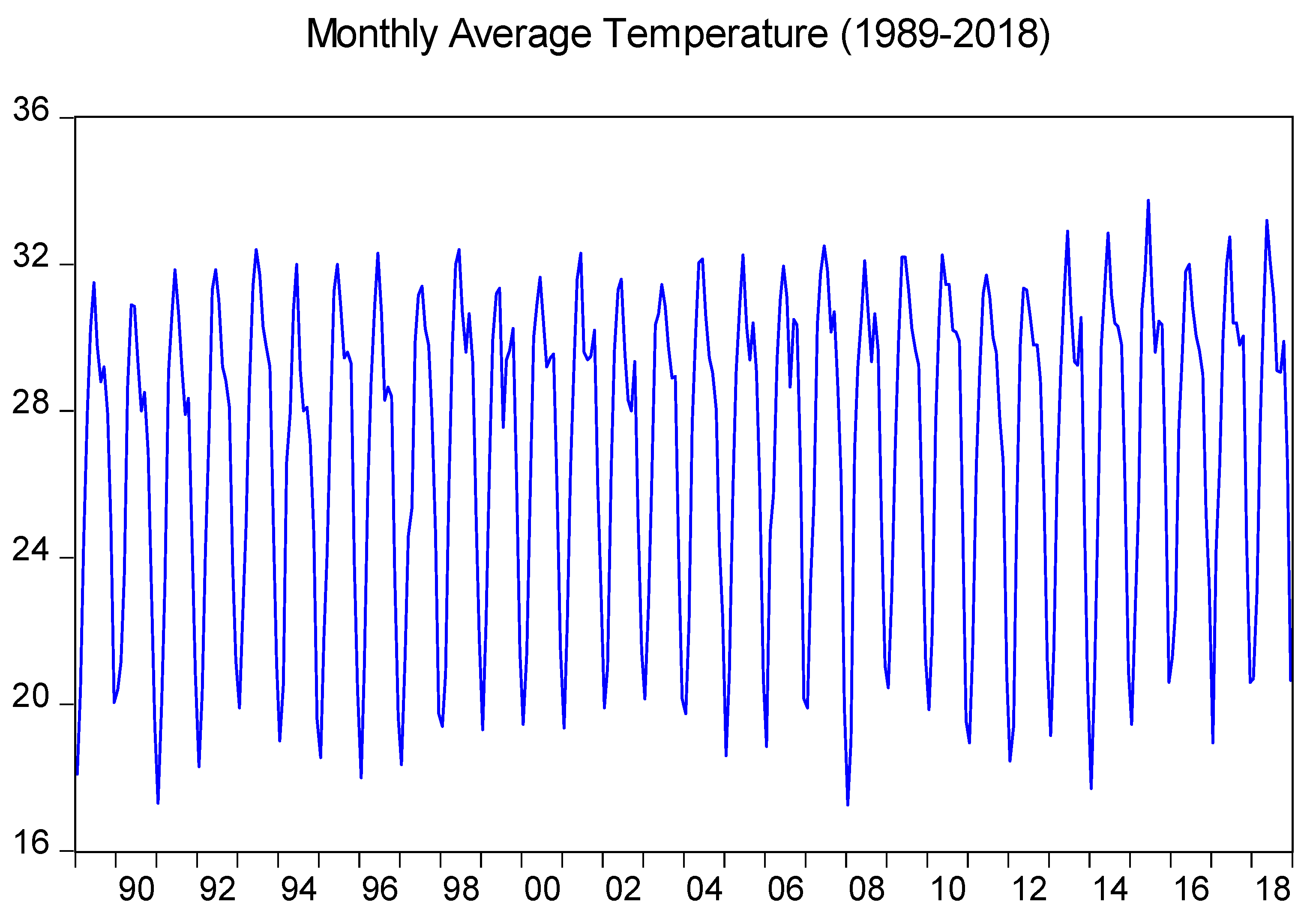
The monthly average temperature data of the Karachi station is used to study the behavior of time series. Figure 1 shows the plot of monthly average temperature. The varied peaks of the plot for the temperature series show the fluctuation of average monthly temperature.

3.2. Box-Jenkins Approach and ARIMA Models

The recorded daily mean temperature data were taken for the period from 1 January 1989 to 31 December 2018. Then the daily mean temperature data were converted into average monthly data (360 observations). Moreover, the average monthly data were separated into two sets, i.e., the training set (83.33%) that is consisted of 300 observations, and the validation set (16.67%) that consisted of 60 observations. After such divisions of the dataset, the modelling was performed using the Box–Jenkins approach by training data. For the purpose of checking whether data were stationary or not, the ADF test was conducted. In this way, it is easier to estimate and develop an appropriate model.

Corresponding values from the obtained results are displayed in

Table 2. The values of unit test of training dataset.

Null Hypothesis: Temp Is Stationary at First Differenced
ADF test statistic	−20.52576
Critical values
1% level	−3.452911
5% level	−2.871367
10% level	−2.572078

. This shows that the training dataset has been used from here onwards and computed the values.

From Table 2, one may infer that the null hypothesis about the series stationarity should not be rejected, as the ADF test shows critical values at less than 5% significance. From the consideration of the ADF test, the temperature series stationarity has been achieved.

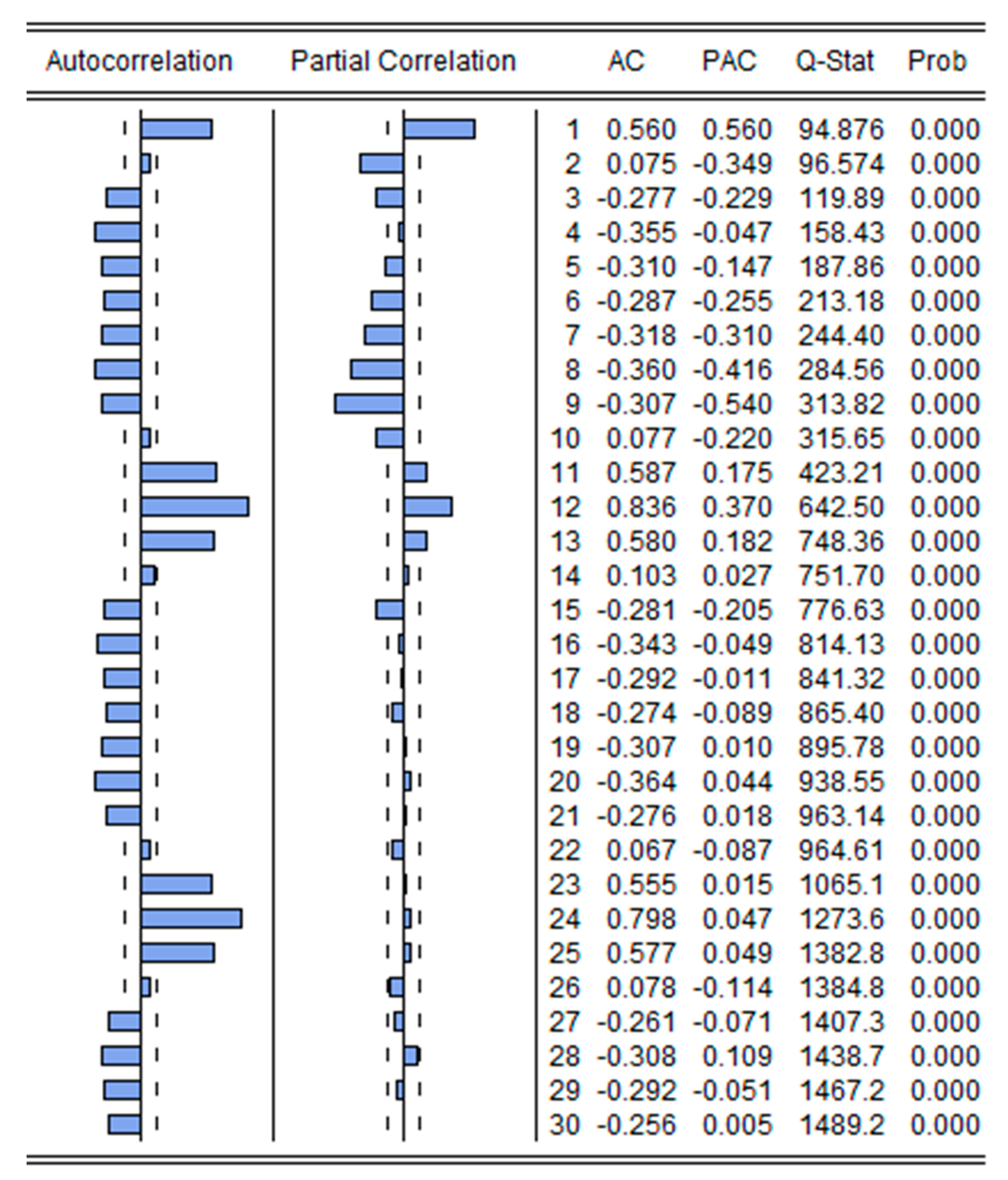
Once the time series stationarity is attained at the first difference, it is essential to examine the model’s ARIMA (p, 1, q) type, in which p and q are possible orders of AR and MA terms. Keeping in mind the dictum, the computations were performed for identification of suitable values of p and q, by ACF and PACF of the series, which is depicted through the Figure 2 below.

Given that when the tested PACF (of Figure 2) entails single significant autocorrelation at lag 1, it is hypothesized that the ARMA model to be fitted AR order should be 1. In this way, the subsequent models will be reflected as promising models to signify the original series. These models are: (i) ARIMA (1, 0, 0), (ii) ARIMA (1, 0, 1), (iii) ARIMA (1, 0, 2), (iv) ARIMA (2, 0, 0) (v) ARIMA (2, 0, 1) and (vi) ARIMA (2, 0, 2). A total of 24 ARIMA models have been run, and their respective AIC and BIC values are given in

Table 3. The computed values of fitted models.

Model	LogL	AIC *	BIC
(2, 4)(0, 0)	−538.334112	3.654409	3.753417
(4, 4)(0, 0)	−553.782575	3.771121	3.894882
(2, 3)(0, 0)	−563.708658	3.817449	3.904082
(3, 4)(0, 0)	−562.014711	3.819496	3.930881
(3, 3)(0, 0)	−563.695489	3.824050	3.923059
(3, 2)(0, 0)	−567.923813	3.845644	3.932277
(2, 2)(0, 0)	−576.457148	3.896034	3.970291
(4, 1)(0, 0)	−592.593820	4.010661	4.097293
(4, 3)(0, 0)	−591.931436	4.019608	4.130993
(3,1)(0,0)	−595.052507	4.020418	4.094674
(2, 1)(0, 0)	−596.255430	4.021775	4.083656
(4, 2)(0, 0)	−594.367551	4.029214	4.128223
(0, 4)(0, 0)	−616.377200	4.163058	4.237315
(1, 3)(0, 0)	−622.129350	4.201534	4.275791
(3, 0)(0, 0)	−642.047851	4.328079	4.389960
(4, 0)(0, 0)	−641.813930	4.333204	4.407460
(1, 4)(0, 0)	−642.802244	4.346503	4.433136
(1, 2)(0, 0)	−649.472671	4.377744	4.439624
(2, 0)(0, 0)	−650.957331	4.380985	4.430490
(0, 3)(0, 0)	−652.965777	4.401109	4.462989
(1, 0)(0, 0)	−670.071662	4.502152	4.539280
(0, 1)(0, 0)	−670.403286	4.504370	4.541498
(1, 1)(0, 0)	−713.790966	4.801277	4.850782
(0, 0)(0, 0)	−727.052156	4.876603	4.901355
(0, 2)(0, 0)	−725.735828	4.881176	4.930680

below.

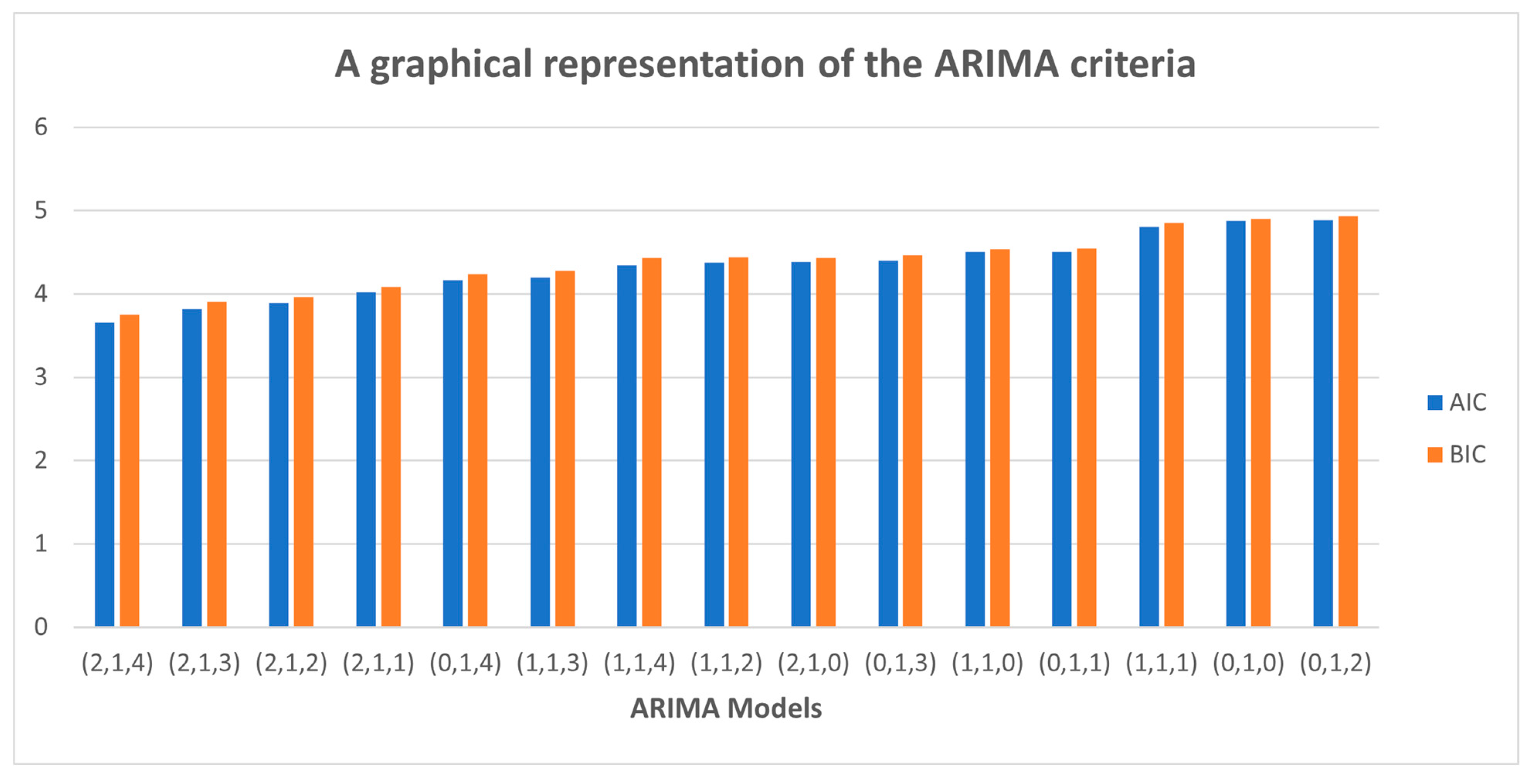
All models as displayed in Figure 3 are stationary at first difference, (2, 4)(0, 0) = (2, 1, 4). The results in Table 3 show that the model that has the maximum log likelihood estimates and the lowest AIC and BIC values was the ARIMA (2, 1, 4) model. Thus, it can be concluded that the best model for this study is ARIMA (2, 1, 4). Moreover, as is indicated in

Table 4. The estimated parameter of ARIMA (2, 1, 4) as the best fitted model.

Dependent Variable: D(AVGTEMP)
Variable	Coefficient	Std. Error	t-Statistic	Prob.
C	0.004238	0.001720	2.463441	0.0143
AR(1)	1.730060	0.003806	454.5069	0.0000
AR(2)	−0.997270	0.003574	−279.0121	0.0000
MA(1)	−2.108684	0.522888	−4.032767	0.0001
MA(2)	0.950378	0.524831	1.810826	0.0712
MA(3)	0.752699	0.358723	2.098277	0.0367
MA(4)	−0.594387	0.459242	−1.294280	0.1966
SIGMASQ	2.055260	0.572280	3.591351	0.0004
R-squared	0.728813	Mean dependent var		0.008528
Adjusted R-squared	0.722289	S.D. dependent var		2.757568
S.E. of regression	1.453190	Akaike info criterion		3.654408
Sum squared resid	614.5227	Schwarz criterion		3.753417
Log likelihood	−538.3341	Hannan–Quinn criter.		3.694036
F-statistic	111.7228	Durbin–Watson stat		1.740968
Prob(F-statistic)	0.000000
Inverted AR Roots	0.87 − 0.50i	0.87 + 0.50i
Inverted MA Roots	1.00	0.87 − 0.43i	0.87 + 0.43i	−0.63

, the constant term and AR(1) term are significant in our selected models.

3.3. Diagnostic Test of Fitted Model

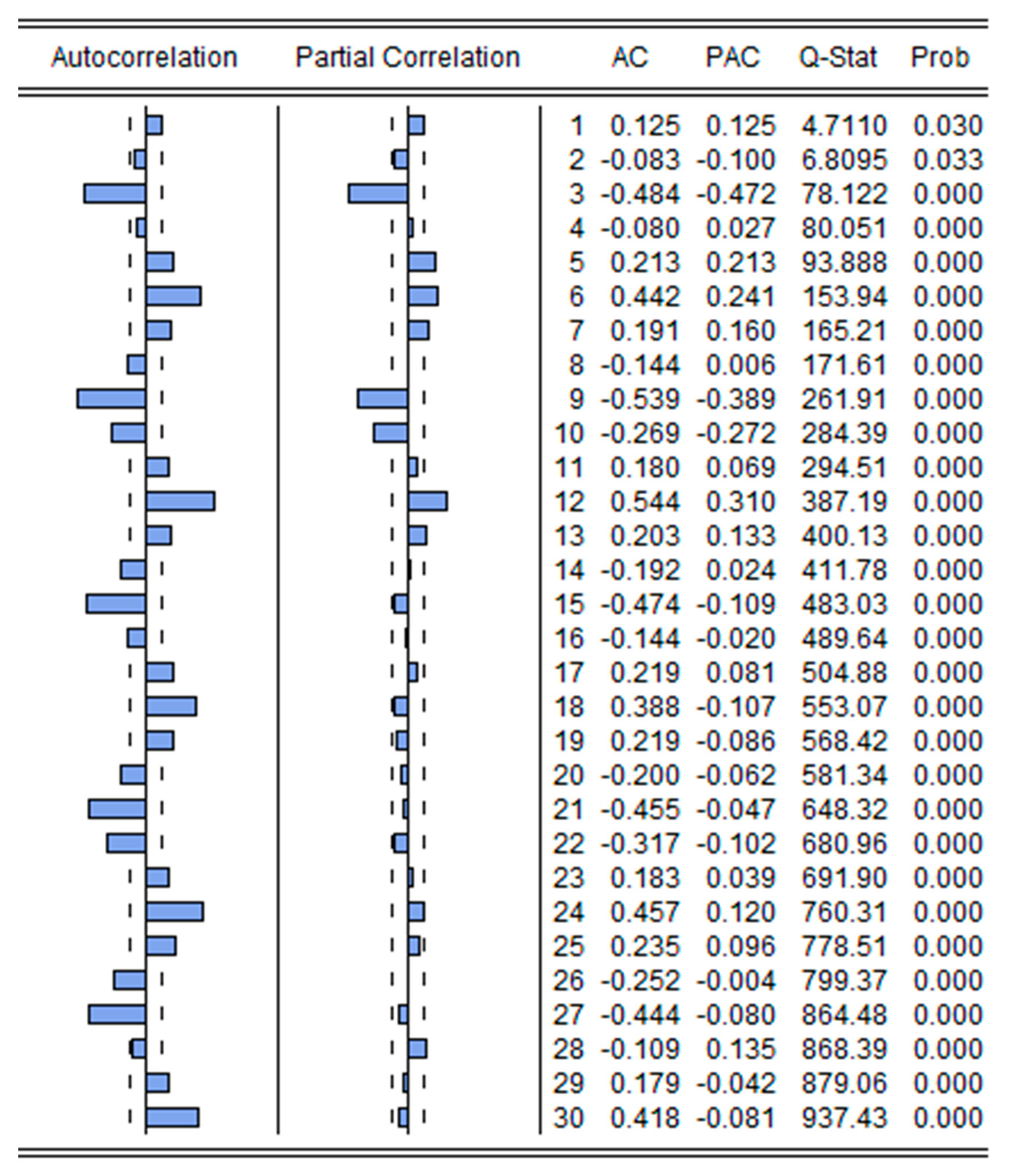
Randomness: The simplest form of a time series is a random process. In a random time series, the mean and variance of the observations fluctuate constantly and independently. In a sense, there is no pattern in a random time series. Moreover, the variance does not increase over periods of different observations. From Figure 4, it is clear that the residuals of the designated model are comparatively insignificant. Thus, the residuals of the fitted model should be considered as randomly distributed.

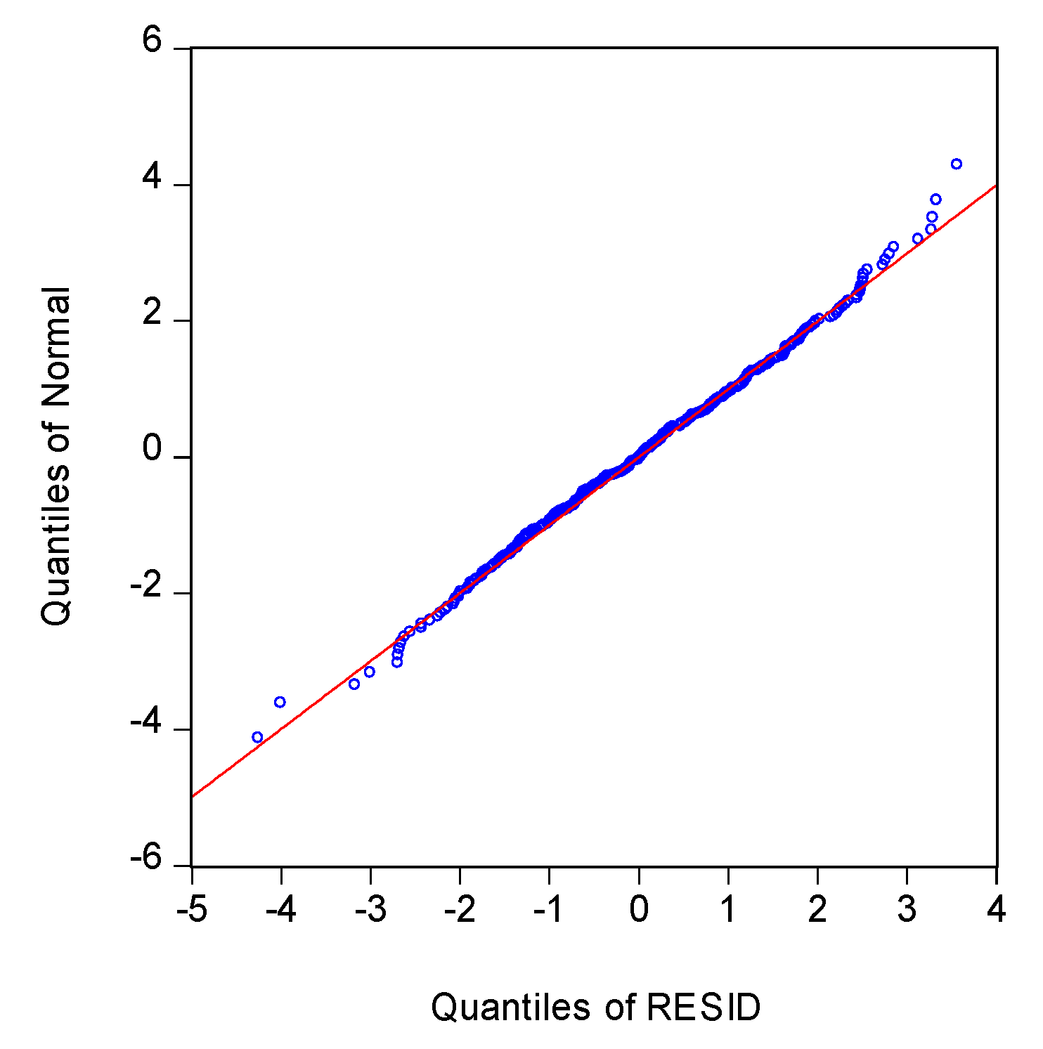
Normality: For the residuals of the selected model, normal probability plot technique was carried out for checking residuals, whether they are normal or not. In the following, the standard chart of residuals is plotted, which is also called Normal Probability Plot (NPP).

In Figure 5, it is shown that the respective Jarque–Bera statistic and p value are (JB = 1.364924, p = 0.505371). Accordingly, these respective values of JB and p confirm that the residual series is normally distributed.

The NPP reveals that the residuals are normal and there exist no outliers. This has also been confirmed by the Jarque–Bera test of normality. The JB statistic is 1.364924 with p value = 0.505371. The null hypothesis of the JB test is that the residuals are normally distributed. The p value for this test is higher than 5% level of significance, confirming that residuals are normal.

Testing the Heteroscedasticity: Through ARCH-LM test, the heteroscedasticity of the established model was observed. The obtained results in relation to heteroscedasticity of residuals are shown in

Table 5. Obtained results for checking heteroscedasticity of residuals.

ARCH-LM Test
F-statistic	0.805623	Prob	0.3701
Obs* R-squared	0.808876	Prob	0.3685

. The values show that the heteroscedasticity does not exist at 5% significance level (p = 0.368). The reason is that the associated p value relating to the F-statistic is much greater than 5% significance level.

In connection with the detailed analysis of residuals, it now becomes easier to confirm that the ARIMA (2, 1, 4) model as developed can fulfill all the diagnostic tests. Therefore, ARIMA (2, 1, 4) should be the best fitted model, which can be used to forecast the average monthly temperature of the Karachi region for the period 1989 to 2018.

3.4. Forecasting Temperature Using ARIMA (2, 1, 4)

It is better to confirm the model as developed with observed data (training set), as well as an independent dataset (validation set), instead of making forecasts. The forecasts’ errors of validation set of observed data are given below.

From

Table 6. Forecast performance of ARIMA (2, 1, 4) model.

Type of Data	Period	RMSE	MAE
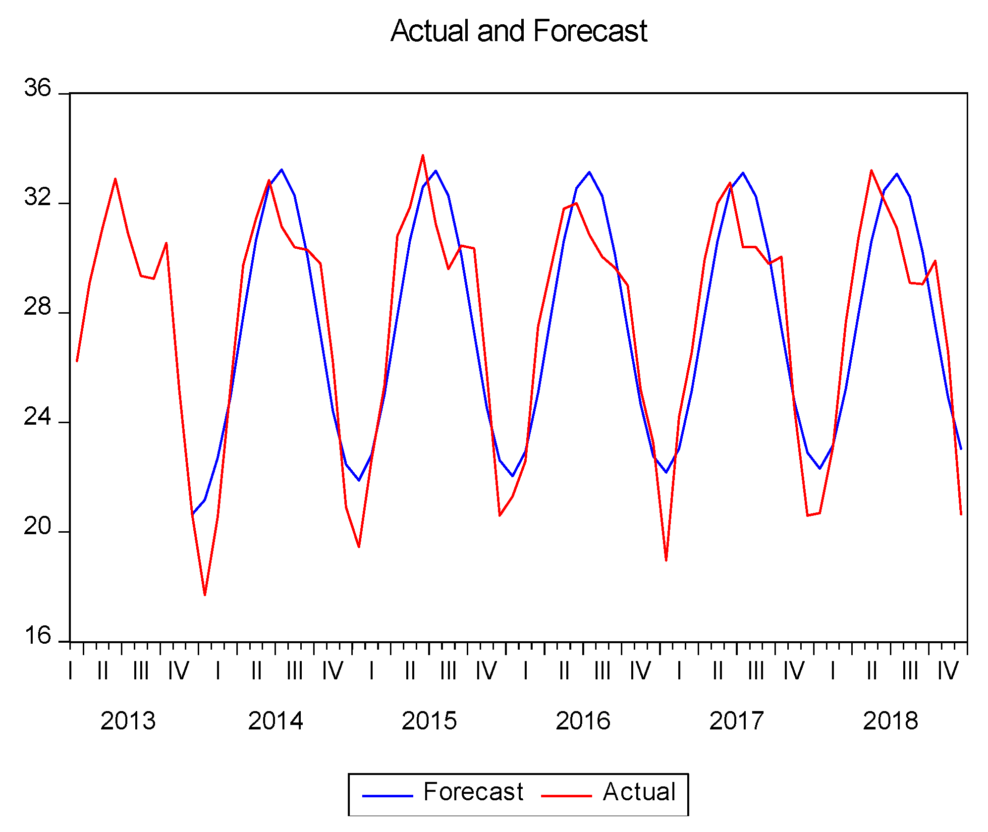
Validation set	2014–2018	1.848532	1.586789

, the values of RMSE (1.848532) and MAE (1.586789), respectively, show that ARIMA (2, 1, 4) is the best fitted model; the deviation shows within acceptable range. In Figure 6, the projected and observed values are depicted.

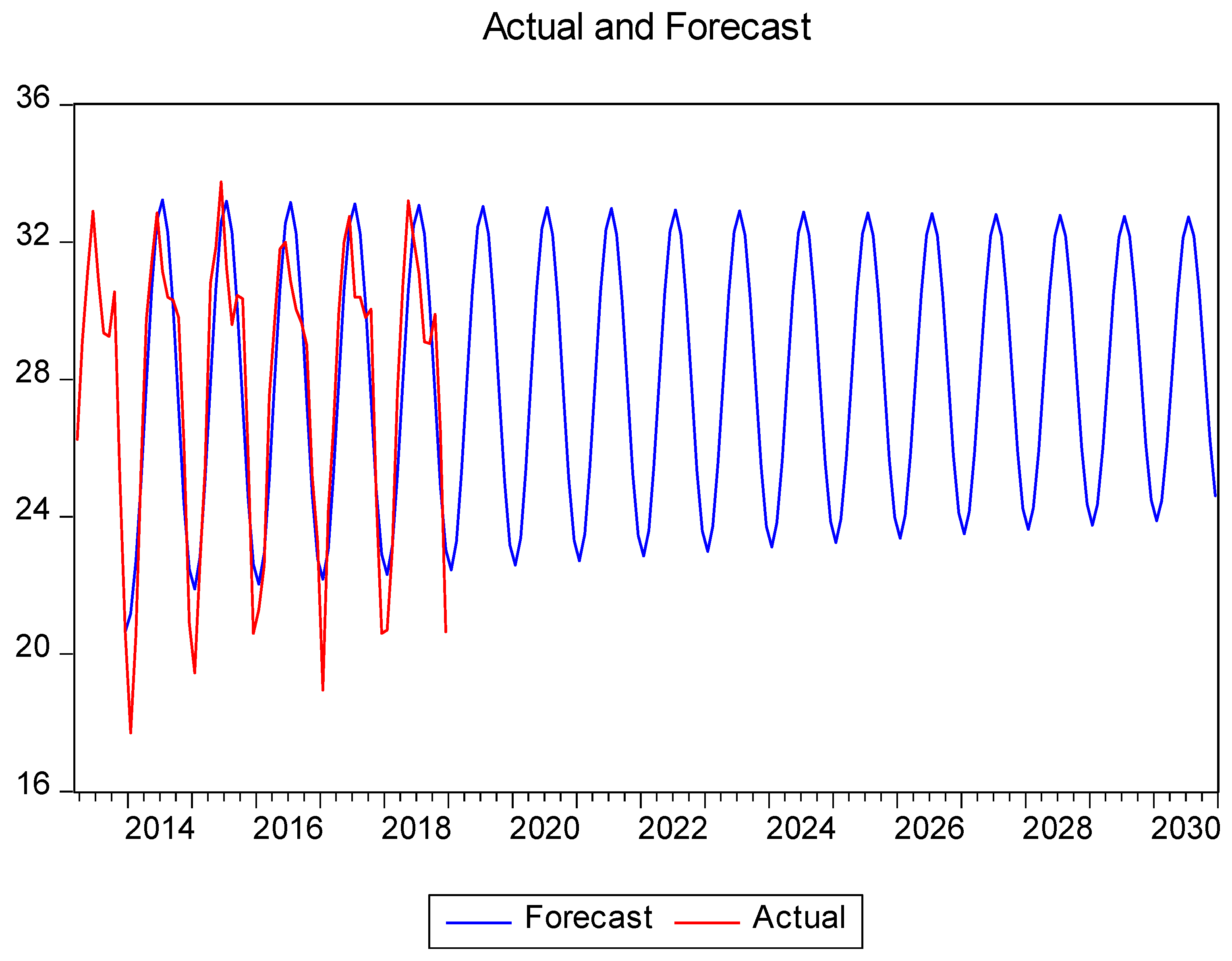
In the Figure 7, the temperature forecasts were generated based on the best-fitted ARIMA (2, 1, 4) model. It is clear from the generated values that the actual and forecasted values from 2014 to 2018 are close. There is no awkward type of fluctuation in the values of time series. This shows that the model seems to work accurately. The model’s accuracy is also confirmed by MAE and MAPE tests. Moreover, the out-of-sample forecasted values are also computed from January 2019 to December 2030, depicted in Figure 7.

4. Conclusions

Time series analysis is one of the important techniques in model building and forecasting of regional temperatures. In this study, the ARIMA technique was employed for building the model and forecasting the monthly average temperature of Karachi station from Jan 1989 to December 2018. The best fitting model for temperature was identified as ARIMA (2, 1, 4). The developed model was verified using diagnostic tests. It is confirmed that the residual series is normally distributed. RMSE and MAE for the validation set from the ARIMA (2, 1, 4) model show no deviation from the observed data, which should be considered as being within the acceptable range. Consequently, this developed model can help in determining possible future strategies related to the weather conditions of Karachi station. The ARCH-LM test was conducted to observe the heteroscedasticity of the developed model. The results regarding the heteroscedasticity of residuals do not show the existence of heteroscedasticity at 5% significance level. This work can further be augmented with more robust modeling techniques in future endeavors related to regional warming and temperature variability on the regional scale.