Correlation Structure and Co-Movement of Hunan Province’s Air Pollution: Evidence from the Multiscale Temporal Networks

Abstract

In recent years, air pollution has become one of the main factors harming the livable environment for human beings. Governments have recognized the importance of controlling air pollution and reached a consensus that regional joint control of air pollution is an effective means of dealing with environmental degradation. In this work, we focus on the impact of fine particulate matter and nitrogen compounds on the air quality of 14 prefecture-level cities in China’s Hunan Province using the insights of complex networks, and further propose a joint treatment scheme for these two pollutants. Multiscale temporal networks are constructed based on the height cross-correlation coefficient, which allows us to assess the variable network structures concerning different time scales. We use four network properties to assess the network structures for the pollutants. Through the Jensen-Shannon divergence of the probability distribution of these network attributes, it is found that NO₂ affects AQI more in a short time interval than in a longer time interval. The correlation of both NO₂ and PM_2.5 among the 14 cities in about 15 days can best reflect the air quality in Hunan Province. In addition, instead of NO₂, PM_2.5 has become the culprit of air pollution in Hunan Province. The co-movement of the pollutants among the 14 cities is significant. The co-movement of the PM_2.5 pollutants can last 45 days, while that of NO₂ pollutants will gradually decrease over time. Furthermore, by using spectral clustering based on the network node correlation, we classify the 14 cities into five regions and two regions for PM_2.5 and NO₂, respectively. It provides a feasible implementation guide for the environmental governance of regional cooperation.

1. Introduction

Environmental pollution has become a worldwide issue. The problem of air pollution is particularly prominent because it is directly related to the respiratory health of all people on earth. More and more governments have realized the importance of managing air pollution and actively introduced a series of countermeasures [1].

In the work of controlling air pollution, it is an effective prerequisite to detect the laws behind the monitored environmental data through statistical analysis. With the advancement of modern statistical methods, it is of great importance to assess the trend and propagation characteristics of smog from a statistical point of view [2,3,4]. A lot of research shows that the study of the correlation between pollutants and meteorological factors, as well as other pollutants, helps explore the formation and spread of pollution. Researchers such as Shi [5] have investigated the relationship between temperature, rainfall, PM₁₀ (an inhalable particle with a diameter ≤ 10 μm), and ambient dioxins concentration in Hong Kong city. Liu et al. [6] found that the air pollutants at most stations in China were significantly negatively correlated with wind speed, precipitation, and relative humidity, but positively correlated with atmospheric pressure. Wang and Fan [7] proposed a coupling correlation analysis for detecting the coupling of six pollutants in Beijing’s air quality index (AQI) system. Long et al. [8] investigated the impact of rainfall and wind speed on the air pollutants in the Sichuan Basin of China by using Pearson’s correlation coefficient. Using the detrend multiple cross-correlation coefficient [9], Wang et al. [10] investigated the impact of four typical air pollutants of PM_2.5 (fine particulate matter diameter ≤ 2.5 μm), PM₁₀, NO₂, and CO on the AQI of Beijing city. In addition, many meaningful works have focused on the correlation between the neighboring regions, which is conducive to investigating the propagation behavior and exploring the diffusion source [1,11,12,13]. Among them, Wang et al. [11] developed a new time-lagged cross-correlation coefficient to find there are varying degrees of time-lagged correlation of PM_2.5 series between Beijing, Tianjin, Baoding, and Zhangjiakou in North China. Chen et al. [12] evaluated Beijing air quality at the local and regional scale by using weighted cross-correlogram spectral matching technology. To some extent, these works allow us to assess the interaction of the pollutants among different cities and confirm the co-movement of regional air pollution. However, the information obtained from the correlation analysis of the pollutant concentration series is limited, since the static structure (which can be regarded as a ‘low-dimension’ feature) of the series itself cannot express the dynamic evolution process of the pollution concentration sequence, which must be excavated by the ‘high-dimension’ tools.

As one of the most important tools to explore our real world in the 21st century, complex networks [14] build a bridge between the object phenomena in the world and rational scientific research. The complex network theory brings a new perspective to uncover the rich information of real systems. In practice, mapping time series to the network helps to uncover the dynamic structure and evolution law while the simple correlation analysis is difficult to complete. Generally, there are three classes of methods to translate time series into the network, namely, proximity networks [15,16,17], visible graph networks [18,19], and transition networks [20,21]. Among them, as one of the proximity networks, the correlation network [15] is the simplest which makes use of correlation relationships between different parts of a dynamical system’s trajectory [22]. Scientists in various fields apply these tools to re-understand the world and gradually master the laws behind the phenomenon [22]. In the past 20 years, a great number of new network methods have been proposed to deal with various critical difficulties or real problems in different fields, including problems of air pollution [23,24,25,26,27]. Among them, Song et al. [23] exploited a network statistical model to assess the PM_2.5 concentration in the region of Jing-Jin-Ji of North China. Plocoste et al. [24] applied a multiplex visibility graphs network to find the effect of wet scavenging by rainfall on PM₁₀ of the Guadeloupe archipelago. Zhang et al. [25] developed a novel multiscale time-lagged networks framework to investigate the interaction of air pollution among nine neighboring cities in North China. Dai and Zhou [26] applied the planar maximally filtered graph network to investigate the correlation among the six pollutants in 350 Chinese cities from temporal and spatial perspectives.

The successful application of the method of the complex networks of environmental pollution monitoring provided the experience to study the interaction of regional air pollution, which motivated us to use this technique to probe into the co-movement of different pollutants among the local regions in Hunan Province. This area is one of the core regions in Central China’s Rising Strategy, whose economy is on a rapid growth track, while it is simultaneously accompanied by deteriorating air quality. Due to its special geographical location and climate environment, the air pollutants in the atmospheric circulation for Hunan Province are difficult to dissipate. The source of air pollution mainly stems from industrial pollution, vehicle exhaust emissions, and urban construction dust. According to the Bulletin of the Second National Pollution Source Census in Hunan Province [28], which was jointly released by the Departments of Ecological Environment, the Bureau of Statistics, and Agriculture and Rural Affairs of Hunan Province on 9 December 2020, multiple pollution sources cause the air pollution in Hunan Province. Overall, there were 228,000 tons of sulfur dioxide, 567,500 tons of nitrogen oxides, 597,600 tons of particulate matter, and 294,300 tons of volatile organic compounds in the emission of air pollutants in 2017. Against this background, we focus on the statistical properties of the two main pollutants, namely, NO₂ and PM_2.5, and seek to compare their impact on Hunan’s air quality system. In addition, we try to aggregate the 14 cities of Hunan Province into several regions for joint governance of environmental pollution among the cities.

We emphasize that this work is conducted based on the statistical perspective. Multiscale correlation analysis of the pollutants among the 14 cities will provide evidence for the observed pollution phenomena (such as PM_2.5 being the main air pollution of Hunan Province). Network properties analysis will uncover the different network structures of the two pollutants at different time scales. Spectral clustering will help to classify the 14 cities into several regions for jointly governing the air pollutants. The findings may provide a theoretical reference for further studies on the dynamics of the pollutants over time and interregional joint treatment of air pollution.

2. Materials and Methods

2.1. Height Cross-Correlation Analysis (HXA)

To investigate the cross-correlation of the air pollutant series between every pair of cities at different time scales, in this work, we apply height cross-correlation analysis (HXA) [29] to calculate the multiscale cross-correlation coefficient [30,31]. The method of HXA originated from the multi-affine analysis [32] which was widely used to deal with univariate time series with statistical self-similarity. With the same idea, the HXA is designed to analyze the cross-correlation between two fractal series, which is similar to the well-known detrended cross-correlation analysis (DCCA) [33]. However, in some ways it is quite different from the DCCA and does not need a fitting process in the local interval, while the DCCA does. Thus, its calculation speed is faster. For the two series {x_t} and {y_t}, t = 1, 2, …, N. N is their sampling length. Define the profile series as

$$X(t)={\displaystyle \sum _{i=1}^t\left[x_i-〈x〉\right]},Y(t)={\displaystyle \sum _{i=1}^t\left[y_i-〈y〉\right]},$$

(1)

where $〈x〉$ and $〈y〉$ denote the average values of series {x_t} and {y_t} over the entire time sampling range, respectively. This step is necessary to avoid the influence of non-stationary measures on the original series. Then, the mutual increment between the profile X(t) and Y(t) with the interval L is determined by Equation (2), which may be regarded as the covariance of time lag L,

$$F_{xy}^{}(L)=\frac{1}{N-L}{\displaystyle \sum _{t=1}^{N-L}[X(t)-X(t+L)]\cdot [Y(t)-Y(t+L)]}$$

(2)

When x_t = y_t, the above covariance degenerates to the variance of {x_t} as

$$F_x^{}(L)=\frac{1}{N-L}{\displaystyle \sum _{t=1}^{N-L}{[X(t)-X(t+L)]}^2}$$

(3)

F_x(L) and F_xy(L) characterize the fluctuation information of the series {x_t} itself and two series between {x_t} and {y_t} with lag L, respectively. To qualify the strength of cross-correlation between the {x_t} and {y_t}, like Pearson’s correlation coefficient, the HXA-based cross-correlation coefficient can be defined as,

$$\rho (L)=\frac{F_{xy}^2(L)}{\sqrt{F_{xx}^2(L)F_{yy}^2(L)}}=\frac{{\displaystyle {\sum }_{t=1}^{N-L}[X(t)-X(t+L)]\cdot [Y(t)-Y(t+L)]}}{{\displaystyle {\sum }_{t=1}^{N-L}{[X(t)-X(t+L)]}^2}}$$

(4)

The ρ(L) can quantitatively describe the cross-correlation between the two series at varying scales. The ρ(L) is dimensionless with $-1\le \rho (L)\le 1$.

To test the significance of the ρ(L) at a given scale L, we use the Monte Carlo method to calculate the critical value [31]. To do so, 10,000 repetitions of shuffled AQI/PM_2.5/NO₂ series between two cities are employed to compute the ρ(L) at scale L. Then, the probability density function (PDF) is obtained, which is expected to be a normal distribution according to the central limit theorem. Given a significance level α (in this work, we took α = 0.05), let the integral of PDF between −ρ₀(L) and ρ₀(L) be equal to 1 − α, then we can obtain the ρ₀(L), which is just the critical value of ρ(L) at scale L. The area above the ρ₀(L) indicates statistically significant cross-correlations between two series, while the area below ρ₀(L) would suggest insignificant cross-correlations [34].

2.2. Complex Networks Construction and Properties

2.2.1. Network Construction

For the multivariable series, the simplest idea to construct a complex network involves using the correlation between every pair of series [15]—namely, each air pollutant factor series is considered as a network node (N), and the correlation between two pairs of time series is taken as the basis for edge (E) connection. In this spirit, the HXA-based cross-correlation coefficient given by Equation (4) is employed here to construct the network edge. According to the statistical test of ρ(L), for a given scale L, we use Equation (5) to determine the edge weight (W) ω_ij between the nodes i and j. Then, a family of AQI/PM_2.5/NO₂ networks G = (N, E, W, L) of 14 cities in Hunan Province can be constructed. They are all undirected weighted networks.

$${\omega }_{ij}(L)=\left\{\begin{array}{cc}{\rho }_{ij}(L)& {\rho }_{ij}(L)>{\rho }_0(L)\\ 0& \mathrm{otherwise}\end{array}\right.$$

(5)

2.2.2. Network Topological Properties

To uncover the proposed dynamical structure of the AQI/PM_2.5/NO₂ networks with varying scales, four topological properties [14] are employed for our consideration, namely, node strength, clustering coefficient, average path length, and graph density, where the former three is for every node and the latter is for characterizing the global feature of the network.

(1)

Node strength

In the weighted network, the strength of node i is defined as the sum of the weights of node i and all its neighbors [14], given by,

$$NS(i)={\displaystyle \sum _{j\in V(i)}{\omega }_{ij}},$$

(6)

where V(i) represents a set consisting of all nodes connected to node i. ω_ij is the edge weight value given by Equation (5). Then, the average node strength of the network is

$$〈NS〉=\frac{1}{N}{\displaystyle \sum _{i=1}^{N}NS(i)},$$

(7)

where N is the number of nodes in our network. Here, N = 14, the same as below.

(2)

Clustering coefficient

The clustering coefficient describes the group nature between the node neighbors, which expresses the medium-range topological information of a node in the corresponding network. There are several definitions of the clustering coefficient for the weighted network [35,36,37]. In this work, we utilized the definition introduced by Holme et al. [36], as shown below:

$$CC(i)=\frac{{\displaystyle \sum _{j\ne k}{\omega }_{ij}\cdot {\omega }_{ik}\cdot {\omega }_{jk}}}{\underset{j}{\max }({\omega }_{ij}){\displaystyle \sum _{j\ne k}{\omega }_{ij}{\omega }_{ik}}},$$

(8)

where ω_ij is the edge weight connecting the nodes i and j. Consequently, the average clustering coefficient over the network is determined by

$$〈CC〉=\frac{1}{N}{\displaystyle \sum _{i=1}^{N}CC(i)}.$$

(9)

(3)

Average path length

The shortest path between two nodes i and j in an unweighted network refers to the path connecting the two nodes with the least number of sides. The distance between nodes i and j is defined as the number of edges on the shortest path connecting the two nodes. In the weighted network, the shortest path between two nodes refers to the path with the smallest sum of weights (heterogeneous network) or reciprocal sum of weights (homogeneous network) connecting the edges of these two nodes [38]. The path length of node i to j is the sum of the edge weights on the shortest path connecting the nodes i and j. In this work, we used the Floyd algorithm [39] to calculate the path length between every two nodes. Since the homogeneous network is considered in our work, we took 1/ω_ij in the Floyd algorithm to compute the path length of the node i to j. The average path length of each node refers to the average distance from the node to all nodes connected to it, determined by

$$APL(i)=\frac{1}{\#V(i)}{\displaystyle \sum _{j\in V(i)}floyd(\frac{1}{{\omega }_{ij}})},$$

(10)

where #V(i) denotes the number of nodes connected to node i. Hence, the average of average path length over the network is:

$$〈APL〉=\frac{1}{N}{\displaystyle \sum _{i=1}^{N}APL(i)}.$$

(11)

(4)

Graph Density

Graph density [14] refers to the closeness of communication between nodes in a network, which can be used to measure the interaction degree of pollutants between stations. The value of graph density is limited in the range of [0,1]. The higher graph density means that the nodes are more closely connected. The calculation of the directed network’s graph density is as follows:

$$GD=\frac{M}{N(N-1)},$$

(12)

where M is the number of edges in the network.

2.3. Jensen-Shannon Divergence

In information theory, Kullback–Leibler (K-L) divergence and Jensen-Shannon (J-S) divergence [40] are used to measure the difference in probability distribution between two signals. The larger the value is, the more obvious the difference is expected. K-L divergence is the fact the relative entropy, whose discrete form is defined by:

$$D_{K-L}(P\Vert Q)={\displaystyle \sum p(x){\log }_2\frac{p(x)}{q(x)}},$$

(13)

where P and Q are two probability distributions of random variable x. Apparently, $D_{K-L}(P\Vert Q)\ge 0$. The two distribution is identical in the case of $D_{K-L}(P\Vert Q)=0$. In general, $D_{K-L}(P\Vert Q)\ne D_{K-L}(Q\Vert P)$, implying the K-L divergence is not symmetrical. To make up for this defect, J-S divergence is designed to be regarded as the ‘distance’ between two probability distributions, thus, it has symmetry. In addition, the J-S divergence is dimensionless with a range [0,1], which is defined by:

$$D_{J-S}(P\Vert Q)=\frac{1}{2}{D}_{K-L}\left(p\Vert \frac{p(x)+q(x)}{2}\right)+\frac{1}{2}{D}_{K-L}\left(q\Vert \frac{p(x)+q(x)}{2}\right).$$

(14)

In the following analysis, we utilized the J-S divergence to examine the probability distribution’s difference of the cross-correlation coefficient and network topological properties between AQI and the two pollutants.

2.4. Spectral Clustering

Spectral clustering is a clustering algorithm with superior performance that has prevailed over the last 20 years. It derives new features of clustering objects through matrix spectral analysis theory and utilizes the new features to cluster original data. It is simple to implement and has the advantage of identifying clustering for non-convex distribution [41]. For our network G = (N, E, W, L), and the edge weight ω_ij is the cross-correlation coefficient determined by Equation (5). The larger ω_ij is, the closer the nodes I and j are. In this regard, the distance between the nodes i and j should be defined by:

$$d_L(i,j)=\frac{1}{{\omega }_{ij}(L)}.$$

(15)

Then, we use the Gaussian kernel function to measure the similarity of the nodes i and j. Here, we weigh the time scales to synthesize the influence of different scales on similarity. Hence the similarity is given by

$$w_{ij}=\exp \left(-\frac{{\displaystyle {\sum }_L{\alpha }_L\cdot d_L{(i,j)}^2}}{2{\sigma }^2}\right),$$

(16)

where σ is a parameter and taking 1 in this work. α_L is the weight of the distance at the time scale L, which is determined by

$${\alpha }_L=\max \left\{0, \frac{\rho (L)-{\rho }_0(L)}{{\displaystyle {\sum }_L{[\rho (L)-{\rho }_0(L)]}^{+}}}\right\},$$

(17)

where ${[\rho (L)-{\rho }_0(L)]}^{+}=\max \{0,\rho (L)-{\rho }_0(L)\}$. So far, the adjacency matrix W = (w_ij) is obtained. Furthermore, define D as a diagonal matrix with the element $d_i={\displaystyle {\sum }_j{w}_{ij}}$. Thus, the Laplace matrix is calculated by

L = D − W.

(18)

Next, normalize the Laplace matrix L as,

$$L^{*}=D^{-\frac{1}{2}}L{D}^{\frac{1}{2}}.$$

(19)

Consequently, calculate the K eigenvectors corresponding to the K least eigenvalues of L^* and form them to the characteristic matrix, which is an input of clustering. K-means clustering is considered for this purpose.

2.5. Method Discussion

In this work, we utilize the above methods to conduct our study. In practice, an HXA-based coefficient is a useful tool to quantitatively evaluate the correlation of the pollutant concentration series between two cities. Network analysis helps us uncover rich information about the AQI and the two pollutants while traditional time series analysis cannot. J-S divergence is employed to compare the difference of PDF of the statistical properties between AQI and the two pollutants. Finally, we apply spectral clustering to aggregate the studied cities into several regions for joint governance of environmental pollution among the cities. It is worth noting that none of the above methods is unique to our studied purpose. However, they are common methods and easy to implement.

3. Case Study

3.1. Data Description

Hunan Province (24.7° N~30.1° N, 108.8° E~114.2° E) is located in the transition zone from Yunnan and Guizhou Plateau to the Jiangnan hills, and from the Nanling Mountains to the Jianghan Plain. It is surrounded by mountains on three sides and stretches across the Yangtze River and the Pearl River. It is a subtropical monsoon climate. With the implementation of the Plan for the Rise of Central China and the acceleration of urbanization, the industry has developed rapidly, while the level of air pollution is increasing. In addition, the imbalance of regional development leads to different types and levels of air pollution, which increases the difficulty of air pollution control. In general, different linkage behavior in neighboring cities has been observed for different pollutants. Moreover, in our previous work, we have found that six air pollutants (PM_2.5, PM₁₀, SO₂, CO, NO₂, and O₃) have significantly different effects on the air quality index (AQI) [6,9,42]. Specifically, the correlation between the AQI and fine particulate matter (PM_2.5 and PM₁₀) is stronger than that of AQI and traditional pollutants (NO₂ and SO₂), implying that urban pollution has been gradually transformed into fine particulate matter pollution from traditional industrial waste gas pollution such as nitrogen compounds and sulfide [42]. In this work, we focus on the regional similarity of air pollution and co-movement among the 14 cities (Changde [CD], Changsha [CS], Chengzhou [CZ], Huaihua [HH], Hengyang [HY], Loudi [LD], Shaoyang [SY], Xiangtan [XT], Xiangxi [XX], Yiyang [YI], Yueyang [YU], Yongzhou [YZ], Zhangjiajie [ZJ], Zhuzhou [ZZ]) in Hunan Province from the perspective of a complex network. To do so, we chose the time series of AQI and two pollutants, PM_2.5 and NO₂, for consideration. The dataset included daily average data recorded from 1 December 2015 to 30 November 2018 (1096 observation samples for each series), downloaded from http://www.tianqihoubao.com/aqi/ (accessed on 19 June 2021). The mean values and standard deviation over the sampling range are listed in

Table 1. Descriptive statistics of AQI, PM_2.5, and NO₂ of 14 cities of Hunan Province.

City Name	Location	AQI			PM2.5 (μg/m³)			NO2 (mg/m3)
		Mean(Std)	K	S	Mean(Std)	K	S	Mean(Std)	K	S
CD	29.02° N, 111.51° E	73.42 (37.67)	9.86	1.91	48.01 (32.32)	11.69	2.04	19.37 (10.59)	4.13	1.05
CS	28.12° N, 112.59° E	75.91 (39.62)	6.99	1.67	49.65 (33.41)	7.56	1.78	34.52 (16.14)	3.67	0.99
CZ	25.46° N, 113.02° E	61.46 (28.40)	6.86	1.53	35.45 (25.22)	6.42	1.55	24.50 (9.88)	3.63	0.87
HH	27.33° N, 109.58° E	65.71 (27.01)	5.48	1.33	37.39 (25.07)	4.75	1.30	15.65 (9.06)	4.52	1.28
HY	26.53° N, 112.37° E	70.65 (38.10)	6.24	1.53	46.77 (32.12)	7.08	1.63	27.13 (12.84)	4.00	1.12
LD	27.44° N, 111.59° E	62.11 (28.09)	12.11	1.95	37.57 (23.34)	16.35	2.49	19.23 (9.17)	4.38	1.17
SY	27.14° N, 111.28° E	72.29 (38.57)	8.84	1.90	49.12 (32.80)	15.72	2.43	19.83 (10.04)	4.96	1.32
XT	27.52° N, 112.53° E	74.90 (38.27)	6.03	1.53	48.48 (32.25)	6.22	1.59	32.05 (14.98)	3.72	1.02
XX	28.18° N, 109.43° E	57.40 (25.49)	6.03	1.29	34.89 (21.51)	5.83	1.42	14.32 (6.92)	5.75	1.38
YI	28.36° N, 112.20° E	68.60 (30.63)	8.95	1.83	40.04 (26.92)	8.67	1.92	24.51 (12.07)	3.51	0.98
YU	29.22° N, 113.06° E	71.05 (32.33)	16.65	2.19	46.20 (28.28)	39.56	3.48	22.29 (10.38)	3.26	0.80
YZ	26.13° N, 111.37° E	66.04 (31.86)	6.27	1.49	43.95 (26.54)	5.92	1.42	21.59 (11.03)	5.27	1.31
ZJ	29.08° N, 110.29° E	62.49 (30.16)	8.89	1.99	37.20 (26.63)	7.58	1.85	17.14 (6.20)	5.69	1.30
ZZ	27.51° N, 113.09° E	72.19 (38.71)	7.98	1.81	47.07 (32.54)	9.78	2.08	30.90 (13.79)	3.34	0.80

Tips: the number in the parentheses beside the mean value is the standard deviation. The letter K denotes kurtosis and S denotes skewness, respectively.

.

3.2. Correlation Analysis

To assess the correlation of AQI as well as PM_2.5 and NO₂ among the 14 cities from different time scales, we set 15 time scales (L in Equations (2)–(4) refers to time interval at time points of t and t+L) from 3 days to 45 days, with a step size of 3 days. The calculation of correlations in different time intervals helps access the seasonal trend (cycle) in the studied pollutants’ time series. Firstly, we calculated the multiscale ρ(L) for every pair of cities (91 pairs in all) according to Equation (4), as shown in Figure 1, in which the critical values (black dotted line) at every time scale is also shown. For the series AQI (Figure 1a) and PM_2.5 (Figure 1b), the ρ(L) of the 91 pairs of cities are larger than the critical value at every time scale, which suggests there is a strong co-movement of the fine particulate pollution among the 14 cities. However, the ρ(L) of many pairs of cites is below the black dotted line shown in Figure 1c, which means the NO₂’s correlation among the 14 cities cannot be significant at some scales. It explains that NO₂’s emissions are unbalanced in the Hunan Province. As mentioned above, NO₂ is mainly produced by industrial production, while the regional economic development in Hunan Province is proportional to the local industrial development. Therefore, the NO₂ pollution level is proportional to economic development. As expected, and seen in Table 1, the regions worst affected by NO₂ pollution are located in the cities with relatively developed economy, such as Changsha (CS, the provincial capital of Hunan Province), Xiangtan (XT), and Zhuzhou (ZZ). These three cities are now in the process of integration. The average ρ(L) of each pair of the three cities over all given scales is 0.8135. In contrast, the three cities with the least pollution were Xiangxi (XX), Zhangjiajie (ZJ), and Huaihua (HH). The average ρ(L) of each pair of the three cities over all given scales was 0.3024, which is less than that between the former three cities apparently. In contrast, the PM_2.5 pollution prevails in all the cities. The average ρ(L) of each pair of the 14 cities over all given scales reached 0.9169.

To more clearly show the influence of ρ(L) on the edge weight for the PM_2.5’s and NO₂’s network, we draw the probability density function (PDF) of the ω(L) for the three environmental factors at small (L = 6 d), medium (L = 21 d) and large (L = 45 d) scales in the left panel of Figure 2. To better visualize the different profiles of the ω(L)’s distributions, all histograms are rescaled so that the peak value is 1. The peak of the three PDFs moves to the right as the scale increases. However, the PDF shape of the AQI and PM_2.5 are so consistent, that they are quite different from that of NO₂. The J-S divergence calculated for the AQI versus PM_2.5 and AQI versus NO₂ confirms this, as shown in the right panel of Figure 2. The J-S divergence between the AQI and PM_2.5 closes to zero at every given scale, which is in agreement with the result obtained from the cross-sample entropy [42]. In contrast, the J-S divergence between the AQI and NO₂ increases concerning the time scales, which is explained by the difference in the PDF between the AQI and NO₂ increases over time. It indicates that NO₂ affects AQI more in short-time intervals than in long-time intervals. Meanwhile, the fact that it is significantly far from zero indicates that the propagation behavior of NO₂ among the 14 cities in Hunan Province is dissimilar to that of PM_2.5, especially at larger time scales. This finding indicates that PM_2.5 has replaced NO₂ as the main culprit of air pollution in Hunan Province.

3.3. Network Structural Analysis

Next, according to the rule given by Equation (5), the networks are constructed for the AQI as well as the two pollutants respectively, at the given time scales. It is easy to know that the networks of AQI and PM_2.5 are fully connected because the correlation of all pairs of cities is significant as shown in Figure 1a,b. In contrast, Figure 1c illustrates the partial of correlation coefficients located below the critical line, demonstrating that the network of NO₂ is not fully connected. To show this, take networks at the above three given scales as examples, as shown in Figure 3. The number of edges in the network of L = 6d is more than that in the network of L = 21d, while the latter is more than that in the network of L = 45d. Another important finding is that the degree and strength are out-of-balance among the 14 nodes for the NO_2′s network. The difference may help distinguish them and further cluster them for regional joint pollution control. This point will be elaborated on in Section 3.4.

In the following section, we investigate the network’s topological properties regarding three environmental factors. In the left panel of Figure 4, we show the PDF of node strength, clustering coefficients, and average path length of the AQI, PM_2.5, and NO₂ networks by integrating all scale information. Similarly to the left panel of Figure 3, all histograms are rescaled so that the peak value is 1. Unsurprisingly, the PDF shapes of the three topological properties of the AQI’s network are highly consistent with those of the PM_2.5, while they are different from that of NO₂. The consistency of these network attributes between AQI and PM_2.5 explains that the main factor affecting AQI in Hunan Province from 2015 to 2018 is PM_2.5 rather than NO₂. Seen from the figure, some findings can be concluded as follows. Firstly, the node strength of PM_2.5 is greater than that of NO₂ (the peak of PDF of PM_2.5 is more to the right than that of NO₂), while the high node strength of PM_2.5 (the mean value is more than 10) means that PM_2.5 pollution is dominant in Hunan Province, and the co-movement among the 14 cities is stronger than that of NO₂. Secondly, the clustering coefficient also supports the above conclusion. The insignificant correlation between some pairs of cities leads to the sparse join in the adjacency matrix of NO₂, which makes it harder to form triangles, and thus the average clustering coefficient of NO₂ is smaller. Thirdly, the decreased edge connection also gives rise to the higher average path length of NO₂ than that of the PM_2.5, demonstrating that the PM_2.5 is more widely spread among the 14 cities than NO₂.

To compare the difference of the above distributions between AQI and the two pollutants quantitatively, we calculate the J-S divergence of AQI and the two pollutants to the given time scales, as shown in the right panel of Figure 4. It is easy to find that the J-S divergence of the three PDFs between AQI and PM_2.5 is smaller than that between AQI and NO₂ at most time scales. Additionally, a relatively large fluctuation of the J-S divergence between AQI and NO₂ can be observed, suggesting that the consistency of dynamics between AQI and NO₂ undergoes great changes along with various time scales. More specifically, the consistency of node strength between the AQI and the two pollutants reaches the maximum and minimum at 9 days and 15 days, respectively, implying that the correlation of the pollutants’ concentration in 15 days can best reflect the correlation of AQI among them. This finding may provide a time window for the relevant government departments to jointly control pollution. By comparison, the J-S divergence of AQI and NO₂ has larger values of clustering coefficient more than 36 days, which indicates that the clustering behavior of NO₂ among the 14 cities is different from that of AQI at long time intervals. The average path length has a similar effect. By comparison, PM_2.5 has a greater impact on AQI since the values of J-S divergence are close to 0. This finding would help environmental workers think more about regional collaborative governance for the PM_2.5 pollutant.

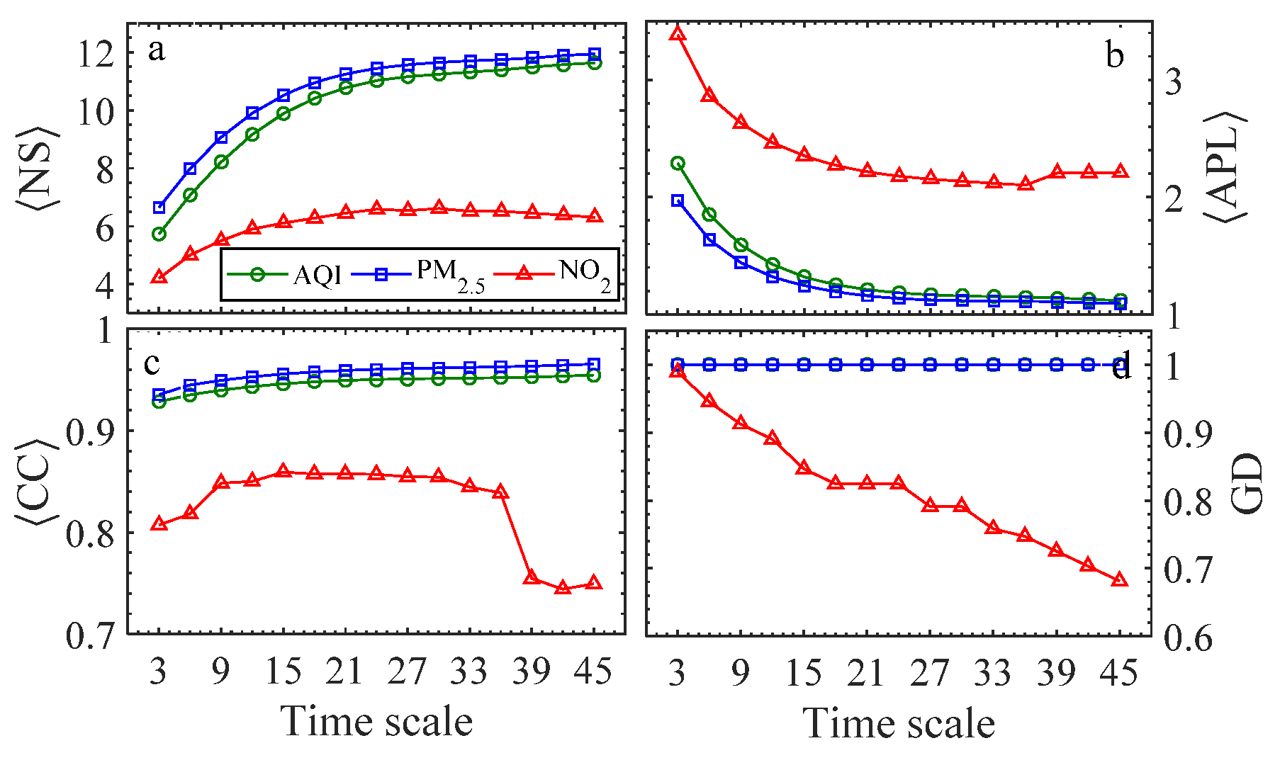
Finally, let us focus on the global network properties of the three air environment factors with respect to the different time scales, as shown in Figure 5. The figures of average network properties of node strength, average path length, clustering coefficient as well as graph density show again that the AQI is closer to PM_2.5 than NO₂ at every given time scale. It confirms again that the AQI mainly depends on PM_2.5. The dynamical change process of the four network attributes with the various time scales allows us to easily access the network structure. Specifically, the average node strength ($〈NS〉$) of AQI and PM_2.5 is increased with lengthening time scales, while the $〈NS〉$ of NO₂ tends to be stable after 21 days. The rate of change for both AQI and PM_2.5 is larger than that of NO₂, suggesting that the co-movement of PM_2.5 is more significant among the 14 cities with increasing time scales. This finding is supported by the decreasing global average path length ($〈APL〉$), as shown in Figure 5b, which explains that PM_2.5 is easy to diffuse among different cities as time goes on while the NO₂ transmission is much more difficult. The average clustering coefficient ($〈CC〉$) also confirms this conclusion. The stable value of $〈CC〉$ for both AQI and PM_2.5 with the different time scales shows that the high regional co-movement of the PM_2.5 continued from a short period to a long period in Hunan Province. In contrast, the $〈CC〉$ of NO₂ fell off after about 36 days, implying that the aggregation effect of NO₂ among the 14 cities is significantly weakened after approximately one month. It shows that the correlation of NO₂ among the 14 cities does not last over the long term. In the end, the fact that the graph density of both AQI and PM_2.5 is always 1 means the two networks are always fully connected, while the graph density of NO₂’s network decreases with the increasing time scales. This is because the correlated significance of the NO₂ between every pair of cities gradually weakens with the lengthening of time scale, which causes some nodes to be disconnected. The above results confirm that the co-movement of the PM2.5 pollutants among the 14 cities is significantly stronger than NO₂ pollutants. The co-movement of the PM2.5 pollutant can last 45 days while that of the NO₂ pollutant decreases over time. By analyzing correlations of the topological properties at the given scales (see Figure 6—the darker the color is, the stronger the negative correlation is, with the positive correlation increasing with lighter colors), it can be found that: the $〈NS〉$ shows a strong positive correlation with $〈CC〉$ and strong negative correlation with $〈APL〉$ for the AQI and PM_2.5. However, the abnormal trend of $〈CC〉$ for NO₂ destroys the correlation between it and the other two properties of NO₂. In addition, except $〈CC〉$ of NO₂, the other properties show a positive correlation with the identical properties between the different environmental factors.

3.4. Clustering Analysis

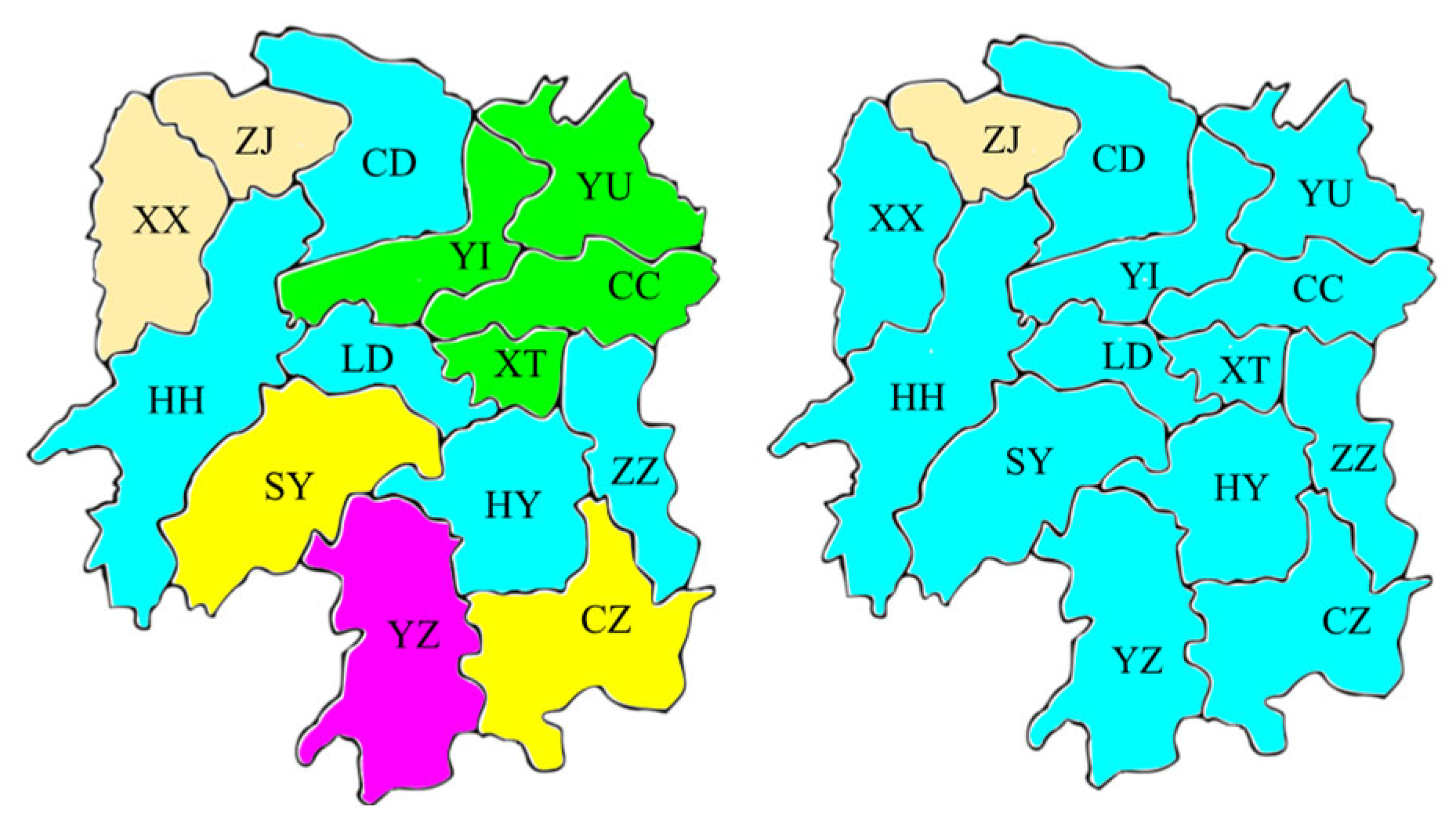
In this subsection, we focus on the clustering of the two pollutants for the 14 cities in Hunan Province to provide a theoretical basis for regional joint air pollution control. To do so, we utilize the spectral clustering algorithm introduced in Section 2.4. The critical problem of clustering is to determine the number of classes (K). Here, we employ two indicators, i.e., Davies-Bouldin and silhouette coefficient to fulfill this task. As seen in Figure 7, the two indicators show the consistent optimal K for each pollutant index, namely, K = 5 for PM_2.5 and K = 2 for NO₂. Therefore, we wish to cluster the 14 cities into 5 regions and 2 regions for the co-governance of PM_2.5 and NO₂, respectively. As shown in Figure 8, for PM_2.5, the clustering basically conforms to geographical proximity, indicating that the factor of geographical proximity is still the primary consideration for the co-governance of PM_2.5. Accordingly, the cities in the same region should establish a mechanism of regional joint prevention and control coordination, regional information sharing, unified emergency response, and joint law enforcement for limiting automobile exhaust emissions, industrial dust, dust smog, etc. For NO₂, the 13 cities are clustered together except for Zhangjiajie city (ZJ). Zhangjiajie city is a tourist city with large forest coverage, where less fossil fuel combustion takes place. For the 13 cities, the provincial government should implement unified deployment to shut down the ill-formed chemical plants and small-scale but highly-polluting mining processing activities, and limit emissions from thermal power plants.

4. Discussion and Conclusions

In this work, we initiated a study on the air quality of 14 cities in Hunan Province from a multiscale statistical perspective. It mainly focused on the impact of fine particulate matter (PM_2.5) and nitrogen compounds (NO₂) on air quality (AQI) at different time scales. In addition, a regional cooperation joint pollution control program was provided according to the clustering analysis for the two pollutants of 14 cities. To this end, several physical statistical methods were employed to study the above issues. We utilized the HXA method to calculate a family of cross-correlation coefficients at different time scales for the 91 pairs of cities. Additionally, a significant test was used to determine the correlation’s significance, which is the base of the establishment of the network edge connection. Accordingly, the air pollutant networks were constructed at different time scales among the 14 cities. Four common network properties of node strength, clustering coefficient, average path length, and graph density were then used to analyze the network structures of different time scales. J-S divergence was used to assess the difference between those network properties. Three main findings can be concluded. Firstly, the correlation of the pollutants’ concentration among the 14 cities in 15 days can best reflect the air quality of Hunan Province. Compared with NO₂, PM_2.5 influences the air quality of Hunan Province more on each time scale. Secondly, NO₂ affects the air quality of the 14 cities more in short-time intervals than in long-time intervals. In contrast, PM_2.5 dominated in AQI of Hunan Province in both short and long-time intervals. Moreover, the aggregation effect of NO₂ prevails in short and median time scales, while that of PM_2.5 is more serious. Thirdly, the co-movement of the PM_2.5 pollutants among the 14 cities is significantly stronger than that of the NO₂ pollutants. The co-movement of the PM_2.5 pollutants can last at least 45 days, while that of NO₂ pollutants will gradually decline as time goes on. Furthermore, in considering the mobility of air pollution, which will affect the air quality of surrounding areas, according to the node strength attribute, we utilized the spectral clustering algorithm to cluster the 14 cities into five regions and two regions for jointly governing the PM_2.5 pollutant and NO₂ pollutant, respectively. For the co-governance of PM_2.5 pollutants, the classification of five regions basically conforms to geographical proximity, indicating that the factor of geographical proximity is still the primary consideration for the co-governance of PM_2.5. However, for the NO₂, the 13 cities are clustered together, except Zhangjiajie city (ZJ). According to our statistical analysis of the air pollutants in Hunan Province, our suggestions are, on one hand, to strengthen the governance for the internal pollution sources of a city and develop air pollution prevention strategies for the city according to its specific pollutants, and on the other, uniting the regions to coordinate resources and carry out regional joint control in an orderly, step-by-step way.

Finally, we highlight that this work is conducted based on the statistical perspective. Most existing studies on air pollution in Hunan Province are from the perspective of the formation and diffusion mechanism of pollutants. This work is based on data-driven processes, which is an important supplement to the existing research mechanisms. We emphasize again that none of the methods employed is unique for our studied purpose, but they are common methods and easy to implement. The findings can provide a reference for environmental scientists or environmental protection departments. Given the powerful information mining function of complex networks, in our forthcoming work we would like to investigate the spread of pollutants in the existing networks of 14 cities of Hunan Province and further trace the source of the pollutants by using the network node attributes, such as shortest propagation paths or transfer rates and attraction rates. Another interesting area of research to consider is the interaction between different pollutants by using multiple networks technology [43].

References

1. Wang, F.; Wang, L.; Chen, Y. A DFA-based bivariate regression model for estimating the dependence of PM2.5 among neighbouring cities. Sci. Rep. 2018, 8, 7475. [Google Scholar] [CrossRef] [PubMed] [Green Version]
2. Wang, S.; Hao, J. Air quality management in China: Issues, challenges, and options. J. Environ. Sci. 2012, 24, 2–13. [Google Scholar] [CrossRef] [PubMed]
3. Han, L.J.; Zhou, W.Q.; Li, W.F. Increasing impact of urban fine particles (pm 2.5) on areas surrounding Chinese cities. Sci. Rep. 2015, 5, 12467. [Google Scholar] [CrossRef] [PubMed] [Green Version]
4. Gousseau, P.; Blocken, B.; van Heijst, G. Large-Eddy Simulation of pollutant dispersion around a cubical building: Analysis of the turbulent mass transport mechanism by unsteady concentration and velocity statistics. Environ. Pollut. 2012, 167, 47–57. [Google Scholar] [CrossRef] [PubMed]
5. Shi, K. Detrended cross-correlation analysis of temperature, rainfall, pm10 and ambient dioxins in Hong Kong. Atmos. Environ. 2014, 97, 130–135. [Google Scholar] [CrossRef]
6. Liu, Y.; Zhou, Y.; Lu, J. Exploring the relationship between air pollution and meteorological conditions in China under environmental governance. Sci. Rep. 2020, 10, 1–11. [Google Scholar] [CrossRef]
7. Wang, F.; Fan, Q. Coupling correlation detrended analysis for multiple nonstationary series. Commun. Nonlinear Sci. Numer. Simul. 2021, 94, 105579. [Google Scholar] [CrossRef]
8. Long, W.; Zhou, Y.; Liu, P. Numerical simulation of the influence of major meteorological elements on the concentration of air pollutants during rainfall over Sichuan Basin of China. Atmos. Pollut. Res. 2020, 11, 2036–2048. [Google Scholar] [CrossRef]
9. Zebende, G.F.; da Silva Filho, A.M. Detrended multiple cross-correlation coefficient. Physica A 2018, 510, 91–97. [Google Scholar] [CrossRef]
10. Wang, F.; Xu, J.; Fan, Q. Statistical properties of the detrended multiple cross-correlation coefficient. Commun. Nonlinear Sci. Numer. Simul. 2021, 99, 105781. [Google Scholar] [CrossRef]
11. Wang, F.; Wang, L.; Chen, Y. Detecting PM2.5’s correlations between neighboring cities using a time-lagged cross-correlation coefficient. Sci. Rep. 2017, 7, 10109. [Google Scholar] [CrossRef] [Green Version]
12. Chen, Z.; Xu, B.; Cai, J.; Gao, B. Understanding temporal patterns and characteristics of air quality in Beijing: A local and regional perspective. Atmos. Environ. 2016, 127, 303–315. [Google Scholar] [CrossRef]
13. Liu, X.; Schnelle-Kreis, J.; Zhang, X.; Bendl, J.; Khedr, M.; Jakobi, G.; Schloter-Hai, B.; Hovorka, J.; Zimmermann, R. Integration of air pollution data collected by mobile measurement to derive a preliminary spatiotemporal air pollution profile from two neighboring German-Czech border villages. Sci. Total Environ. 2020, 722, 137632. [Google Scholar] [CrossRef]
14. Chen, G.R.; Wang, X.F.; Li, X. Introduction to Complex Networks: Models, Structures and Dynamics; Higher Education Press: Beijing, China, 2015. [Google Scholar]
15. Yang, Y.; Yang, H. Complex network-based time series analysis. Physica A 2008, 387, 1381–1386. [Google Scholar] [CrossRef]
16. Donner, R.V.; Zou, Y.; Donges, J.; Marwan, N.; Kurths, J. Recurrence networks—A novel paradigm for nonlinear time series analysis. New J. Phys. 2010, 12, 033025. [Google Scholar] [CrossRef] [Green Version]
17. Xu, X.; Zhang, J.; Small, M. Superfamily phenomena and motifs of networks induced from time series. Proc. Natl. Acad. Sci. USA 2008, 105, 19601–19605. [Google Scholar] [CrossRef] [Green Version]
18. Lacasa, L.; Luque, B.; Ballesteros, F.; Luque, J.; Nuño, J.C. From time series to complex networks: The visibility graph. Proc. Natl. Acad. Sci. USA 2008, 105, 4972–4975. [Google Scholar] [CrossRef] [Green Version]
19. Luque, B.; Lacasa, L.; Ballesteros, F.; Luque, J. Horizontal visibility graphs: Exact results for random time series. Phys. Rev. E 2009, 80, 046103. [Google Scholar] [CrossRef] [Green Version]
20. Nicolis, G.; Cantú, G.A.; Nicolis, C. Dynamical aspects of interaction networks. Int. J. Bifurc. Chaos 2005, 15, 3467–3480. [Google Scholar] [CrossRef]
21. Donner, R.; Small, M.; Donges, J.; Marwan, N.; Zou, Y.; Xiang, R.; Kurths, J. Recurrence-based time series analysis by means of complex network methods. Int. J. Bifurc. Chaos 2011, 21, 1019–1046. [Google Scholar] [CrossRef]
22. Zou, Y.; Donner, R.V.; Marwan, N.; Donges, J.F.; Kurths, J. Complex network approaches to nonlinear time series analysis. Phys. Rep. 2019, 787, 1–97. [Google Scholar] [CrossRef]
23. Song, C.; Huang, G.; Zhang, B.; Yin, B.; Lu, H. Modeling air pollution transmission behavior as complex network and mining key monitoring station. IEEE Access 2019, 7, 121245–121254. [Google Scholar] [CrossRef]
24. Plocoste, T.; Carmona-Cabezas, R.; de Ravé, E.G.; Jiménez-Hornero, F.J. Wet scavenging process of particulate matter (PM10): A multivariate complex network approach. Atmos. Pollut. Res. 2021, 12, 101095. [Google Scholar] [CrossRef]
25. Zhang, Z.; Wang, F.; Shen, L.; Xie, Q. Multiscale time-lagged correlation networks for detecting air pollution interaction. Physica A 2022, 602, 127627. [Google Scholar] [CrossRef]
26. Dai, Y.H.; Zhou, W.X. Temporal and spatial correlation patterns of air pollutants in Chinese cities. PLoS ONE 2017, 12, e0182724. [Google Scholar] [CrossRef] [PubMed] [Green Version]
27. Chang, F.; Ge, L.; Li, S.; Wu, K.; Wang, Y. Self-adaptive spatial–temporal network based on heterogeneous data for air quality prediction. Connect. Sci. 2021, 33, 427–446. [Google Scholar] [CrossRef]
28. Bulletin of the Second National Pollution Source Census in Hunan Province. Available online: http://www.hunan.gov.cn/xxgk/tzgg/szbm/202012/t20201228_14086835.html (accessed on 10 November 2022).
29. Kristoufek, L. Multifractal height cross-correlation analysis: A new method for analyzing long-range cross-correlations. Europhys. Lett. 2011, 95, 68001. [Google Scholar] [CrossRef] [Green Version]
30. Wang, F.; Yang, Z.; Wang, L. Detecting and quantifying cross-correlations by analogous multifractal height cross-correlation analysis. Physica A 2016, 444, 954–962. [Google Scholar] [CrossRef]
31. Wang, F.; Wang, L.; Chen, Y. Quantifying the range of cross-correlated fluctuations using a q–L dependent AHXA coefficient. Physica A 2018, 494, 454–464. [Google Scholar] [CrossRef]
32. Barabási, A.L.; Vicsek, T. Multifractality of self-affine fractals. Phys. Rev. A 1991, 44, 2730. [Google Scholar] [CrossRef]
33. Podobnik, B.; Stanley, H.E. Detrended cross-correlation analysis: A new method for analyzing two nonstationary time series. Phys. Rev. Lett. 2008, 100, 084102. [Google Scholar] [CrossRef] [Green Version]
34. Podobnik, B.; Jiang, Z.-Q.; Zhou, W.-X.; Stanley, H. Statistical tests for power-law cross-correlated processes. Phys. Rev. E 2011, 84, 066118. [Google Scholar] [CrossRef] [Green Version]
35. Barrat, A.; Barthelemy, M.; Pastor-Satorras, R.; Vespignani, A. The architecture of complex weighted networks. Proc. Natl. Acad. Sci. USA 2004, 101, 3747–3752. [Google Scholar] [CrossRef] [Green Version]
36. Holme, P.; Park, S.M.; Kim, B.J.; Edling, C.R. Korean university life in a network perspective: Dynamics of a large affiliation network. Physica A 2007, 373, 821–830. [Google Scholar] [CrossRef] [Green Version]
37. Opsahl, T.; Panzarasa, P. Clustering in weighted networks. Soc. Netw. 2009, 31, 155–163. [Google Scholar] [CrossRef]
38. Mhatre, V.; Rosenberg, C. Homogeneous vs heterogeneous clustered sensor networks: A comparative study. In Proceedings of the 2004 IEEE International Conference on Communications (IEEE Cat. No. 04CH37577), Paris, France, 20–24 June 2004; Volume 6, pp. 3646–3651. [Google Scholar]
39. Hougardy, S. The Floyd–Warshall algorithm on graphs with negative cycles. Inf. Process. Lett. 2010, 110, 279–281. [Google Scholar] [CrossRef]
40. Nielsen, F. On the Jensen–Shannon symmetrization of distances relying on abstract means. Entropy 2019, 21, 485. [Google Scholar] [CrossRef] [Green Version]
41. Von Luxburg, U. A tutorial on spectral clustering. Stat. Comput. 2007, 17, 395–416. [Google Scholar] [CrossRef]
42. Wang, F.; Zhao, W.; Jiang, S. Detecting asynchrony of two series using multiscale cross-trend sample entropy. Nonlinear Dyn. 2020, 99, 1451–1465. [Google Scholar] [CrossRef]
43. Menichetti, G.; Remondini, D.; Panzarasa, P.; Mondragón, R.J.; Bianconi, G. Weighted Multiplex Networks. PLoS ONE 2014, 9, e97857. [Google Scholar] [CrossRef]
Figure 1. HXA-based cross-correlation coefficient of the AQI (a) and the two pollutants (b,c) between every pair of cities with respect to time scale. The black dotted line denotes the critical value under 0.05 significant level. The area above this line means correlation significance.
Atmosphere 14 00055 g001
Figure 2. The left panel is the PDF of scale-dependent edge weights for three indexes of AQI, PM2.5, and NO2 at three given time scales, namely, small scale (a, d, g), median scale (b, e, h) and large scale (c, f, i). There is a similar shape of the PDF between the AQI and PM2.5, while a significant difference can be observed between them and that of NO2. The right panel is the J-S divergence of the edge weight of AQI’s network and that of the two pollutants’ networks with respect to different time scales.
Atmosphere 14 00055 g002
Figure 3. Networks graph of NO2 at (a) small time scale, (b) medium time scale, and (c) large time scale.
Atmosphere 14 00055 g003
Figure 4. PDF of node strength (the first column), clustering coefficient (the second column), and average path length (the third column) for three indexes of AQI (the first row), PM2.5 (the second row) and NO2 (the third row). There is a similar shape of the PDF between the AQI and PM2.5, while a significant difference can be observed between them and that of NO2. The right panel shows the J-S divergence of the PDF of the clustering coefficient, node strength, and average path length of the AQI series and the two pollutants’ series for the 14 cities at different time scales.
Atmosphere 14 00055 g004
Figure 5. The four networks’ properties to different time scales for the AQI, PM2.5, and NO2 series. (ad) is <NS>, <APL>, <CC>, and GD, respectively.
Atmosphere 14 00055 g005
Figure 6. Diagram for the correlation matrix of topological parameters. The subscripts 1, 2, and 3 of the three parameters represent AQI, PM2.5, and NO2, respectively.
Atmosphere 14 00055 g006
Figure 7. Evaluation of spectral clustering algorithm of PM2.5 and NO2 with respect to the value of K. Two criteria are used, namely, the Davies-Bouldin index (DB) and silhouette coefficient (SC). The criterion values in the green rectangle refer to the optimal K.
Atmosphere 14 00055 g007
Figure 8. Clustering of the PM2.5 (left panel) and NO2 (right panel) of 14 cities in Hunan Province.
Atmosphere 14 00055 g008