
Precipitation Extremes and Their Synoptic Models in the Northwest European Sector of the Arctic during the Cold Season


Abstract
1. Introduction
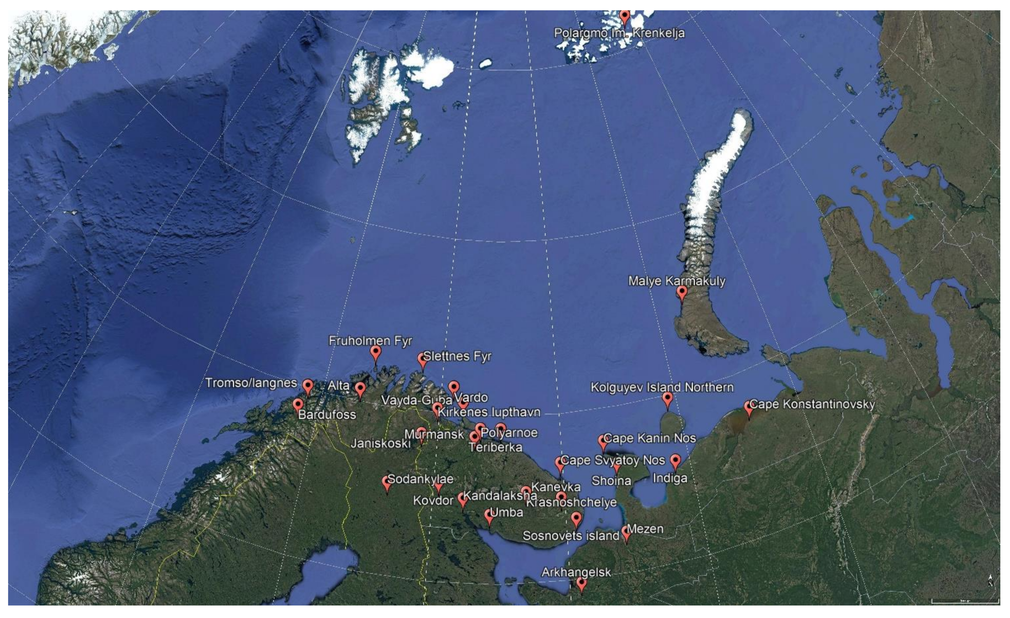
2. Data
3. Methodology
4. Results and Discussions
4.1. Statistical Features of the Observed Daily Precipitation Sums
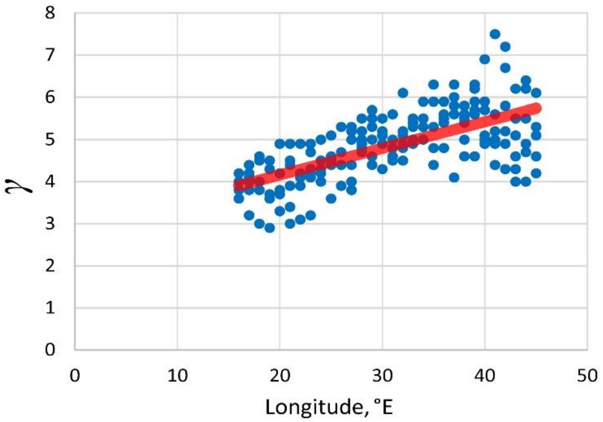
4.2. The Pareto Distributions in Data of the ERA5
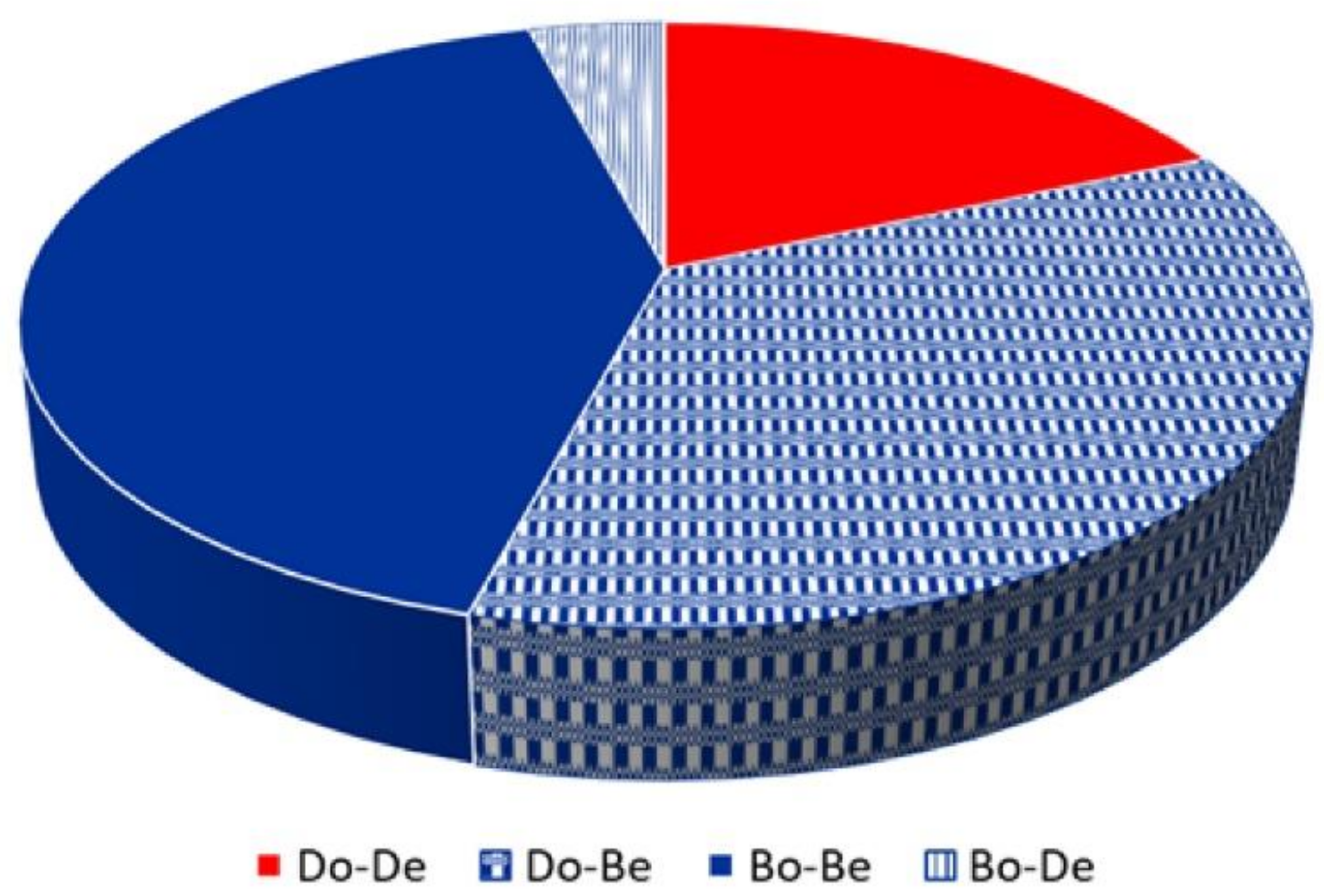
4.3. Precipitation Extrema and Extratropical Cyclones
4.4. Precipitation Extrema and Role of the Polar Lows
5. Conclusions
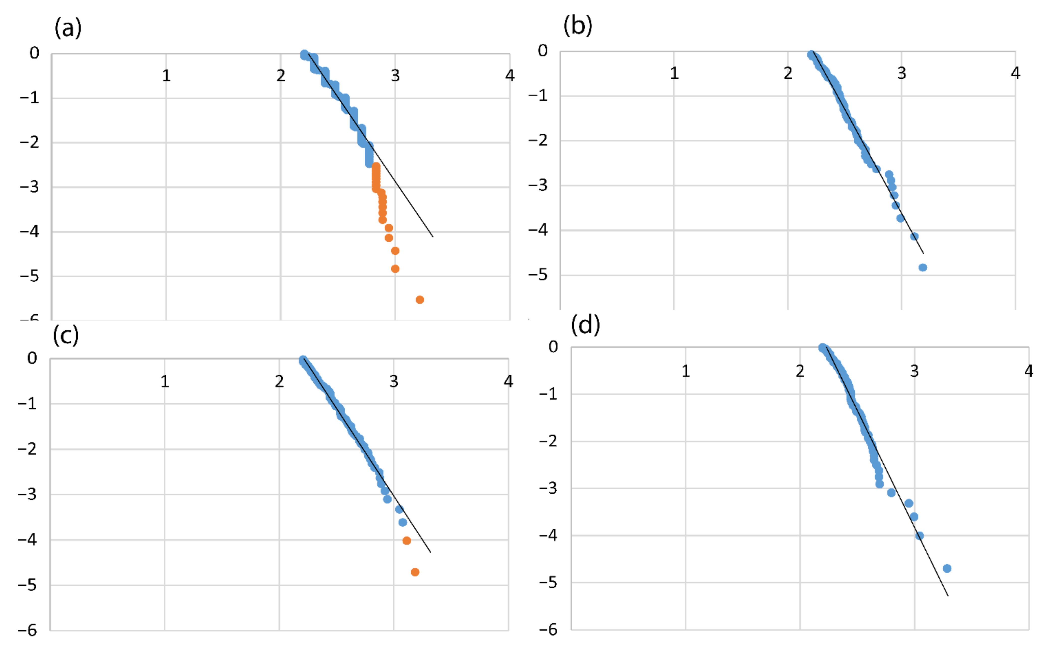
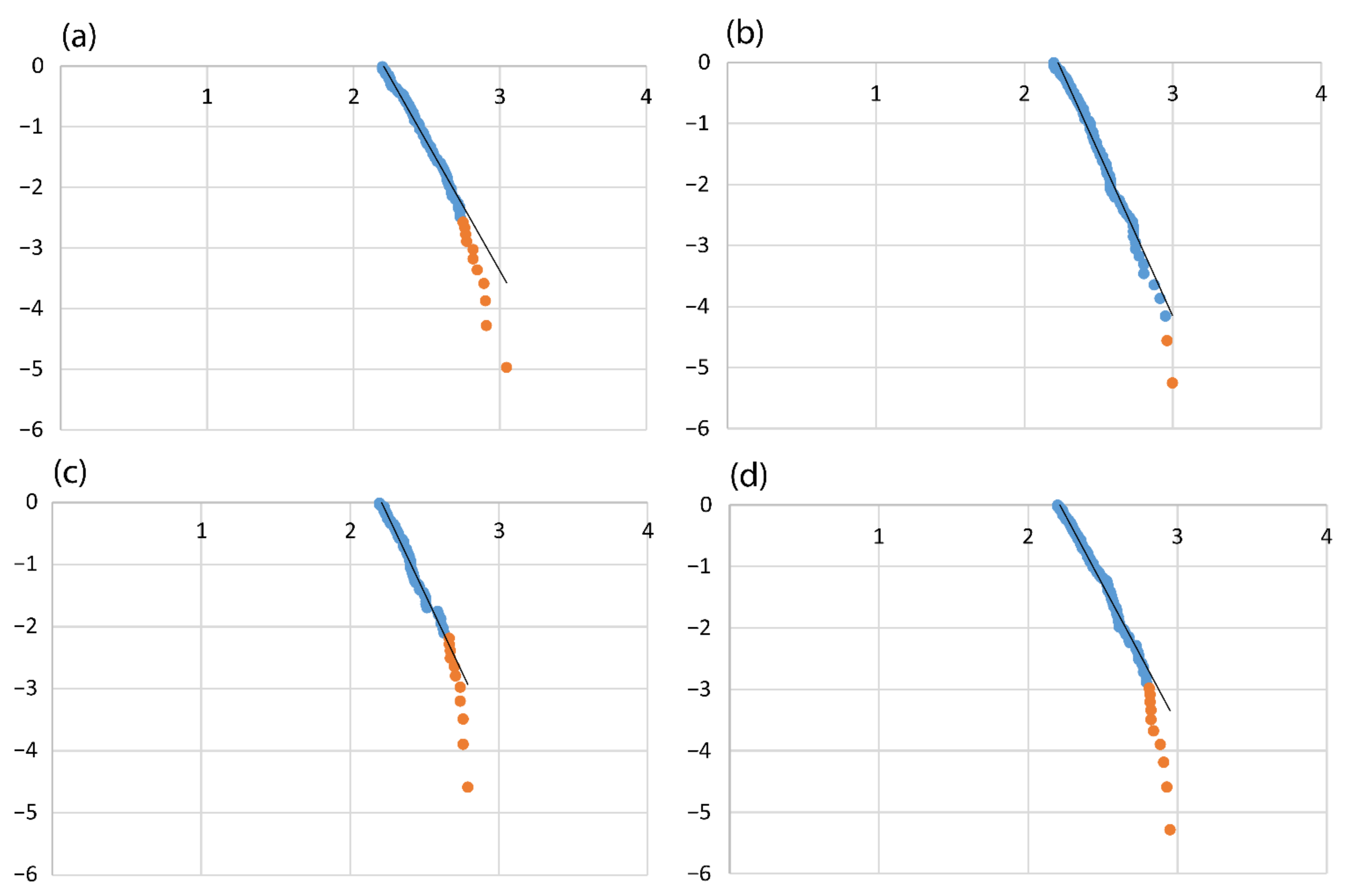
- It was demonstrated that the Pareto distributions are close for the extremes that were extracted from both the re-analysis data and observational data. However, the strongest episodes did not fall into this distribution. For them, the correspondence between the absolute value of the anomaly and its probability is completely lost, thereby signifying that any anomaly can occur. This means that super-large anomalies do not obey the statistical law common to all other extremes. It is no wonder, according to this sign, they are labelled as dragons. However, the statement “any anomalies” does not mean that the extremes can be arbitrarily large. They do not exceed the marginal values that are typical for this type of climate and season. This effect appears to be one of saturation when the limit is approached.
- Let us focus on the widely used practice of utilizing quantile values (k = 0.95 or 0.99) for the analysis of precipitation anomalies. Clearly, this procedure is correct if the CDF is adequate for the entire domain and if the distribution of events exceeding the selected quantile value is given by the expression 1-W(pk). However, in the cases discussed in this article, this leads to distortions, as the structure of the “tip of the tail” of the distribution is completely different from that of the regular base function. The procedure of “pulling” the base Pareto law into the region of “superlarge” precipitation significantly underestimates the return periods of the observed precipitation extrema. This circumstance requires careful use of quantile analysis. For this, it is necessary to consider the situation in which the samples belong to different distribution functions.
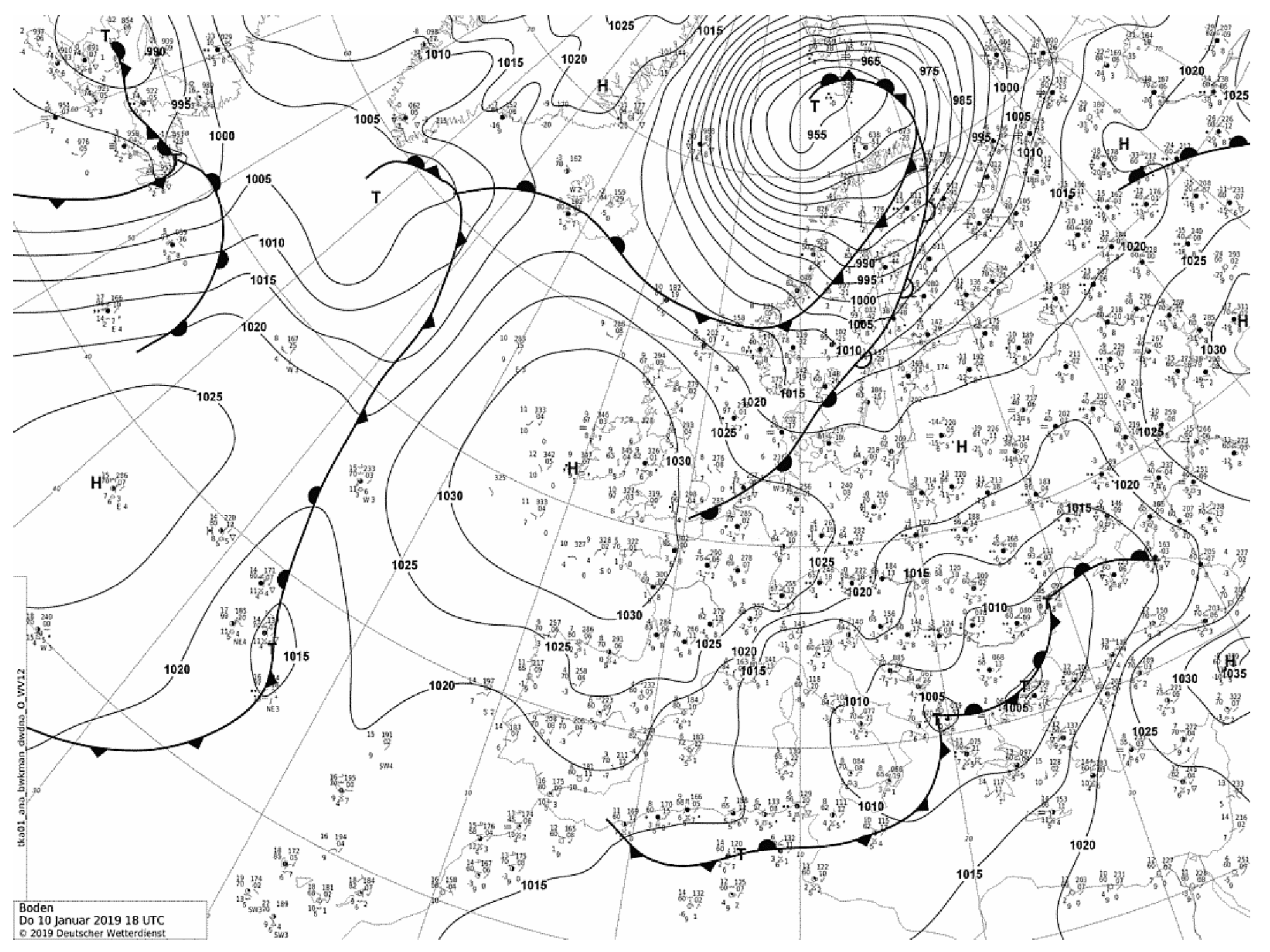
- Extreme precipitation in the Barents region of the Arctic during the cold period was caused by the advection of moist air masses from the Atlantic Ocean. The transfer occurs in the circulation system of the intense polar front cyclones. Sometimes mesoscale convective systems are embedded in atmospheric fronts, thereby making a significant contribution to the formation of precipitation. The influence of polar lows on the formation of large amounts of precipitation was practically non-existent.
- Intensive cyclones penetrate the Arctic more often during climate warming. In winter, this happens due to the modification of the regional circulation, the increase in meridional processes during blocking [28], and due to the increase in the open water zone (due to the reduction in the area of sea ice), in which it is easier for cyclones to move. Cyclones work as a positive feedback factor. This should lead to a transformation of typical CDF, as modern “chaotic” dragons will become “regular” black swans. This change in the statistics of extreme events reflects the nonstationarity of the climate state.
Author Contributions
Funding
Data Availability Statement
Conflicts of Interest
References
- Serreze, M.C.; Barry, R.G. Processes and Impacts of Arctic Amplification: A Research Synthesis. Glob. Planet. Chang. 2011, 77, 85–96. [Google Scholar] [CrossRef]
- Polyakov, I.V.; Pnyushkov, A.V.; Alkire, M.B.; Ashik, I.M.; Baumann, T.M.; Carmack, E.C.; Goszczko, I.; Guthrie, J.; Ivanov, V.V.; Kanzow, T.; et al. Greater role for Atlantic inflows on sea-ice loss in the Eurasian Basin of the Arctic Ocean. Science 2017, 356, 285–291. [Google Scholar] [CrossRef] [PubMed]
- Cohen, J.; Screen, J.A.; Furtado, J.C.; Barlow, M.; Whittleston, D.; Coumou, D.; Francis, J.; Dethloff, K.; Entekhabi, D.; Overland, J.; et al. Recent Arctic Amplification and Extreme Mid-Latitude Weather. Nat. Geosci. 2014, 7, 627–637. [Google Scholar] [CrossRef]
- Ye, K.; Wu, R.; Liu, Y. Interdecadal Changes of Eurasian Snow, Surface Temperature and Atmospheric Circulation in the Late 1980s. J. Geophys. Res. Atmos. 2015, 120, 2738–2753. [Google Scholar] [CrossRef]
- Kislov, A.; Antipina, U.I.; Korneva, I.A. Precipitation extrema over the European sector of the Arctic during the summer time: Statistics and synoptic models. Russ. Meteorol. Hydrol. 2012, 46, 434–443. [Google Scholar] [CrossRef]
- Zolina, O.; Kapala, A.; Simmer, C.; Gulev, S.K. Analysis of extreme precipitation over Europe from different reanalyses: A comparative assessment. Glob. Planet. Chang. 2004, 44, 129–161. [Google Scholar] [CrossRef]
- Ben Alaya, M.A.; Zwiers, F.W.; Zhang, X. A bivariate approach to estimating the probability of very extreme precipitation events. Weather Clim. Extrem. 2020, 30, 100290. [Google Scholar] [CrossRef]
- Katz, R.W. Extreme value theory for precipitation: Sensitivity analysis for climate change. Adv. Water Resour. 1999, 23, 133–139. [Google Scholar] [CrossRef]
- Kharin, V.V.; Zwiers, F.W.; Zhang, X.B.; Hegerl, G.C. Changes in temperature and precipitation extremes in the IPCC ensemble of global coupled model simulations. J. Clim. 2007, 20, 1419–1444. [Google Scholar] [CrossRef]
- Semenov, V.A.; Bengtsson, L. Secular trends in daily precipitation characteristics: Greenhouse gas simulation with a coupled AOGCM. Clim. Dyn. 2002, 19, 123–140. [Google Scholar] [CrossRef]
- Maraun, D.; Wetterhall, F.; Ireson, A.M.; Chandler, R.E. Precipitation downscaling under climate change. Recent developments to bridge the gap between dynamical models and the end user. Rev. Geophys. 2010, 48, RG3003. [Google Scholar] [CrossRef]
- Beirlant, J.; Goegebeur, Y.; Segers, J.; Teugels, J.; De Waal, D.; Ferro, C. Statistics of Extremes: Theory and Applications; Willey Series in Probability and Statistics; John Wiley & Sons Ltd.: Chichester, UK, 2004. [Google Scholar] [CrossRef]
- Coles, S. An Introduction to Statistical Modeling of Extreme Values; Springer Series in Statistics; Springer: Berlin/Heidelberg, Germany, 2001. [Google Scholar]
- Coles, S.; Walshaw, D. Directional Modelling of Extreme Wind Speeds. J. R. Stat. Soc. Ser. C (Appl. Stat.) 1994, 43, 139–157. [Google Scholar] [CrossRef]
- Kislov, A.; Matveeva, T. An Extreme Value Analysis of Wind Speed over the European and Siberian Parts of Arctic Region. Atmos. Clim. Sci. 2016, 6, 205–223. [Google Scholar] [CrossRef][Green Version]
- Myslenkov, S.; Platonov, V.; Kislov, A.; Silvestrova, K.; Medvedev, I. Wave climate and storm activity in the Kara sea. Thirty-Nine-Year Wave Hindcast, Storm Activity, and Probability Analysis of Storm Waves in the Kara Sea, Russia. Water 2021, 13, 648. [Google Scholar] [CrossRef]
- Taleb, N.N. The Black Swan: The Impact of the Highly Improbable, 2nd ed.; Penguin: New York, NY, USA, 2010. [Google Scholar]
- Sornette, D. Dragon-Kings, Black Swans and the Prediction of Crises. Int. J. Terraspace Sci. Eng. 2009, 2, 1–18. [Google Scholar] [CrossRef]
- Kislov, A.; Matveeva, T. The Monsoon over the Barents Sea and Kara Sea. Atmos. Clim. Sci. 2020, 10, 339–356. [Google Scholar] [CrossRef]
- Rasmussen, E.A.; Turner, J. Polar Lows: Mesoscale Weather Systems in the Polar Regions; Cambridge University Press: Cambridge, UK, 2003. [Google Scholar]
- Hersbach, H.; Dee, D. ERA-5 Reanalysis Is in Production. ECMWF Newsl. 2016, 147, 5–6. [Google Scholar]
- Hersbach, H.; Bell, B.; Berrisford, P.; Horanyi, A.; Sabater, J.M.; Nicolas, J.; Radu, R.; Schepers, D.; Simmons, A.; Soci, C.; et al. Global Reanalysis: Goodbye ERAInterim, Hello ERA5. ECMWF Newsl. 2019, 159, 17–24. [Google Scholar]
- Rojo, M.; Claud, C.; Noer, G.; Carleton, A. In situ measurements of surface winds, waves, and sea state in polar lows over the North Atlantic. J. Geophys. Res. Atmos. 2019, 124, 700–718. [Google Scholar] [CrossRef]
- Smirnova, J.E.; Golubkin, P.A.; Bobylev, L.P.; Zabolotskikh, E.V.; Chapron, B. Polar low climatology over the Nordic and Barents seas based on satellite passive microwave data. Geophys. Res. Lett. 2015, 42, 5603–5609. [Google Scholar] [CrossRef]
- Revokatova, A.; Nikitin, M.; Rivin, G.; Rozinkina, I.; Nikitin, A.; Tatarinovich, E. High-Resolution Simulation of Polar Lows over Norwegian and Barents Seas Using the COSMO-CLM and ICON Models for the 2019–2020 Cold Season. Atmosphere 2021, 12, 137. [Google Scholar] [CrossRef]
- Golubkin, P.; Smirnova, J.; Bobylev, L. Satellite-Derived Spatio-Temporal Distribution and Parameters of North Atlantic Polar Lows for 2015–2017. Atmosphere 2021, 12, 224. [Google Scholar] [CrossRef]
- Sornette, D.; Ouillon, G. Dragon-Kings: Mechanisms, Statistical Methods and Empirical Evidence. Eur. Phys. J. Spec. Top. 2012, 205, 1–26. [Google Scholar] [CrossRef]
- Kislov, A.; Sokolikhina, N.; Semenov, E.; Tudriy, K. Blocking Anticyclone in the Atlantic Sector of the Arctic as an Example of an Individual Atmospheric Vortex. Atmos. Clim. Sci. 2017, 7, 323–336. [Google Scholar] [CrossRef]


| Name of Observation Stations | γ |
|---|---|
| Bardufoss | 4.0 |
| Tromso/langnes | 3.0 |
| Tromsoe | 3.2 |
| Alta | 6.8 |
| Fruholmen Fyr | 3.8 |
| Kirkenes lufthavn | 5.2 |
| Sodankylae | 7.0 |
| Vayda-Guba | 3.8 |
| Polyarnoe | 3.9 |
| Umba | 3.7 |
| Cape Kanin Nos | 4.2 |
| Cape Svyatoy Nos | 4.0 |
| Kandalaksha | 4.7 |
| Kanevka | 4.8 |
| Cape Konstantinovsky | 2.9 |
| Indiga | 4.6 |
| Kovdor | 3.5 |
| Kolguyev Island Northern | 5.8 |
| Krasnoshchelye | 3.8 |
| Mezen | 4.2 |
| Arkhangelsk | 5.0 |
| Teriberka | 3.9 |
| Vardo | 5.4 |
| Murmansk | 4.6 |
| Shoina | 3.8 |
| Sosnovets island | 3.8 |
| Janiskoski | 4.0 |
| Slettnes Fyr | 3.8 |
| Mean | 4.4 |
| Mean ± Std | 3.4–5.4 |
| Data | Maximum of Precipitation, mm | Region of Appearances | Precipitable Water *, kg·m−2 | Rank |
|---|---|---|---|---|
| 10 January 2019 | 28 | 75 N 16–28 E | 5 | 1–3 |
| 18 | 74 N 16–29 E | <10 | ||
| 18 | 73 N 19–24 E | <10 | ||
| 20 | 72 N 16–27 E | <10 | ||
| 18 | 71 N 20–21 E | <20 | ||
| 15 | 70 N 16–17 E | <20 | ||
| 6 January 2009 – 7 January 2009 | 30 | 73 N 26–35 E | 4 | 30 |
| 30 November 2019 | 27 | 75 N 17–37 E | 7 | 1–3 |
| 29 | 74 N 26–42 E | 1–3 | ||
| 19 | 73 N 37–41 E | <10 | ||
| 15 | 72 N 16–27 E | <20 | ||
| 19 January 2000 | 16 | 74 N 40–42 E | 3 | <10 |
| 14 | 73 N 37–39 E | <10 |
Publisher’s Note: MDPI stays neutral with regard to jurisdictional claims in published maps and institutional affiliations. |
© 2022 by the authors. Licensee MDPI, Basel, Switzerland. This article is an open access article distributed under the terms and conditions of the Creative Commons Attribution (CC BY) license (https://creativecommons.org/licenses/by/4.0/).
Share and Cite
Kislov, A.; Matveeva, T.; Antipina, U. Precipitation Extremes and Their Synoptic Models in the Northwest European Sector of the Arctic during the Cold Season. Atmosphere 2022, 13, 1116. https://doi.org/10.3390/atmos13071116
Kislov A, Matveeva T, Antipina U. Precipitation Extremes and Their Synoptic Models in the Northwest European Sector of the Arctic during the Cold Season. Atmosphere. 2022; 13(7):1116. https://doi.org/10.3390/atmos13071116
Chicago/Turabian StyleKislov, Alexander, Tatiana Matveeva, and Uliana Antipina. 2022. "Precipitation Extremes and Their Synoptic Models in the Northwest European Sector of the Arctic during the Cold Season" Atmosphere 13, no. 7: 1116. https://doi.org/10.3390/atmos13071116
APA StyleKislov, A., Matveeva, T., & Antipina, U. (2022). Precipitation Extremes and Their Synoptic Models in the Northwest European Sector of the Arctic during the Cold Season. Atmosphere, 13(7), 1116. https://doi.org/10.3390/atmos13071116