Abstract
In present China, continuing to control PM2.5 (particulate matter < 2.5 μm) and preventing the rise of O3 are the most urgent environmental tasks in its air clean actions. Considering that NO2 is an important precursor of PM2.5 and O3, a comprehensive analysis around this pollutant was conducted based on the real-time-monitoring data from Jan 2018 to Mar 2019 in 11 prefecture-level cities in Shanxi Province of China. The results showed that the annual average concentration of NO2 in Shanxi prefecture-level cities is mainly distributed in the range of 28.84–48.93 μg/m3 with the values in five cities exceeding the Chinese Grade Ⅱ standard limit (40 μg/m3). The over-standard days were all concentrated in the heating season with a large pollution peak occurring in winter except in Lvliang, while four cities also had a small pollution peak in summer. High NO2 polluted areas were mainly concentrated in the central part of Shanxi, and trended on the whole from the southwest to the northeast (Lvliang/Linfen—Taiyuan/Jinzhong—Yangquan/Jinzhong), which was different from the spatial distribution of PM2.5 and O3. Lvliang was the hot spot of NO2 pollution in summer, while Taiyuan was the hot spot in winter. Concentration Weighted Trajectory (CWT) analysis indicated that central-north Shaanxi, central-south Shanxi, northern Henan, the south of Shijiazhuang and areas around Erdos in Inner Mongolia were important source areas of NO2 in Shanxi besides local emissions. Our findings are expected to provide valuable implications to policymakers in Shanxi of China to effectively abate the air pollution.
1. Introduction
In recent years in China, fine particulate matter (PM2.5) and ozone (O3) are two of the most primary pollutants threatening human health, overall air quality, atmospheric visibility, and even agricultural production [1,2,3,4]. It was estimated that PM2.5 caused 0.65–2.47 million premature deaths in 2015 alone in China according to different studies [2]. Annual mortality attributable to surface O3 pollution in China is estimated to be 154,000–316,000 deaths at present [3,4]. Accompanying the effective control of PM2.5 pollution during the first phase of the implementation of the “Air Pollution Prevention and Control Action Plan (APPCAP)” from 2013–2017, O3 pollution began to worsen in many cities. Because the cities with higher PM2.5 concentrations generally exhibit higher O3 concentrations, a synergistic control against both PM2.5 and O3 was proposed in 2018 [5].
The positive correlation between PM2.5 and O3 is due to their homology by the secondary formation. NO2 is one of the most important precursors of both O3 and PM2.5 nitrate and also plays important roles in the formation of PM2.5 sulfate [6,7]. With large amounts of nitrogen oxides (NOx = NO + NO2) emissions from fossil fuel combustion processes like vehicular traffic load and industrial boilers, NO2 pollution is always more serious in urban regions than rural regions where natural sources (soil, lightning and wildfire) dominate NOx levels in the atmosphere [8,9]. In recent years, remote sensing monitoring technology has made great contributions to the observation of NO2 based on the data provided by the instruments onboard satellites like Ozone Monitoring Instrument (OMI) aboard NASA’s Aura satellite and the TROPOspheric Monitoring Instrument (TROPOMI) aboard the Sentinel-5 Precursor satellite, and results showed that China has become a hotspot for NO2 pollution around the world due to its rapid development in past decades [10,11]. To ensure reliable analysis and higher resolution in China, and fill the spatiotemporal gap in China’s air quality ground detection network, some scholars, like Mak et al. (2018), Wang et al. (2022) and Xu et al. (2020) further explored some optimization methods and models of remote sensing such as the Berkeley High Resolution production (BEHR-HK) combined with the meteorological outputs from the Weather Research and Forecasting (WRF) model and the two-stage combined ground NO2 concentration estimation (TSCE-NO2) model to analyze the temporal and spatial distribution of NO2 in different regions of China. Their results indicated that the perennial average (2005–2019) modelled NO2 concentration reached up to 72 μg/m3 in the heavily polluted areas [11,12,13]. The implementation of APPCAP achieved a remarkable decline in the concentrations of SO2, PM2.5 and PM10, but failed to reduce the concentration of NO2 [13,14]. Consequently, nitrate become the dominant species of inorganic PM2.5 at many urban sites in China, especially during the development of PM haze events [15,16,17,18]. For example, Zou et al. (2018) found that the nitrate concentrations on polluted days were almost 14 times higher than those on relatively clean days (PM2.5 < 75 µg/m3) in Beijing and Tianjin, with the enhancement ratio of nitrate being much higher than that (5.3) of sulfate [18]. Wang et al. (2019) noted that the enhancement ratio of NO3- was about six between hazy and clear days in Ningbo of the Yangtze River Delta (YRD) region while the ratio was about three for SO42- [16]. The above phenomenon implies that NOx pollution control should be listed as one of China’s top priorities over the next several years of APPCAP. Before developing sound regulatory management and mitigation strategies, a thorough and scientific evaluation about the pollution level, temporal variation, spatial distribution of NOx, as well as its sources in terms of emission and regional transportation in areas with heavy air pollution is necessary.
An innovative measure of APPCAP is the collection of air quality data including particulate matter (PM2.5, PM10) and trace gases (SO2, NO2, CO and O3) at each monitoring site of the major cities at the prefectural level or above available to public, which provide abundant data resources for researchers to better understand the air pollution situations and changes in China. For example, Zhao et al. (2016) evaluated the current air pollution situations in China, and analyzed the annual and diurnal variations of six criteria pollutants (PM2.5, PM10, CO, NO2, SO2 and O3) through classifying the cities as severely, moderately, and slightly polluted cities by cluster analyses according to the variations [19]. Tian et al. (2020) investigated the characteristic and spatio-temporal variation of air pollution in northern China based on correlation analysis and clustering analysis of five air pollutants [20]. Feng et al. (2019) explored the spatio-temporal variations of the five conventional pollutants —PM2.5, PM10, SO2, NO2 and O3— as well as the Air Quality Index and primary pollutants in 338 Chinese cities from 2013 to 2017 in order to comprehensively understand China’s current air pollution situations and evaluate the effectiveness of the APPCAP [5]. Chu et al. (2020) analyzed the correlations between PM2.5 and key gaseous pollutants to identify linked trends as a means of understanding the impacts of air pollution control in China [21]. Although these studies provided valuable insights into the temporal and spatial variation characteristics of atmospheric pollutants and the correlations among them, their discussions mainly focus on provincial level or developed cities, while too little attention was paid to the prefecture cities where large amounts of people live in. The information about the source regions of the air pollutants in the prefecture-level cities is more scare.
As a large coal-producing province and the largest coke producer in China, Shanxi Province has suffered from bad air quality for a long time with high occurrences of severe haze [22]. According to on-line monitoring results, the over-standard rate of 24-h averaged PM2.5 concentration in its 11 prefectural cities averaged about 43.2% (158 days) in 2018 [23]. The number of over-standard days of O3 was more than 51 at some sites [24]. Compared with other regions in China, the PM2.5 pollution level was just slightly lower than the Beijing-Tianjin-Hebei Region (the most polluted region in China), and the O3 pollution level was also above the national average in 2018. Due to the serious air pollution, Fenhe Plain of Shanxi Province was listed as one part of the national battlefields of “Blue Sky Defense” in APPCAP in 2018 by the Chinese Government [25]. To provide valuable insights into the air pollution prevention and control in Shanxi, we conducted a systematic analysis around NO2 based on the on-line monitoring data from 11 prefecture-level cities. Specifically: (1) the spatial-temporal distribution and variation of NO2 concentration was illustrated, as well as the over-standard situations; (2) the pollution hotspots were investigated via local spatial autocorrelation analysis; (3) the atmospheric sinks of NO2 were analyzed according to the Spearman correlation analysis of NO2 with O3 and PM2.5; and (4) the potential source regions were explored using CWT model. This study will be beneficial for developing the global and targeted control policies and measures to reduce NO2 pollution levels in Shanxi Province, which will be very helpful to solve the haze and ozone problems in recent years.
2. Methods
2.1. Regional Overview
Shanxi Province is located between 34°34′~40°44′ N, 110°14′~114°33′ E, on the east bank of the middle reaches of the Yellow River and the Loess Plateau of western North China Plain with an altitude of between 1,000 to 2,000 m. The general terrain is two mountains and one river between them, with mountains and hills uplifting on the east and west sides, while a series of beaded basins are situated in the middle (Figure 1a). Because the soil in the basins is more fertile than that on the mountains, more soil NOx emissions are expected in the basins. Shanxi Province has a total area of 15.63 × 10⁴ km2 and a population of 3.72 × 10⁷ at the end of 2018 [26]. There are 11 prefecture-level cities in Shanxi, namely Taiyuan (provincial capital, TY), Datong (DT), Yangquan (YQ), Changzhi (CZ), Jincheng (JC), Shuozhou (SZ), Jinzhong (JZ), Yuncheng (YC), Xinzhou (XZ), Linfen (LF), and Lvliang (LL) as shown in Figure 1b. DT, SZ and XZ are located in the north of Shanxi; TY, JZ, YQ and LL are located in the central part, while CZ, LF, JC and YC are located in the south. DT, SZ, XZ, TY, JZ, CZ, LF, and YC are all situated in basins, while the terrain of JC, YQ, and LL are complex. LL belongs to the loess hilly and gully area, with mountain and semi-mountain areas accounting for 92% of its total area. The major land cover types around the monitoring sites are urban construction land. Except that, the other types of soil cover around the monitoring sites in DT, SZ, XZ, JZ, LF, JC, CZ and YC are cultivated land, with some monitoring sites being also close to woodland in the west of TY, east of CZ, and north of JC; the other types of soil cover around YQ are forest land and grassland; the other types of soil cover around LL are cultivated land, forest land and grassland. Maize is the main crop in the northern and central parts of Shanxi Province, while wheat and maize are the main crops in the southern part.
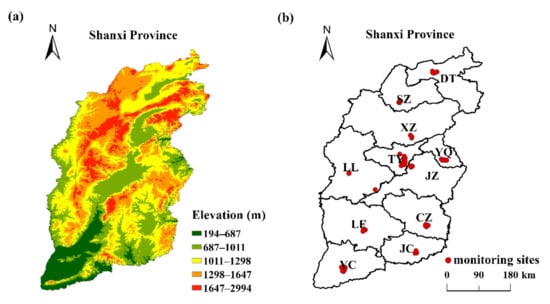
Figure 1.
The terrain of Shanxi Province (a) and the geographical locations of the prefecture cities in it with the monitoring stations being marked with red dots (b).
As Shanxi Province is located in the mid-latitude inland on the east coast of the mainland and blocked by the eastern mountains, the climate is weakly affected by the ocean, and the climate type belongs to a temperate continental monsoon climate. The annual average air temperatures in different places range from 3 to 14 °C. The temperature difference between day and night is large, and so is that between the northern area and southern area. In general, the temperature increases from north to south, and from basins to mountains.
The prevailing wind is northwest in the northern part of Shanxi, northeast in the central region, southwest and southeast in the southern part. CZ and LL had the highest annual average wind speeds, being 3.15 m/s and 2.81 m/s, respectively. The average annual wind speeds in LF (1.47 m/s) and SZ (1.62 m/s) and LL (1.98 m/s) were smaller than 2 m/s, while the speeds in the rest cities were in the range of 2.03 to 2.43 m/s. For the seasonal change, the wind speed at each studied city was the largest in spring, while had no obvious difference in other seasons (Table S1).
The annual average precipitation in the prefectural cities of Shanxi is between 200 and 600 mm, and highly concentrated in summer from June to August, which accounts for more than 60% of the year. In general, precipitation is conducive to the removal of NO2 in the atmosphere, however, when the skies pulse with lightning on rainy days, N2 will react with O2 to form NOx. The precipitation and lightning mainly concentrate in summer. Among the 11 prefectural cities, JC had the largest rainfall throughout the year (572.60 mm) and also in spring (202.20 mm) and winter (23.60 mm), XZ had the second largest precipitation throughout the year (536.82 mm) and the largest rainfall in the summer season (403.40 mm), while YC had the largest rainfall in autumn (109.90 mm). The seasonal averages of wind speed, temperature and precipitation are summarized in Table S1.
Overall, the soil in Shanxi Province is relatively infertile due to its being located in the Loess Plateau with a low amount of precipitation and low frequencies of lightning and forest fire. Therefore, the natural NOx emission should be limited in this area.
The industries in Shanxi are dominated by heavy industries such as coal mining, coking, steelmaking, thermal power generation, cement production, and alumina production. In 2018, the overall output of coal was 962.34 million tons, coke 92.56 million tons, crude steel 53.86 million tons, steel products 49.03 million tons, electricity 308.76 billion kwh, cement 43.77 million tons, and alumina 20.25 million tons [26]. In terms of the regional distribution, coal mining is mainly concentrated in SZ and DT in the north of Shanxi, LL in the middle, and CZ in the south; coking and steelmaking are mainly concentrated in the central and southern regions; power production is mainly concentrated in the north, but industrial power consumption is concentrated in the central and southern regions; cement production is also concentrated in the central and southern regions except DT in the north (Figure 2). For the population, TY, YC, YQ, CZ, JC and DT have a relatively high density (Figure 2). Because of the extremely cold and long winters, a central heating supply policy is implemented in Shanxi, which begins on November 1 in every year and ends on March 31 of the following year. We defined this period as the “heating period”, while the other time (from April 1 to October 31) in the year is defined as a non-heating period. Central heating is mainly supplied by burning coal and is therefore an additional important source of air pollution during heating periods in Shanxi.

Figure 2.
The spatial distribution of population and various industrial development indicators in Shanxi Province. The data are from Shanxi Statistical Yearbook-2018 [26].
2.2. Data Sources
The real-time concentration data of six criteria pollutants (NO2, PM2.5, PM10, SO2, CO and O3) monitored at the state controlling air sampling (SCAS) sites located in each city were downloaded from the website of China National Environmental Monitoring Center (CNEMC, http://www.cnemc.cn/, accessed on 8 November 2021). This dataset has been applied in many previous studies [24,27,28] to investigate the temporal and spatial variations of the gaseous and particulate pollutants in China [19,25,28,29]. The arrangement principle of the sampling sites and the automated monitoring systems used have been introduced in detail by Zhao et al. (2016) [19]. There is a total of 57 SCAS sites in Shanxi, among which eight sites were set up in TY; four sites in JZ; six sites in DT, LF, YQ and JC, respectively; five sites in CZ, SZ and YC, respectively; and three sites in XZ and LL, respectively (Figure 1b).
The concentrations of NO2 at the SCAS sites were measured according to the Ambient Air—Automatic Determination of Nitrogen Oxides-Chemiluminescence method (HJ 1043-2019) issued by the Ministry of Ecology and Environment of the People’s Republic of China in 2019 [30]. In brief, the sample air was first divided into two paths after entering the measurement instruments. One path measured the concentration of NO directly. The NO in the reaction chamber was oxidized by excess O3 to form an excited state nitrogen dioxide molecule, which emits light during the process of returning to the ground state. Within a certain concentration range, the concentration of NO in the air is proportional to the light intensity. The other path was to convert NO2 into NO through a molybdenum conversion furnace and then measure the concentration of NO to give the total NOx. The concentration of NO2 can be determined by subtracting the concentration of NO from the concentration of total NOx.
2.3. Statistical Analysis
In this study, one-year hourly measurement from 1 January 2018 to 31 March 2019 was chosen to do the monthly variation analysis, while that from 1 March 2018 to 28 February 2019 was used to do the rest analysis. Before publication, the data had been validated based on Technical Guideline on Environmental Monitoring Quality Management HJ 630–2011 [31] which mainly targets the data with too short sampling time (<45 min in an hour) and the anomaly with higher concentrations of specific pollutants [19]. In this study, the data missing problem was further handled based on China National Ambient Air quality Standard (NAAQS) (GB 3095-2012) [32]. The valid 24-h average concentration requires at least 20 hourly mean values for NO2, CO, SO2, PM10, PM2.5, and the 8-hour average concentration requires at least 6 hourly mean values for O3. For all the six pollutants, the monthly average and the annual average concentration requires at least 27 (25 in February) and 324 daily mean values respectively. If these rules were met, the partial missing of the data was acceptable.
Because there were also some other inevitable problems such as consecutive repeats and severe outliers, the data were then processed by us following the methods reported by Zhai et al. (2019) and Lu et al. (2018) to ensure their validity [25,29]. For consecutive repeats, the values were removed from the hourly time series when there are > 24 consecutive repeats [25]. To identify the outliers, all hourly data were standardized by the z-score standardization, then the standardized data(zi) were marked as outliers and removed if they met one of the following criteria: (1) zi is larger than 4, i.e., |zi|>4; (2) the enhancement of zi compared to the previous hourly value is larger than 9, i.e., |zi − zi-1|>9; (3) the ratio of the value to its centered rolling moving average of order 3 larger than 2, i.e., 3zi/(zi-1 + zi + zi + 1) > 2 [12]. After processing, an average of 335 daily data and 12 monthly data were obtained in each city in the investigated year.
The citywide average concentrations were calculated by averaging the concentrations at all sites in each city, and then the daily average, monthly average, quarterly average and annual average were calculated for the subsequent analysis and comparison. The averaging formula is:
is the average concentration of pollutants in each city, n is the number of monitoring sites in each city, and xi is the hourly concentration value uploaded by each monitoring site.
The spatial distribution map of NO2 was draw via Kriging method of the Geography Information System (GIS) module in Globalization Modeling System (GMS) software, which is an interpolation algorithm that creates a raster surface based on known point values. The brief formula is:
xi is a series of known observation points on the space area, and z(xi) is the concentration value of NO2, z*(x0) is the corresponding value at the non-observed point x0. λi is the weight coefficient, which needs to meet the following two criteria, unbiasedness () and minimum estimated variance ().
Other analytical methods are introduced as follows.
2.3.1. Local Spatial Autocorrelation Analysis
Spatial autocorrelation analysis methods have been used to investigate whether the observed attribute value of a variable (e.g., concentrations of pollutants like NO2, SO2, etc.) in one area is correlative of attribute values of the variable in its surrounding areas [33]. The methods for calculating spatial autocorrelation can be categorized into two types, global spatial autocorrelation analysis and local spatial autocorrelation analysis [24]. Global spatial autocorrelation analysis is to research the spatial distribution of the observed attribute values of the variable in the entire region. Local spatial autocorrelation analysis can be used to determine local spatial clusters of high or low observed attribute values of the variable in the studied areas, reflecting the correlation between a local area and surrounding areas.
In this study, we selected global Moran’s I as the indicator to analyze the global spatial autocorrelation, then Anselin’s Local Indicator of Spatial Association (LISA) represented with Local Moran’s I and Moran’s I scatter plot were selected as the indicators of local spatial autocorrelation. LISA could localize the presence and importance of spatial autocorrelation based on measures [16,34,35]. That is, LISA play a role in the identification of hot spots-areas where the considered specific phenomenon is extremely marked across localities as well as spatial outliers [34,36]. Moran’s I scatter plot is also generally used to illustrate spatial correlations among regions, which could conduct a more disaggregated comment to the type of spatial autocorrelation that exists in the observed data [34,37].
The Global Moran’s I is calculated using the following formula:
The Local Moran’s I is calculated using the following formula:
where n is the sample size, xi and xj denote the attribute values of spatial areas i and j, here it’s the concentration of NO2 in each city,
represents the mean value of all spatial areas, S2 represents the variance of the attribute value of spatial areas, Wij is the spatial weight coefficient matrix, which represents the adjacent relationship of each spatial area. We got Wij with OpenGeoDa v1.2.0, a free software, developed by the Center for Spatially Integrated Social Science (University of California, Santa Barbara, CA, USA) based on ESRI’s (Environmental Systems Research Institute, Redlands, CA, USA) MapObjects LT2 technology. Ii ranges from −1 to 1. When Ii > 0 (Ii < 0), the study entire area presents a positive (negative) spatial autocorrelation in the spatial distribution, and the observed attribute value of entire area presents a clustered (discrete) spatial pattern; when Ii is close to 0, there is no spatial autocorrelation of observed attribute value, and they are randomly distributed in space. When Ii > 0 (Ii < 0), there is a strong positive (negative) spatial autocorrelation between the observed attribute values of the regional spatial area i and that of the surrounding spatial areas, showing a local spatial aggregation (discrete).
To ensure the correctness of the inferred conclusion under a certain probability, this study conducted a randomness test on Global Moran’s I (I) and Local Moran’s I (Ii):
Zi is the normalized form of observations in area i and represents the significance level of spatial autocorrelation, E(I) represents the mathematical expectation of Global Moran’s I or Local Moran’s I, and VAR(I) represents the variance.
Moran’s I scatter plot is constructed based on the idea of regression of Global Moran’s I with the following formula:
where Z is the vector of Zi, the slope parameter I is the Global Moran’s I, and WZ is the spatially lagged variable (NO2 in this study). Thus, a Moran scatter plot can highlight cells with anomalous levels of spatial autocorrelation by plotting the location of WZ with respect to Z and adding a regression line (Global Moran’s I). In this study, the computing and graphical displays were done using R Studio with additional package of “spdep” [38].
2.3.2. Back Trajectory Analysis
In this study, 48 h backward trajectories arriving at the most polluted monitoring site of each prefectural city with an initial height of 100 m above ground level were calculated using reanalysis data from National Centers for Environmental Prediction [39]. The calculation was performed using MeteoInfo-TrajStat [40]. The UTC time 00, 02, 04, 06, 08, 10, 12, 14, 16, 18, 20, 22, were set as the start time of the trajectories. Then, the trajectories having similar geographic origins and histories in one season were clustered into groups, and the mean trajectory for each group was calculated. The detailed principles and methods were similar to those reported by Squizzato and Masiol [41].
2.3.3. Concentration Weighted Trajectory (CWT)
To localize major sources of NO2 in each prefectural city, the CWT was calculated on a 0.5° × 0.5° resolution by combining the concentration of NO2 with the above calculated backward trajectories. The range of the study domain was in 34–41° N and 110–114° E. The CWT for NO2 for a particular grid cell (i, j) is determined by using the following averaging formula [42]:
where CWTij is the weighted average concentration of grid ij; N is the total number of trajectories; k denotes a trajectory; Ck denotes the concentration observed on the arrival of trajectory k at the receptor, and τijk is the duration in which trajectory k stays in grid ij. As CWT is a conditional probability function, like any other air-quality models, some uncertainties exist in the results modeled by CWT inevitably. When the airflow retention time in each grid is short, the CWT value will fluctuate greatly to increase the uncertainty, and when Nij (the total number of back-trajectory segment endpoints that fall into the grid cell (i, j) during all days) is very small, high CWTij value will be generated. To eliminate this uncertainty, the CWT values were multiplied by an empirical weight function W(ij), which was defined as follows [43]:
3. Results and Discussion
3.1. NO2 Pollution Level
In 2018, the concentration of NO2 in most of the prefecture-level cities in Shanxi ranked the top heavy-polluted cities in China according to the study of Shen et al. [44]. As shown in Table 1, the annual average concentrations of NO2 in the prefectural cities of Shanxi mainly distributed in the range of 28.84–48.93 μg/m3. In TY, LL, YQ, JZ and XZ, the values exceeded the grade 2 maximum allowable mass concentration value (40 μg/m3) (GB3095-2012) required by the Chinese National Ambient Air Quality Standards (NAAQS).

Table 1.
Pollution Situation of NO2 in prefecture Cities of Shanxi Province.
TY had the largest number of over-standard days (the second-level daily upper limit of NO2 is 80 μg/m3 according to GB3095-2012, which accounted for 6.71% of the total days in the year, respectively. The maximum daily average concentration in TY reached 107.28 μg/m3 on 11 January 2019. On this day, the air pressure and temperature were very low, the relative humidity was 65.25%, southeast, south, and southwest were the prevailing wind direction. Because the most polluted cities in Shanxi with large amounts of air pollutants emissions from coking industries and residential coal combustion are all gathered in the southwest direction of TY, we deduced that regional transportation from those cities was the major reason resulting in serious pollution in TY. In LF, JZ, YC and XZ, the highest daily average concentration exceeded 90 μg/m3, but lower than 100 μg/m3. The over-standard days were all concentrated in the heating season, and the highest over-standard rate occurred in TY (15.60%), followed by LF, XZ, JZ and YQ (9.86%, 9.15%, 8.45% and 7.75%, respectively). The above results indicated that combustion for heating in cold days was a predominant factor causing NO2 pollution in Shanxi.
The NO2 concentration displayed an obvious seasonal variation with minimum value in summer and maximum value in winter in all the cities except LL, in which NO2 concentration was comparable in spring, summer and autumn. A more detailed analysis showed that the seasonal over-standard situation was different in different cities (Table 1). TY, LF, YQ and JZ exceeded the standard most severely in winter, followed by autumn. XZ exceeded the standard most severely in winter, followed by spring and autumn. In JC and YC, there were only some days in winter exceeding the standard. In CZ, there were only some days in autumn exceeding the standard. Although the annual average concentration of NO2 in LL city exceeded the second-level annual upper limit and ranked second in the province, no one day exceeded the daily average concentration limit (80 μg/m3). This phenomenon implies that simply pursuing meeting the standard in each day cannot ensure that the annual average meets the standard. Therefore, an integrated planning and detailed technical scheme towards the two goals is necessary for the government to control the air pollution. The first thing the government needs to do is develop a highly detailed and high-resolution NOx emission inventory and calculate out the total amount of emission reductions needed to fulfill the above two goals. Based on that, the pre-control sources and industrial enterprises can be determined according to their emission amounts, while the total amount of emission reductions needed to control can be apportioned to all of the pre-control sources and industrial enterprises after taking into account the emission mitigation potential and maturity of the emission reduction technologies for each source, as well as the economic costs for the enterprises and the government.
In addition, we found that the cities with the least precipitation in spring, autumn and winter tend to have higher concentrations of NO2, for example, spring in TY, autumn in XZ and TY, and winter in TY and XZ. The cities with higher speed had low NO2 concentrations such as CZ and DT.
3.2. NO2 Monthly Variations
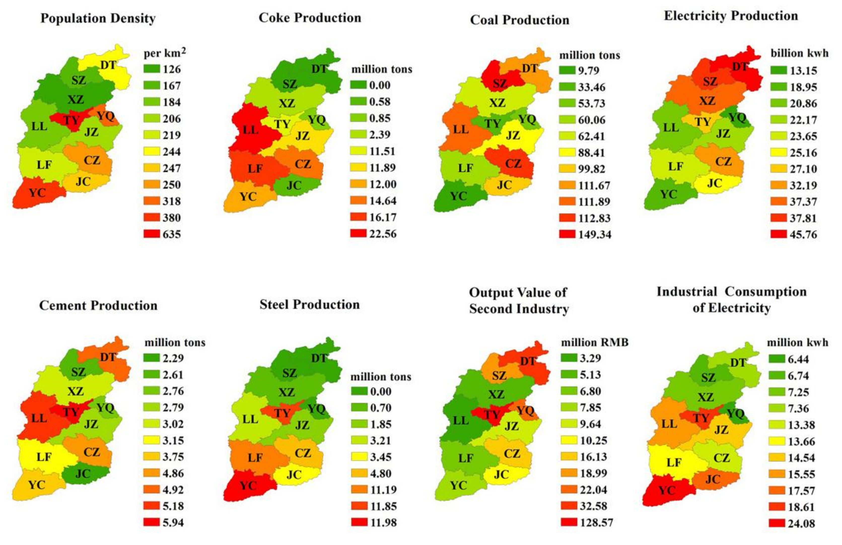
As shown in Figure 3, the monthly variations of NO2 concentration in the prefecture cities in Shanxi can be classified into four types. Six cities (CZ, LF, YQ, SZ, JZ and YC) belonged to the first type,”winter unimodal” (Figure 3a). For this type, the peak of NO2 concentration usually occurred in January. The period from August to January was the rising stage, while that from January to August was the declining stage. The range (max-min) of monthly average concentration reached up to 40~60 μg/m3. This is a universal phenomenon in northern China as that found by Tian et al. [20]. The minimum in summer is usually benefit from the active chemical reaction, stronger vertical convection, and wet deposition. The maxima in winter can be mostly attributed to residential heating emissions, longer lifetime and meteorology, including shallower mixing depth, lower precipitation, and increased stagnation in winter [25]. Due to better diffusion conditions, the NO2 concentrations in all the cities in December of 2018 were obviously lower than those in November and January in the next year. From Figure 2, we can see that there were more heavy air-polluting industries and population in the cities of this type, indicating that NO2 pollution was mainly controlled by industrial emissions besides residential coal combustion emissions in winter.
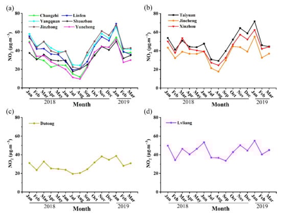
Figure 3.
Annual variations of monthly mean concentrations of NO2 in 11 prefecture cities in Shanxi Province. (a) first type; (b) second type; (c) third type; (d) fourth type.
The representative cities of the second type were TY, JC and XZ (Figure 3b). The difference between this type and the first type was that the NO2 concentration had a plateau or small fluctuation in spring, which maybe resulted from the increase of soil NOx emissions as the temperature increases. Compared with the cities in the first type, the cities in the second type suffered less influence from industrial emissions, but more from traffic exhaust and soil emissions. As the capital of Shanxi Province, TY has the highest population density among all the prefectural cities (Figure 2) and the highest car ownership, while most of the industries in the urban area of TY have been relocated to the outer suburbs or farther afield. JC has a relatively high population density (Figure 2) and is actively building a livable city. The economy of XZ has always been underdeveloped with less polluting industries, but the air quality can be influenced by the regional transportation of air pollutants from the surrounding polluted cities like Taiyuan, which was discussed further in Section 3.6. In addition, the whole greening rate in these three cities is relatively high.
DT was marked as the third type (Figure 3c). The difference between this type and the above two types was that the change of NO2 concentration throughout the year was relatively small with the concentration being only about 10 μg/m3 higher in winter than other seasons. In recent years, DT has successfully transformed from a heavy industry city into a tourist city with many pollutant sources being controlled. This effort, coupled with a relative low air temperature, which can inhibit the soil emission in spring and NO2 degradation in summer, leads to a relatively low concentration of NO2 (monthly averge < 40 μg/m3) and small fluctuations over the whole year. LL appeared as the fourth type—“summer and winter bimodal” (Figure 3d) with the summer and winter peak basically the same. However, the overall change of NO2 concentration throughout the year was small with less than 20 μg/m3 difference among the monthly averaged concentrations. A faster rise of NO2 concentration in LL from April to June than that in other cities implied a higher impact from soil sources, while the lower concentration in winter than most other cities can be attributed to good diffusion conditions with open terrain and a high altitude. Although the heating activities in winter could result in higher pollutant emissions than summer, more times had higher speed of wind in winter than in summer, and the average wind speed was also higher than that in summer, so the pollutants were not easy to accumulate (Figure S1).
Overall, due to the influence of coal combustion for heating in winter, each city had a winter peak. Besides that, NO2 concentration in the first-type cities was mainly controlled by industrial sources, while the second-type cities should be mainly controlled by traffic exhaust. Soil NOx emissions might have a certain impact on the NO2 level in the second- and forth-type cities, resulting in a summer peak in those cities. Under low emission and low air temperature conditions like in DT, not only was the concentration of NO2 low, the fluctuation was also small across the whole year. The comparable peak values in summer and winter in LL might be associated with the high impact from soil sources in summer and good diffusion conditions in winter.
3.3. NO2 Diurnal Variations
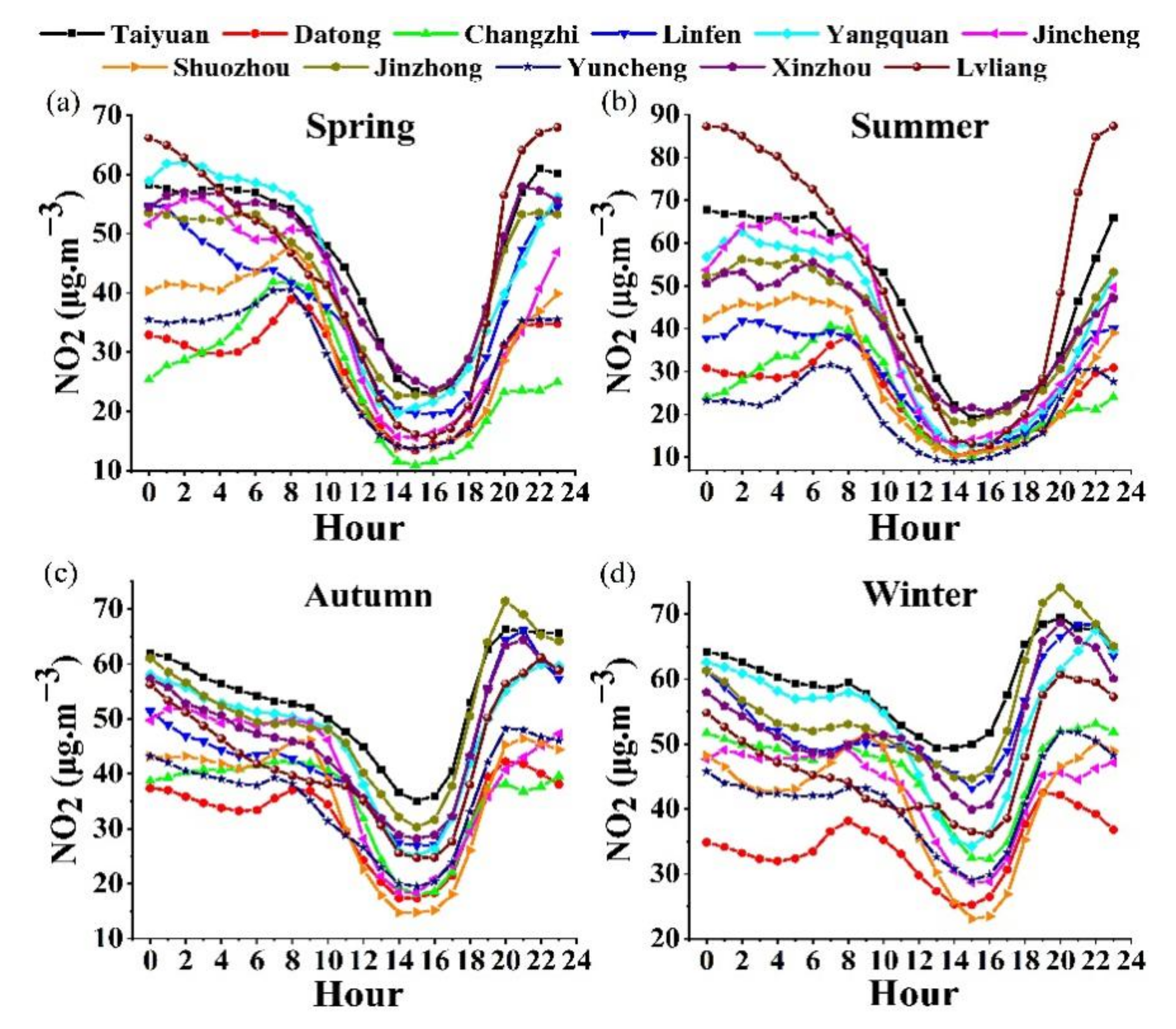
The diurnal variation of NO2 in different prefecture cities of Shanxi Province was generally consistent. As can be seen from Figure 4, the concentration of NO2 in a day was lowest in the afternoon, one main reason is it will be consumed by the photochemical reaction when it is exposed to strong solar radiation except for strong vertical convection in that time. The duration of the minimum concentration of NO2 in one day in each season was also related to the solar radiation. It lasted the longest time (12:00 am to 6:00 pm, a total of 7 h) in summer, followed by the spring (1:00–5:00 p.m., a total of 5 h), while it could only last about 3 h in autumn and winter (2:00–4:00 p.m.). Taking the concentration in the morning as the reference, the decline of the NO2 concentration in the afternoon was always large in spring and summer, while small in autumn and winter, further indicating that solar radiation has a great influence on NO2 concentration.
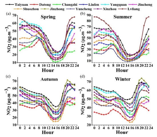
Figure 4.
Diurnal variations of hourly mean concentrations of NO2 in 11 prefecture cities in Shanxi Province. (a) spring; (b) summer; (c) autumn; (d) winter.
When the solar radiation becomes weaker, the effects of anthropogenic emissions as well as decreasing boundary layer thickness will start to stand out. During the late afternoon fresh emissions of NO reduce ozone and the ozone reaction with NO produces more NO2, leading to rapid rise of NO2 concentration in the atmosphere, so the NO2 pollution in the evening was the most severe with the concentration reaching the peak at around 9:00 p.m. in fall and winter, and later (midnight) in spring and summer with few exceptions. In spring, autumn and winter, the NO2 concentration would slowly decrease or remain stable from about 12 o’clock in the middle of the night to about 5 or 6 o’clock in the morning. Afterwards, it increased gradually with a small peak appeared at 8~9 a.m. in some cities. This phenomenon can be observed mainly in DT, SZ, CZ and YC, while it was not very obvious in other cities. From Figure 2 we can see that, DT, CZ and SZ are the main coal production bases. The mined coal is mainly transported by diesel-powered heavy trucks from mine areas to other places. Since 2013, in order to control the impact of diesel vehicle exhausts on the air quality, Shanxi Province has imposed restrictions on the running period of diesel vehicles on roads in and around each city, which are open from 12 PM to 6 AM in the next day while forbidden during the daytime. The transportation of the diesel vehicles at late-night will inevitably discharges a large amounts of NO. After sunrise, already high O3 concentration in the air (Figure S2) plus the supplement of O3 from the upper air by convection [45] promotes the titration of NO by O3 rapidly and resulted in a rapid increase of NO2 concentration in the early morning. Because some industrial production activities are stronger at night than those in the daytime, leading to larger amounts of NO emission at night, which may be the main reason for the morning peak of NO2 level in the industrial city-YC. In the cities of Shanxi Province, the time of maximum NO2 in the morning didn’t obviously lag behind the traffic-rush hour, indicating that the traffic exhaust during the morning commute might have a low impact on the concentration of NO2 in the atmosphere.
In summer, the NO2 concentration would increase at 3 o’clock in the middle of the night in most of the prefecture cities except DT, which was significantly earlier than other seasons. It should be pointed out that not all of the cities had the morning peak. The variation was more complex in the nighttime among different cities due to different terrain and associated evolution of meteorological conditions.
3.4. The Spatial Distribution and Local Spatial Autocorrelation of NO2
3.4.1. Spatial Distribution
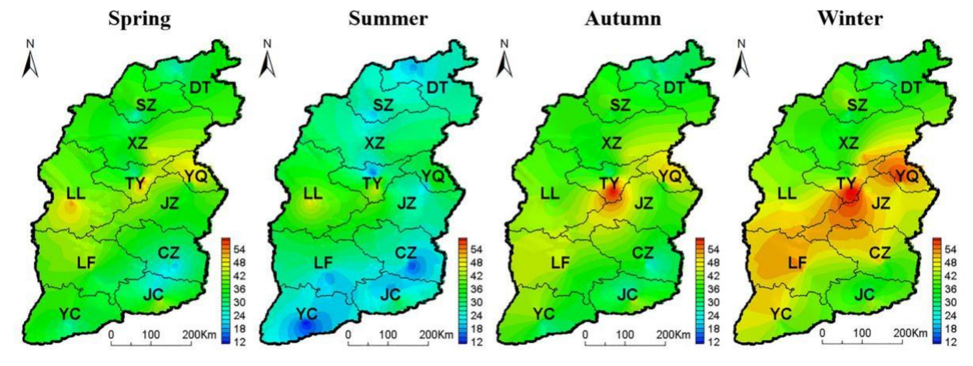
Although NO2 is an important precursor of PM2.5 and O3, but interestingly, there are large differences among their spatial distribution characteristics (Figure S2). The regions having high PM2.5 concentrations mainly concentrated in the southern Shanxi including LF, YC and JC, followed by central cities like TY and YQ (Figure S2). The regions having high O3 concentrations also concentrated in the southern cities (LF, JC, YC, CZ) and the central city—TY (Figure S2). However, the regions having high NO2 concentrations mainly concentrated in the central part of Shanxi and trended on the whole from southwest to northeast (LL/LF–TY/JZ–YQ/JZ) (Figure S2 and Figure 5). Northern DT, southern YC, and the central areas of JC and CZ were the areas where the NO2 pollution were lightest (Figure 5). The study by Shen et al. (2020) also observed the similar phenomenon [44].
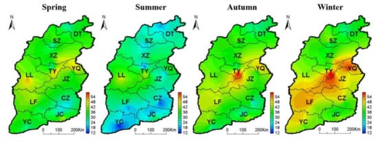
Figure 5.
The spatial distribution of NO2 in different seasons of Shanxi Province.
Combining the spatial distribution of the population and various industry development indicators in Shanxi Province (Figure 2), we can deduce that coke production should be the major source of NO2 in LL, LF and western JZ, which also caused heavy pollution of SO2 in these areas. As the capital city of Shanxi Province, the anthropogenic emissions especially mobile emissions are high in TY due to the dense population and intense human activities, thus the NO2 pollution is serious. The steel and cement production should be additional important sources of NO2. Although the industry production displayed in Figure 2 ranked low in YQ compared with other cities, the production of refractory materials is prevalent with high-temperature combustion of natural gas, which extremely favor the formation of thermal NOx. One more fact that cannot be ignored is YQ is an important transmission corridor of air pollutants between TY and Shijiazhuang (the capital city of Hebei) with about 100 km away from either one of the cities, both of which have heavy NO2 pollution [44] and thus have high probability to aggravate NO2 pollution in YQ through air mass transportation. From Figure 2, we can see that although the electricity production of DT ranked first, the pollution of NO2 was light, so was SZ. This may be due to the fact that the emission limits of air pollutants in the electricity industry are very rigid in China.
From the perspective of seasonal changes, winter was the most polluted season of the year, followed by autumn and then spring, while summer was the least polluted season. The pollution degree in TY and JZ in autumn was close to that in winter, but the pollution range was smaller than that in winter. The heavy pollution of NO2 in winter was closely related to the residential coal combustion for heating.
3.4.2. Spatial Autocorrelation
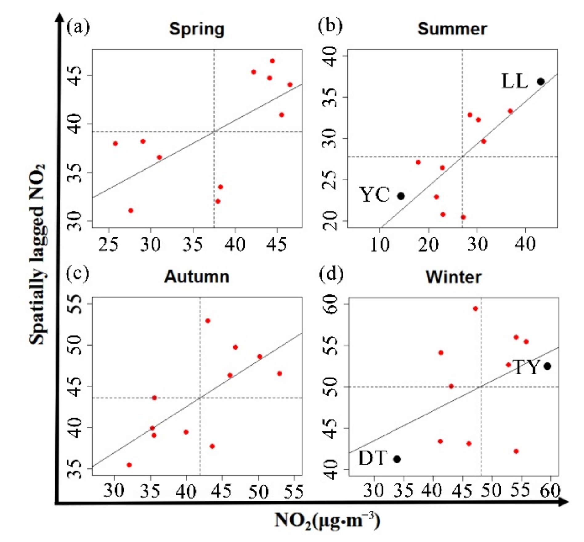
In Figure 6, the slope of the regression line represents the value of Global Moran’s I. A positive value indicates that the entire study area exhibited positive spatial autocorrelation in the spatial distribution. All regression lines have positive values in all of the four seasons, indicating that NO2 presented a clustered spatial pattern in the whole year.
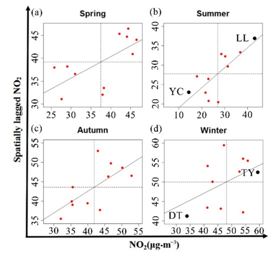
Figure 6.
Moran scatter plots of seasonal mean concentrations of NO2 in 11 prefectural cities in Shanxi Province. (a) spring; (b) summer; (c) autumn; (d) winter.
Moran’s I scatter plot includes four quadrants. Among them, Quadrant 1 (High value next to High, H-H) and Quadrant 3 (Low value next to Low, L-L,) represent positive spatial autocorrelations which include “hot spot” and “cold spot”, that means where the attribute value is high, the surrounding attribute value is also high, and where the attribute value is low, the surrounding attribute value is also low. Quadrant 2 (high amongst low, H-L) and Quadrant 4 (low amongst high, L-H) represent negative spatial autocorrelation, and that means where the observed value shows a high attribute value, the surrounding attribute value is low, and the surrounding attribute value is high where the attribute value is low [35,37,46]. In Shanxi, most dots are located in Quadrant 1 and Quadrant 3 (Figure 6), implying that there were only two spatial clustering types, H-H and L-L. In the subgraphs of Figure 6, the locations with significant LISA statistics (Local Moran’s I) were marked with black dots in the corresponding Quadrant. In winter, LISA statistics is significant in TY (Figure 6d), suggesting that it was the hot spot of NO2 pollution in Shanxi in this season. That is, not only was TY itself heavily polluted, but the surrounding cities connected to it were also heavily polluted. LL was a hot spot in summer (Figure 6b). On the contrary, YC was a cold spot area in summer (Figure 6b), suggesting that the city as well as its surrounding areas had low NOx pollution in this season. In winter, the area centered on DT belonged to the cold spot area (Figure 6d). The data in the past bulletins of the environment state in Shanxi Province showed that comprehensive air quality index in DT rose from bottom in 2008 to the top in recent years. The environmental air quality has been greatly improved, and the pollution control effect is obvious. In spring and autumn, there was neither hot spot nor cold spot (Figure 6a,c).
3.5. Correlation between NO2 and Other Contaminants
3.5.1. The Roles of NO2 in O3 and PM2.5 Pollution
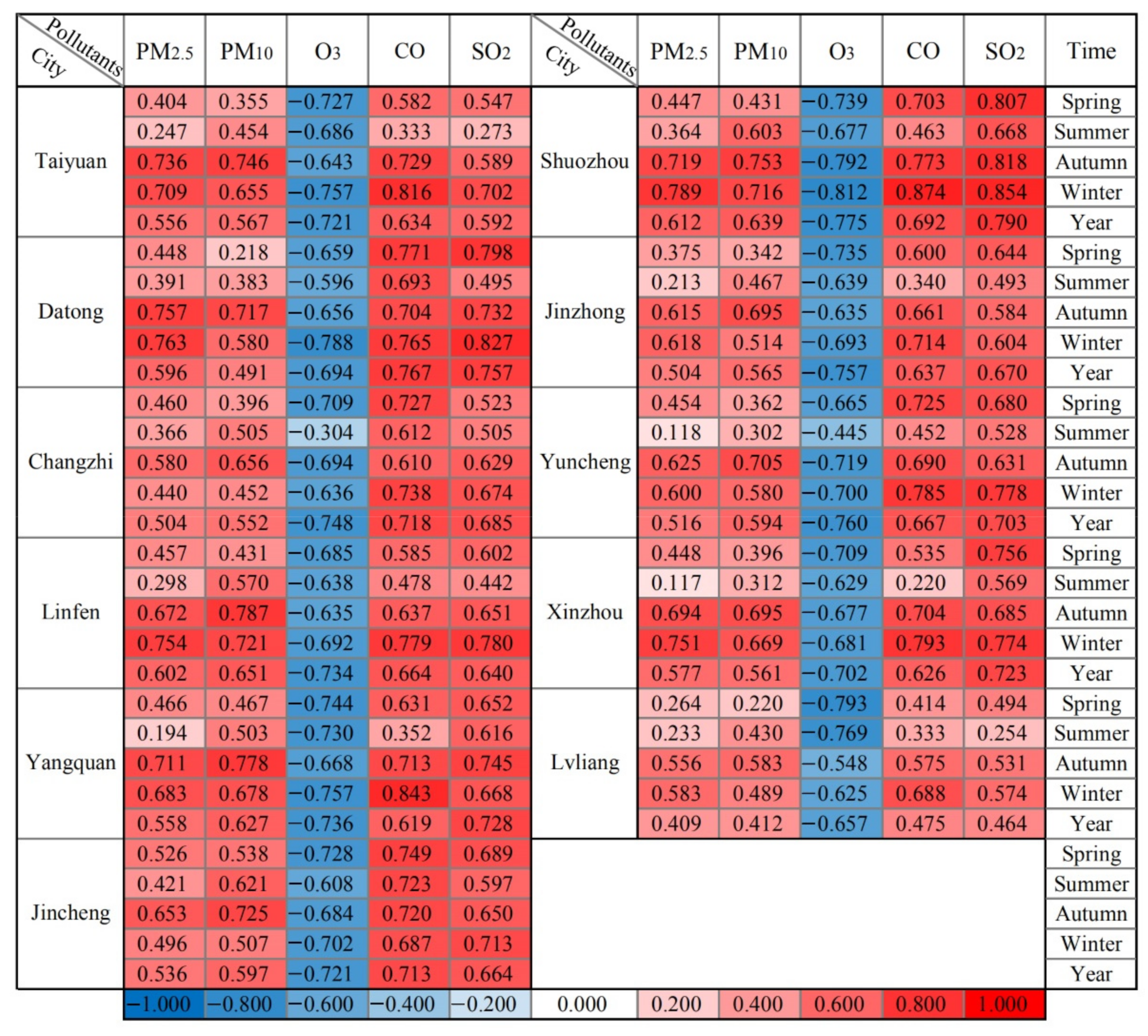
NO2 is considered to be an important precursor of atmospheric O3 and PM2.5. In all of the cities, NO2 showed a strong negative correlation with O3 (Figure 7). Wang et al. (2019) found that most northern cities in China have negative correlations between NO2 and O3 but positive correlations in southern cities [24], indicating that NO2 played different roles in the generation of O3 in different regions. Although O3 pollution mainly happened in summer with NO2 being an important combustion improver, no significant seasonal difference was observed about their correlation coefficient (Figure 7). Some studies found that areas with higher NO2 concentrations tend to have lower O3 concentration in southeast China [20]. However, we cannot find the similar phenomenon in Shanxi, even in summer, which maybe attribute to variable industries, terrain, and meteorological conditions for the cities in it. From Figure S2, we can see that the places with higher O3 concentration are mainly concentrated in the south part of Shanxi with higher temperature and stronger solar radiation, while higher NO2 concentration are mainly concentrated in the central part of Shanxi with larger industrial emissions including coking production, electricity production and cement production etc. as shown in Figure 2. Similar spatial distribution between SO2 and NO2 can also illustrate this point. However, TY was an exception, where the concentrations of NO2 and O3 were both higher than its neighboring areas, but the concentration of SO2 was lower than the latter. The main reason is that TY has a very high population density (Figure 2) and car ownership, traffic should have a large contribution to NO2 pollution, which then resulted in heavy O3 pollution. In LL, which has a higher altitude, complex mountainous terrain and relatively lower air temperature, the concentration of O3 was low though the concentration of NO2 was high.
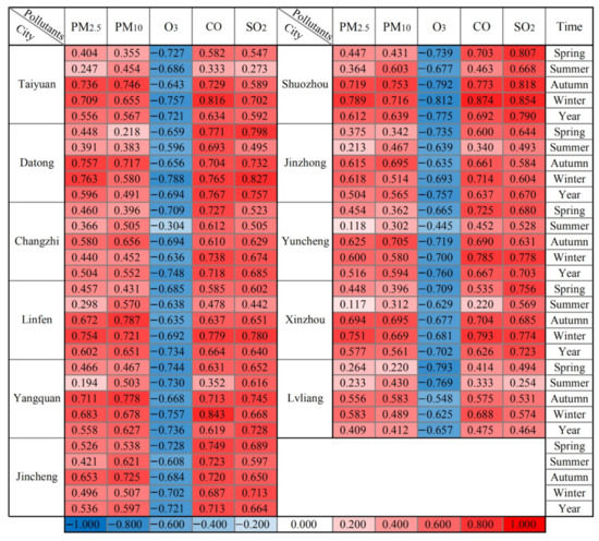
Figure 7.
Spearman’s correlation coefficient between NO2 vs. PM2.5, PM10, O3, CO and SO2. All data are statistically significant at the p = 0.01 level.
Opposite to O3, the correlation of PM2.5 with NO2 displayed a significant seasonal difference, which was much weaker in spring and summer than autumn and winter (Figure 7). This result indicated that the secondary conversion of NO2 in the atmosphere played more important roles in PM2.5 pollution in autumn and winter compared with that in spring and summer. Frequent dust events have a large contribution to PM in spring, which could weaken the association between PM2.5 and NO2. In summer, the weak correlation between PM2.5 and NO2 indicates that more NO2 take part in the formation of O3 but less participate in the process of PM2.5 formation. One possible reason is that strong solar radiation favors the photolysis of NO2 to yield more ground state oxygen atoms (O(3P)), which can react with O2 to produce more O3 [41]. The other possible reason is that the lower concentration of particles in summer results in higher actinic fluxes and heterogeneous HO2 radical loss, which further cause the accumulation of O3 in the atmosphere [21]. In autumn and winter, the photolysis rate of NO2 becomes slow. The high correlation between PM2.5 and NO2 implies that more NOx participates in the process of PM2.5 formation. It was reported that NOx could not only form nitrate directly, but also enhance aerosol-phase oxidation indirectly as a catalyst in heterogeneous processes, and as oxidants in aqueous reactions [21].
3.5.2. Air Pollution Type and Possible Sources
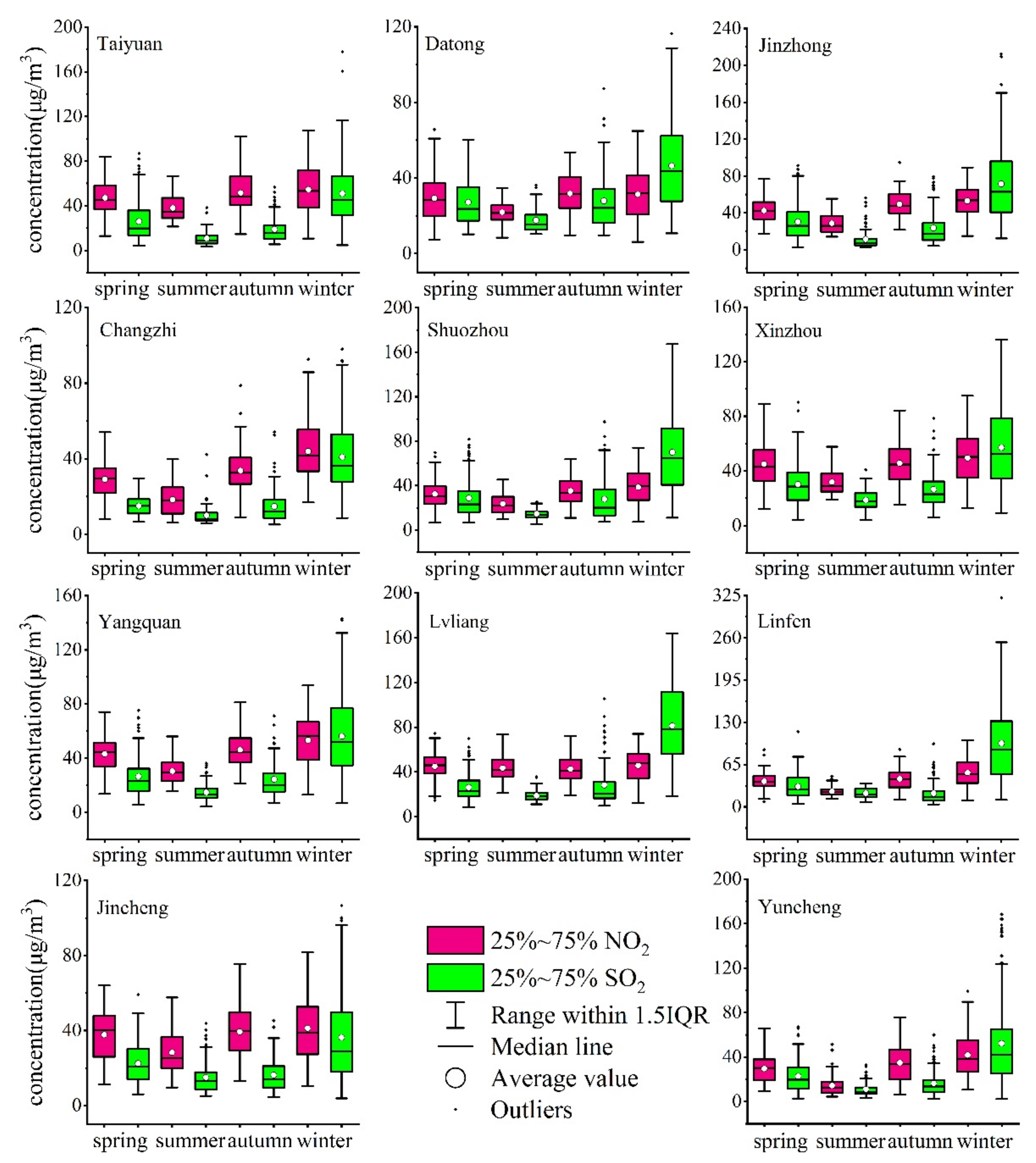
As a large coal producer, the air pollution of Shanxi province presented typical coal smoke pollution type for a very long time, with SO2 being the dominant atmospheric pollutant. The SO2 emission reduction was first emphasized by the Chinese government since 1995 [11]. After that, clear quantitative targets of reducing SO2 and NOx were set in China’s Five-Year Plans (FYPs), which was gradually tightened from the 10th FYPs (2001–2005) to the 13th FYPs (2016–2020) [5,11]. Especially since 2013, as the first national air pollution prevention and control strategy, the APPCAP for the first time sets out a road map for improving China’s air quality, proposing ten key actions and 35 specific measures in all aspects of air quality management [5,47]. The detailed measures targeting SO2 abatement included enforcing desulfurization in coal-fired power plants, restricting emission standards, improving fuel equipment, adjusting the energy consumption structure, reforming urban villages, switching from residential coal to cleaner fuels, promoting centralized heating system, removing small boilers, and eliminating small coking industries or reconstructing to large mechanized coke plants etc. [48,49,50,51].As a result, the concentration of SO2 in the atmosphere was decreasing prominently nationwide. However, NO2 pollution become increasingly prominent due to the lack of effective control policy and technology, as well as the drastic expansion of the public transportation system and vehicle numbers. Under this background, the pollution type in each city is re-evaluated in this study. From Figure 8, we can see that the concentration of NO2 was higher than that of SO2 in the whole year in four cities including TY, CZ, YQ and JC, displaying a traffic-related pollution type. In DT, SZ and LL, the concentration of NO2 was higher than that of SO2 in spring, summer, and autumn, but lower in winter, indicating that the coal smoke pollution type only occurred in winter in these cities. In JZ and XZ, the major difference from the above three cities were that the concentration of NO2 was close to SO2 in the seasons excluding winter. In spring and autumn of LF, NO2 had a higher concentration than SO2, but was opposite in winter and closed to each other in summer. In YC, NO2 had a higher concentration than SO2 in spring and autumn, while their concentrations in summer and winter were about the same. In LF and YC, both of which are located in the southmost part of Shanxi, with the highest temperatures among the 11 prefectural cities, the abnormally small difference between the two pollutants in summer compared with that in spring and autumn implies that NO2 has a higher degradation rate than SO2 under high temperature conditions. In winter, the increase of coal combustion emissions narrowed the gap between SO2 and NO2 concentrations, and even caused a reversal in most cities.

Figure 8.
Box plots of seasonal NO2 and SO2 concentrations in 11 prefecture cities in Shanxi province.
SO2 mainly comes from coal-fired emissions, while CO is related to incomplete combustion. In LL, NO2 had a weaker correlation with SO2 and CO, suggesting that non-coal-burning industries may contribute more to NO2 in this city (Figure 7). In SZ, the largest coal producer of Shanxi (Figure 2), NO2 had a strong correlation with SO2 and CO in most of the time in a year (Figure 7), suggesting that NO2 in this city mainly comes from the burning of residential coal. NO2 had a moderate correlation with SO2 and CO in the rest cities (Figure 7), suggesting that both coal burning and traffic exhaust play important roles in NO2 pollution in these areas. Due to the influence of residential coal combustion for heating, the correlation of NO2 with SO2 and CO was the strongest in winter, and the weakest in summer (Figure 7). In TY, YQ and JZ, NO2 had a strong correlation with CO, while having a moderate correlation with SO2 (Figure 7) in autumn and winter, implying a large contribution of motor vehicles in these two regions under low temperatures.
3.6. Regional Source
The potential source regions of NO2 in the cities which have over-standard days were shown in Figure 9, Figure 10, Figure 11 and Figure 12, while those in the cities having no over-standard days were shown in Figures S4–S7.
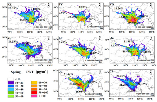
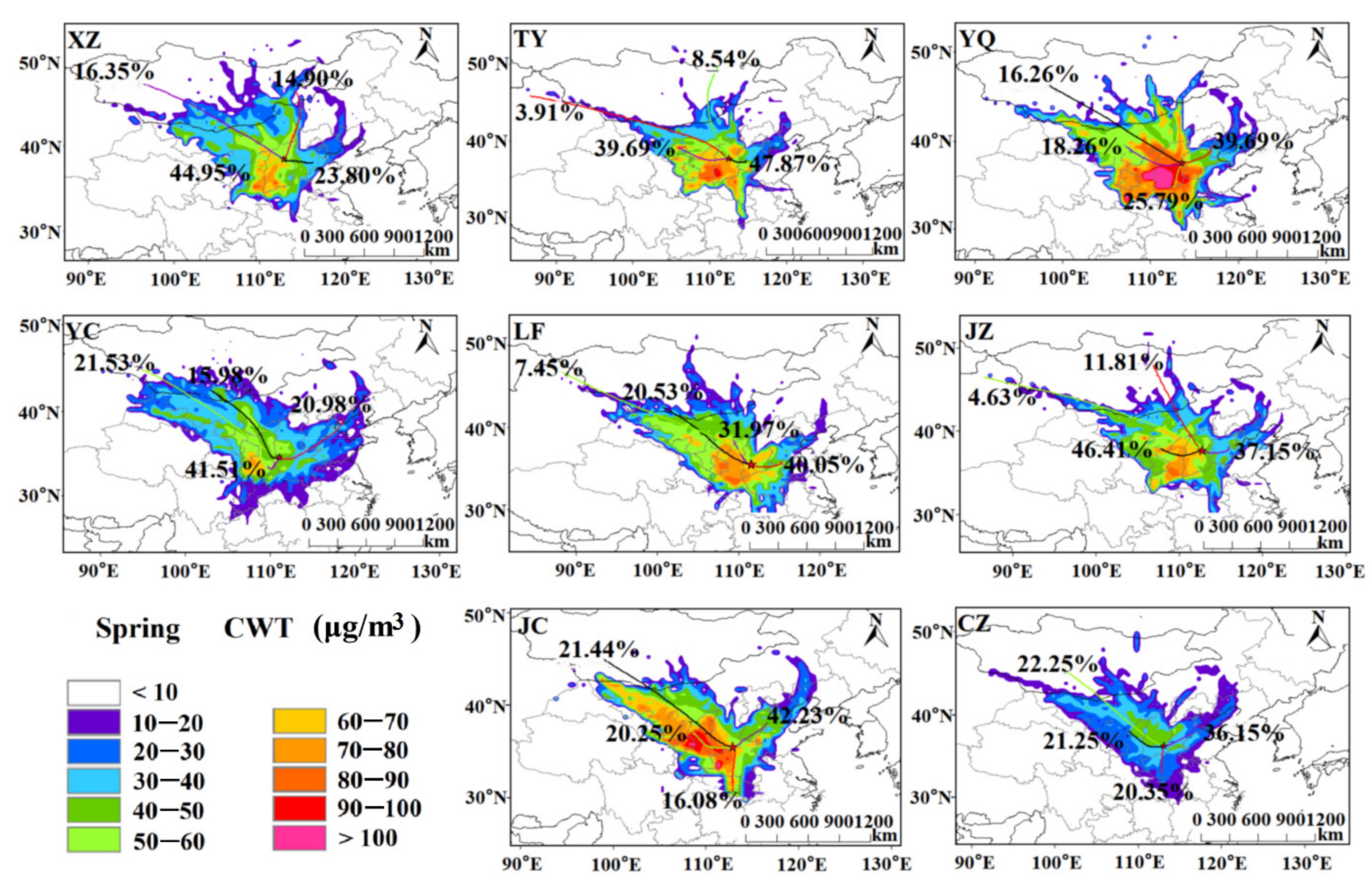
Figure 9.
CWT maps for NO2 by mass concentration (μg/m3) in spring in the cities having over-standard days.
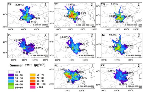
Figure 10.
CWT maps for NO2 by mass concentration (μg/m3) in summer in the cities having over-standard days.
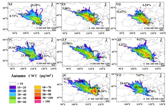
Figure 11.
CWT maps for NO2 by mass concentration (μg/m3) in autumn in the cities having over-standard days.
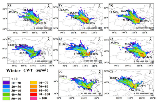
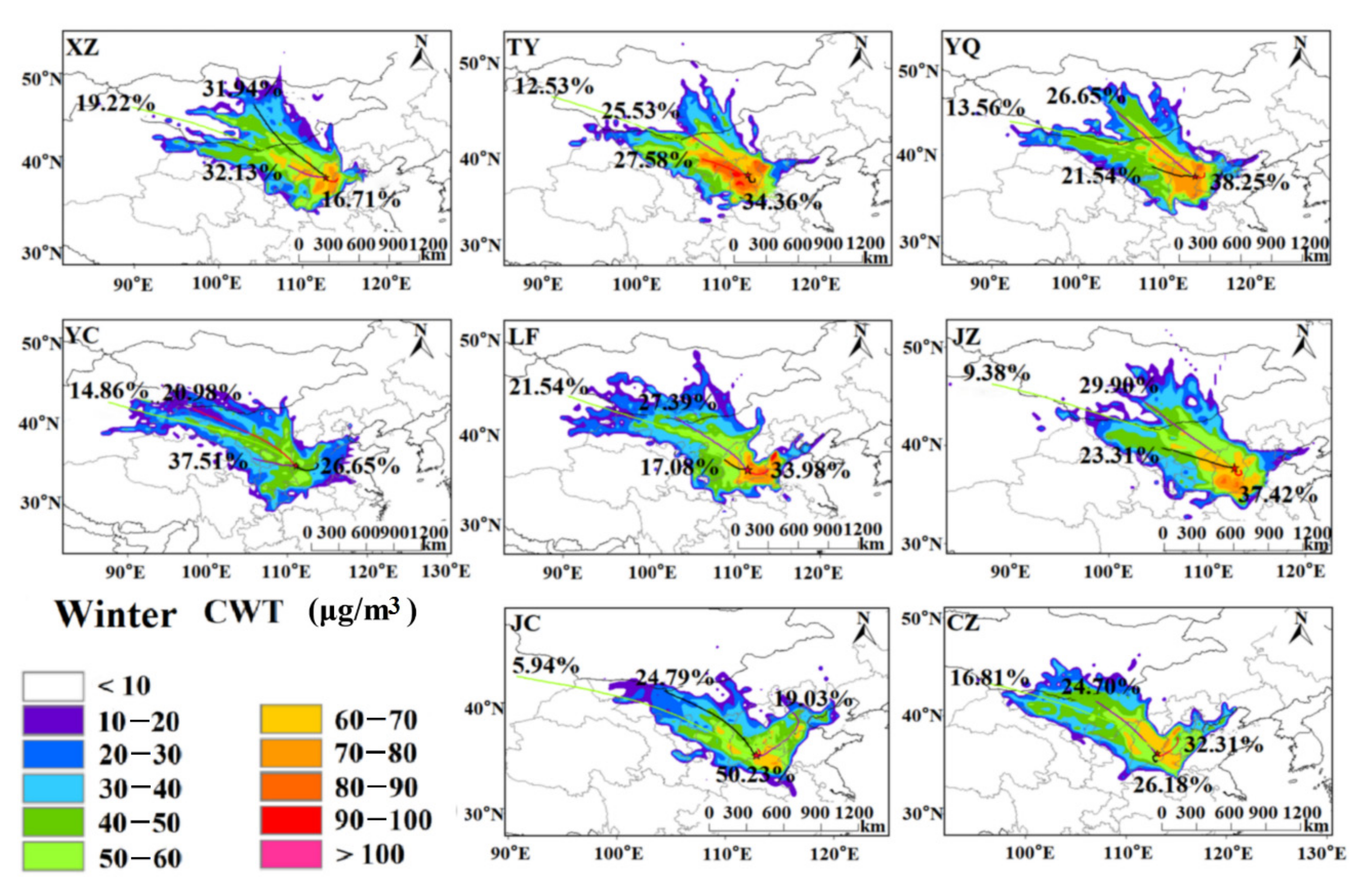
Figure 12.
CWT maps for NO2 by mass concentration (μg/m3) in winter in the cities having over-standard days.
In spring (Figure 9 and Figure S4), LL, YQ, JC, TY, LF and JZ were influenced by heavy input of NO2, while central-north Shaanxi and central-south Shanxi were identified by CWT as the main source areas. The areas around Erdos in Inner Mongolia, Yinchuan in Qinghai, northern Henan and south of Shijiazhuang in Hebei also contributed to the NO2 pollution of the above cities. The contribution of central-south Shanxi to NO2 reached above 100 μg/m3. Air masses from the areas around Huanghe River on the Shanxi-Shaanxi border had a certain contribution to NO2 in SZ and XZ.
In summer (Figure 10 and Figure S5), LL, TY, JC, YQ and JZ were influenced by heavy input of NO2. As in spring, central-north Shaanxi and central-south Shanxi were found to be the main source areas with central Shaanxi between Yan’an and Xi’an being the hotspot of CWT for LL, TY, YQ and JZ. YC was the the hotspot of CWT for JC. In addition, Northern Henan also had strong contribution to NO2 in JC and LL. The areas around Huhhot in Inner Mongolia were another potential source area for LL.
In autumn (Figure 11 and Figure S6), local Shanxi, especially the central and southern parts became the main source areas, followed by northern Henan and southern Hebei. The most affected cities included YQ, TY, JC, LL, JZ and XZ. The areas around Huhhot in Inner Mongolia were also the important source areas for some cities, such as YQ, TY and JZ.
In winter (Figure 12 and Figure S7), NO2 concentrations in TY, YQ, JZ, XZ, LF and CZ were influenced markedly by air masses incoming from their surrounding areas. The main source areas were within Shanxi, while the air masses originating from the adjacent regions in the surrounding provinces such as Henan, Hebei and Inner Mongolia also had some contributions. Northern Shaanxi had non-ignorable influence to the NO2 pollution in TY.
A seasonal comparison showed that NO2 concentrations in DT and CZ were influenced by regional transportation mainly in winter, while the influence in other seasons was very weak. For XZ, the influence of regional transportation was strong in winter and spring, while weak in summer and autumn. In LL, the influence of regional transportation was strongest in spring and summer followed by autumn, while weakest in winter. Summer had the similar potential source regions with spring, while winter had the similar source regions with autumn. For TY, both the influences of local emission and regional transportation were strong in all the seasons, but the potential source regions were different in different seasons. For YQ, the influence of regional transportation was strongest in spring, followed by autumn and winter, while weakest in summer. Local emissions also had large contributions. In YC, the regional transportation only had a certain influence on the NO2 concentration in spring, while the influence was very weak in other seasons. For LF, the influence of regional transportation was strongest in spring and winter, followed by autumn, while weakest in summer. The potential source regions were also different in different seasons like TY. JC was affected by regional transportation mainly in spring, summer, and autumn, while JZ was mainly in spring, autumn and winter.
4. Conclusions
Shanxi province is a hot spot of air pollution in China with the air quality of 4~5 cities are often in the bottom 20 of 168 major cities. To provide a basis for the formulation of future urban air pollution control measures to this province, the spatial-temporal distribution and variation of NO2 and its sources and chemical sinks were analyzed systematically in this study. Space-time differences were detected in each aspect.
- (1)
- The concentrations of NO2 in winter were significantly higher than that in other seasons due to the heating-related increase of combustion emissions in cold days, and thus the over-standard days were mainly concentrated in the heating season. The over-standard rate was the highest in TY (15.60%), followed by LF (9.86%), XZ (9.15%), JZ (8.45%) and YQ (7.75%).
- (2)
- Spacial distribution analysis showed that the areas with high NO2 pollution mainly concentrated in the central part of Shanxi Province from southwest to northeast (LL/LF–TY/JZ–YQ/JZ). Spatial autocorrelation analysis indicated that TY was the hot spot of NO2 pollution in winter, while LL was the hot spot in summer. Besides coal combustion, traffic exhaust is a key source need to be controlled stringently to alleviate NO2 pollution in TY. An integrated planning and a detailed technical scheme based on quantitatively source apportionment is necessary for the government of LL to promote an overall decline of NO2 concentration over the year as a whole, because its annual average exceeded the national standard required by GB3095-2012, but no day was over-standard.
- (3)
- Under the cooperative influence of anthropogenic activities, terrain and meteorological conditions, the cities displayed four types of monthly variation characteristics. Solar radiation and air temperature strongly impacted the daily variation of NO2 concentrations and its sink reactions forming O3 and PM2.5, resulting in different spatial distribution of NO2 concentration from O3 and PM2.5, as well as seasonal difference of the correlation between NO2 and PM2.5.
- (4)
- The correlation analysis between NO2 and other air pollutants implies that coal burning, traffic exhaust, coke production and non-coal-burning industries with high-temperature combustion of natural gas should be important sources of NO2 in Shanxi. The dominant sources were different in different cities.
- (5)
- The central-north Shaanxi, central-south Shanxi, northern Henan, south of Shijiazhuang and areas around Erdos in Inner Mongolia were important source areas influencing the pollution situation of NO2 in Shanxi. Therefore, joint air pollution control with these areas is critical to solve the air pollution problems in Shanxi.
Because only the concentrations of the six criteria pollutants are available in this study, it is hard to identify the source categories and clarify their contributions quantitatively with receptor models. The analysis of reaction sinks for NO2 to form PM2.5 and O3 was also just based on the correlation analysis. To have a clearer understanding about the sources of NO2 and the chemical reactions (including photochemical reactions) involved in the formation of secondary fine particles and O3, deeper model analysis is necessary in the future. However, the premise is that the monitoring networks could not only provide the data about the six criteria pollutants but also about the chemical constituents in PM2.5 and volatile organic compounds (VOCs) which are the critical precursors of PM2.5 and O3. That is, the function of the air pollution monitoring stations in China needs to be strengthened further.
Supplementary Materials
The following supporting information can be downloaded at: https://www.mdpi.com/article/10.3390/atmos13071096/s1, Figure S1: Annual wind speed chart of Lvliang City in 2018; Figure S2: The spatial distribution of the annual average concentrations of NO2, SO2, PM2.5 and O3 in Shanxi province; Figure S3: The monthly average concentrations of NO2, PM2.5 and O3 in different cities in the high-incidence months (June, July, August and September) of O3 pollution; Figure S4: CWT maps for NO2 by mass concentration (μg/m3) in spring in the cities without over-standard days; Figure S5: CWT maps for NO2 by mass concentration (μg/m3) in summer in the cities without over-standard days; Figure S6: CWT maps for NO2 by mass concentration (μg/m3) in autumn in the cities without over-standard days; Figure S7: CWT maps for NO2 by mass concentration (μg/m3) in winter in the cities without over-standard days; Table S1: Summary of meterological parameters in the prefectural cities in Shanxi.
Author Contributions
Conceptualization, H.L. (Hongyan Li); Formal Analysis, H.L. (Hongyan Li), J.Z., B.W., S.H., S.G. and Z.Z.; Investigation, B.W., J.Z., Z.Z. and G.F.; Resources, H.L. (Hongyan Li); Data Curation, H.L. (Hongyan Li), J.Z., B.W., Y.Z. and G.F.; Writing—Original Draft Preparation, H.L. (Hongyan Li); Writing—Review & Editing, H.L. (Hongyan Li), J.Z., B.W., S.H., H.L. (Hongyu Li), J.B., Y.C., Q.H. and Z.W.; Visualization, J.Z., S.H., S.G., Y.Z. and J.B.; Supervision, H.L. (Hongyan Li) and H.L. (Hongyu Li); Project Administration, H.L. (Hongyan Li); Funding Acquisition, H.L. (Hongyan Li). All authors have read and agreed to the published version of the manuscript.
Funding
This research was funded by the Shanxi Provincial Applied basic research program, China (201901D111250, 201901D111251); the Shanxi Provincial Key Research and Development Project (International Cooperation), China (201803D421095); the National Natural Science Foundation of China (22076135, 42077201).
Institutional Review Board Statement
Not applicable.
Informed Consent Statement
Not applicable.
Conflicts of Interest
The authors declare no conflict of interest.
Abbreviations
PM, Particulate Matter; CWT, Concentration Weighted Trajectory; O3, Ozone; APPCAP, Air Pollution Prevention and Control Action Plan; SO2, Sulfur Dioxide; NO2, Nitrogen Dioxide; RH, Relative Humidity; EU, European Union; WHO, World Health Organization; AQG, Air Quality Guidelines; YRD, Yangtze River Delta; CO, Carbon Monoxide; SCAS, State Controlling Air Sampling; CNEMC, China National Environmental Monitoring Center; GIS, Geography Information System; GMS, Globalization Modeling System; LISA, Local Indicator of Spatial Association; NAAQS, Chinese National Ambient Air Quality Standards.
References
- Li, K.; Jacob, D.J.; Liao, H.; Zhu, J.; Shah, V.; Shen, L.; Bates, K.H.; Zhang, Q.; Zhai, S.X. A two-pollutant strategy for improving ozone and particulate air quality in China. Nat. Geosci. 2019, 12, 906–910. [Google Scholar] [CrossRef]
- Maji, K.J. Substantial changes in PM2.5 pollution and corresponding premature deaths across China during 2015–2019: A model prospective. Sci. Total Environ. 2020, 729, 138838. [Google Scholar] [CrossRef] [PubMed]
- Jerrett, M.; Burnett, R.T.; Pope III, C.A.; Ito, K.; Thurston, G.; Krewski, D.; Shi, Y.; Calle, E.; Thun, M. Long-term ozone exposure and mortality. N. Engl. J. Med. 2009, 360, 1085–1095. [Google Scholar] [CrossRef] [Green Version]
- Turner, M.C.; Jerrett, M.; Pope III, C.A.; Krewski, D.; Gapstur, S.M.; Diver, W.R.; Beckerman, B.S.; Marshall, J.D.; Su, J.; Crouse, D.L. Long-term ozone exposure and mortality in a large prospective study. Am. J. Respir. Crit. Care Med. 2016, 193, 1134–1142. [Google Scholar] [CrossRef] [PubMed] [Green Version]
- Feng, Y.; Ning, M.; Lei, Y.; Sun, Y.; Liu, W.; Wang, J. Defending blue sky in China: Effectiveness of the “Air Pollution Prevention and Control Action Plan” on air quality improvements from 2013 to 2017. J Environ. Manage. 2019, 252, 109603. [Google Scholar] [CrossRef]
- Wang, G.; Zhang, R.; Gomez, M.E.; Yang, L.; Levy Zamora, M.; Hu, M.; Lin, Y.; Peng, J.; Guo, S.; Meng, J.; et al. Persistent sulfate formation from London Fog to Chinese haze. Proc. Natl. Acad. Sci. USA 2016, 113, 13630–13635. [Google Scholar] [CrossRef] [PubMed] [Green Version]
- Xie, Y.; Wang, G.; Wang, X.; Chen, J.; Chen, Y.; Tang, G.; Wang, L.; Ge, S.; Xue, G.; Wang, Y. Nitrate-dominated PM2.5 and elevation of particle pH observed in urban Beijing during the winter of 2017. Atmos. Chem. Phys. 2020, 20, 5019–5033. [Google Scholar] [CrossRef]
- Agudelo-Castañeda, D.; De Paoli, F.; Morgado-Gamero, W.B.; Mendoza, M.; Parody, A.; Maturana, A.Y.; Teixeira, E.C. Assessment of the NO2 distribution and relationship with traffic load in the Caribbean coastal city. Sci. Total Environ. 2020, 720, 137675. [Google Scholar] [CrossRef]
- Xue, R.; Wang, S.; Li, D.; Zou, Z.; Chan, K.L.; Valks, P.; Saiz-Lopez, A.; Zhou, B. Spatio-temporal variations in NO2 and SO2 over Shanghai and Chongming Eco-Island measured by Ozone Monitoring Instrument (OMI) during 2008–2017. J. Clean Prod. 2020, 258, 120563. [Google Scholar] [CrossRef]
- Krotkov, N.A.; McLinden, C.A.; Li, C.; Lamsal, L.N.; Celarier, E.A.; Marchenko, S.V.; Swartz, W.H.; Bucsela, E.J.; Joiner, J.; Duncan, B.N.; et al. Aura OMI observations of regional SO2 and NO2 pollution changes from 2005 to 2015. Atmos. Chem. Phys. 2016, 16, 4605–4629. [Google Scholar] [CrossRef] [Green Version]
- Wang, C.; Wang, T.; Wang, P.; Wang, W. Assessment of the Performance of TROPOMI NO2 and SO2 Data Products in the North China Plain: Comparison, Correction and Application. Remote Sens. 2022, 14, 214. [Google Scholar] [CrossRef]
- Mak, H.; Laughner, J.; Fung, J.; Zhu, Q.; Cohen, R. Improved Satellite Retrieval of Tropospheric NO2 Column Density via Updating of Air Mass Factor (AMF): Case Study of Southern China. Remote Sens. 2018, 10, 1789. [Google Scholar] [CrossRef] [Green Version]
- Xu, J.; Lindqvist, H.; Liu, Q.; Wang, K.; Wang, L. Estimating the spatial and temporal variability of the ground-level NO2 concentration in China during 2005–2019 based on satellite remote sensing. Atmos. Pollut. Res. 2021, 12, 57–67. [Google Scholar] [CrossRef]
- Zhao, H.; Chen, K.; Liu, Z.; Zhang, Y.; Shao, T.; Zhang, H. Coordinated control of PM2.5 and O3 is urgently needed in China after implementation of the “Air pollution prevention and control action plan”. Chemosphere 2021, 270, 129441. [Google Scholar] [CrossRef] [PubMed]
- Lin, Y.C.; Zhang, Y.L.; Fan, M.Y.; Bao, M.Y. Heterogeneous formation of particulate nitrate under ammonium-rich regimes during the high-PM2.5 events in Nanjing, China. Atmos. Chem. Phys. 2020, 20, 3999–4011. [Google Scholar] [CrossRef] [Green Version]
- Wang, W.C.; Chang, Y.J.; Wang, H.C. An Application of the Spatial Autocorrelation Method on the Change of Real Estate Prices in Taitung City. ISPRS Int. J. Geo-Inf. 2019, 8, 249. [Google Scholar] [CrossRef] [Green Version]
- Wen, L.; Chen, J.; Yang, L.; Wang, X.; Xu, C.; Sui, X.; Yao, L.; Zhu, Y.; Zhang, J.; Zhu, T. Enhanced formation of fine particulate nitrate at a rural site on the North China Plain in summer: The important roles of ammonia and ozone. Atmos. Environ. 2015, 101, 294–302. [Google Scholar] [CrossRef]
- Zou, J.; Liu, Z.; Hu, B.; Huang, X.; Wen, T.; Ji, D.; Liu, J.; Yang, Y.; Yao, Q.; Wang, Y. Aerosol chemical compositions in the North China Plain and the impact on the visibility in Beijing and Tianjin. Atmos. Res. 2018, 201, 235–246. [Google Scholar] [CrossRef]
- Zhao, S.; Yu, Y.; Yin, D.; He, J.; Liu, N.; Qu, J.; Xiao, J. Annual and diurnal variations of gaseous and particulate pollutants in 31 provincial capital cities based on in situ air quality monitoring data from China National Environmental Monitoring Center. Environ. Int. 2016, 86, 92–106. [Google Scholar] [CrossRef]
- Tian, D.; Fan, J.; Jin, H.; Mao, H.; Geng, D.; Hou, S.; Zhang, P.; Zhang, Y. Characteristic and Spatiotemporal Variation of Air Pollution in Northern China Based on Correlation Analysis and Clustering Analysis of Five Air Pollutants. J. Geophys. Res. Atmos. 2020, 125, e2019JD031931. [Google Scholar] [CrossRef]
- Chu, B.; Ma, Q.; Liu, J.; Ma, J.; Zhang, P.; Chen, T.; Feng, Q.; Wang, C.; Yang, N.; Ma, H. Air Pollutant Correlations in China: Secondary Air Pollutant Responses to NOx and SO2 Control. Environ. Sci. Technol. Lett. 2020, 7, 695–700. [Google Scholar] [CrossRef]
- Li, J.; Li, H.; He, Q.; Guo, L.; Zhang, H.; Yang, G.; Wang, Y.; Chai, F. Characteristics, sources and regional inter-transport of ambient volatile organic compounds in a city located downwind of several large coke production bases in China. Atmos. Environ. 2020, 233, 117573. [Google Scholar] [CrossRef]
- Bulletin of Eco Environmental Status of Shanxi in 2018. Available online: https://sthjt.shanxi.gov.cn/xwzx_1/hjyw/202111/t20211114_3241339.shtml (accessed on 5 November 2021).
- Wang, Z.; Lv, J.; Tan, Y.; Guo, M.; Gu, Y.; Xu, S.; Zhou, Y. Temporospatial variations and Spearman correlation analysis of ozone concentrations to nitrogen dioxide, sulfur dioxide, particulate matters and carbon monoxide in ambient air, China. Atmos. Pollut. Res. 2019, 10, 1203–1210. [Google Scholar] [CrossRef]
- Zhai, S.; Jacob, D.J.; Wang, X.; Shen, L.; Li, K.; Zhang, Y.; Gui, K.; Zhao, T.; Liao, H. Fine particulate matter (PM2.5) trends in China, 2013–2018: Separating contributions from anthropogenic emissions and meteorology. Atmos. Chem. Phys. 2019, 19, 11031–11041. [Google Scholar] [CrossRef] [Green Version]
- Shanxi Statistical Yearbook—2018. Available online: http://tjj.shanxi.gov.cn/tjsj/tjnj/nj2018/indexch.htm (accessed on 8 November 2021).
- Zhang, L.; Qiao, L.; Lan, J.; Yan, Y.; Wang, L. Three-years monitoring of PM2.5 and scattering coefficients in Shanghai, China. Chemosphere 2020, 253, 126613. [Google Scholar] [CrossRef] [PubMed]
- Hu, J.; Ying, Q.; Wang, Y.; Zhang, H. Characterizing multi-pollutant air pollution in China: Comparison of three air quality indices. Environ. Int. 2015, 84, 17–25. [Google Scholar] [CrossRef]
- Lu, X.; Hong, J.; Zhang, L.; Cooper, O.R.; Schultz, M.G.; Xu, X.; Wang, T.; Gao, M.; Zhao, Y.; Zhang, Y. Severe surface ozone pollution in China: A global perspective. Environ. Sci. Technol. Lett. 2018, 5, 487–494. [Google Scholar] [CrossRef]
- Ambient air—Automatic Determination of Nitrogen Oxides—Chemiluminescence Method (HJ 1043-2019). Available online: https://www.mee.gov.cn/ywgz/fgbz/bz/bzwb/jcffbz/201911/W020191104352508999799.pdf (accessed on 5 March 2021).
- Technical Guideline on Environmental Monitoring Quality Management. Available online: https://www.mee.gov.cn/ywgz/fgbz/bz/bzwb/other/qt/201109/W020120130585014685198.pdf (accessed on 8 March 2021).
- Ambient Air Quality Standards (GB 3095-2012). Available online: http://www.cnemc.cn/jcgf/dqhj/201711/P020181010540074249753.pdf (accessed on 5 March 2021).
- Griffith, D.A.; Paelinck, J.H. Morphisms for Quantitative Spatial Analysis; Springer: Berlin/Heidelberg, Germany, 2018. [Google Scholar]
- Sowunmi, F.; Akinyosoye, V.; Okoruwa, V.; Omonona, B. The Landscape of Poverty in Nigeria: A Spatial Analysis Using Senatorial Districts-level Data. Am. J. Econ. 2012, 2, 61–74. [Google Scholar]
- Wubuli, A.; Xue, F.; Jiang, D.; Yao, X.; Upur, H.; Wushouer, Q. Socio-demographic predictors and distribution of pulmonary tuberculosis (TB) in Xinjiang, China: A spatial analysis. PLoS ONE 2015, 10, e0144010. [Google Scholar] [CrossRef]
- Guilmoto, C.Z. Spatial regression and determinants of juvenile sex ratio in India. In Proceedings of the International Conference on Female Deficit in Asia: Trends and Perspectives, Singapore, 5–7 December 2005. [Google Scholar]
- Zhang, L.; Wang, H.; Song, Y.; Wen, H. Spatial spillover of house prices: An empirical study of the Yangtze Delta urban agglomeration in China. Sustainability 2019, 11, 544. [Google Scholar] [CrossRef] [Green Version]
- Bivand, R.; Altman, M.; Anselin, L.; Assunção, R. Spatial Dependence: Weighting Schemes, Statistics and Models. R package. Available online: http://CRAN.R-project.org/package=spdep (accessed on 10 March 2021).
- Wang, Y.; Zhang, X.; Draxler, R.R. TrajStat: GIS-based software that uses various trajectory statistical analysis methods to identify potential sources from long-term air pollution measurement data. Environ. Modell. Softw. 2009, 24, 938–939. [Google Scholar] [CrossRef]
- Wang, Y.; Zhang, X.; Arimoto, R. The contribution from distant dust sources to the atmospheric particulate matter loadings at XiAn, China during spring. Sci. Total Environ. 2006, 368, 875–883. [Google Scholar] [CrossRef] [PubMed]
- Squizzato, S.; Masiol, M. Application of meteorology-based methods to determine local and external contributions to particulate matter pollution: A case study in Venice (Italy). Atmos. Environ. 2015, 119, 69–81. [Google Scholar] [CrossRef]
- Fan, W.; Qin, K.; Xu, J.; Yuan, L.; Li, D.; Jin, Z.; Zhang, K. Aerosol vertical distribution and sources estimation at a site of the Yangtze River Delta region of China. Atmos. Res. 2019, 217, 128–136. [Google Scholar] [CrossRef] [Green Version]
- Zachary, M. Application of PSCF and CWT to Identify Potential Sources of Aerosol Optical Depth in ICIPE Mbita. Open Access Library J. 2018, 5, 1. [Google Scholar] [CrossRef]
- Shen, F.; Zhang, L.; Jiang, L.; Tang, M.; Gai, X.; Chen, M.; Ge, X. Temporal variations of six ambient criteria air pollutants from 2015 to 2018, their spatial distributions, health risks and relationships with socioeconomic factors during 2018 in China. Environ. Int. 2020, 137, 105556. [Google Scholar] [CrossRef]
- Stockwell, W.R.; Lawson, C.V.; Saunders, E.; Goliff, W.S. A review of tropospheric atmospheric chemistry and gas-phase chemical mechanisms for air quality modeling. Atmosphere 2011, 3, 1–32. [Google Scholar] [CrossRef] [Green Version]
- Anselin, L.; Sridharan, S.; Gholston, S. Using exploratory spatial data analysis to leverage social indicator databases: The discovery of interesting patterns. Soc. Indic. Res. 2007, 82, 287–309. [Google Scholar] [CrossRef]
- Air Pollution Prevention and Control Action Plan. Available online: http://www.gov.cn/zwgk/2013-09/12/content2486773.htm (accessed on 5 November 2018).
- Wang, Y.; Cheng, K.; Tian, H.-Z.; Yi, P.; Xue, Z.-G. Analysis of Reduction Potential of Primary Air Pollutant Emissions from Coking Industry in China. Aerosol Air Qual. Res. 2018, 18, 533–541. [Google Scholar] [CrossRef]
- Zhong, Q.; Shen, H.; Yun, X.; Chen, Y.; Ren, Y.; Xu, H.; Shen, G.; Du, W.; Meng, J.; Li, W.; et al. Global Sulfur Dioxide Emissions and the Driving Forces. Environ. Sci. Technol. 2020, 54, 6508–6517. [Google Scholar] [CrossRef]
- Wang, S.X.; Zhao, B.; Cai, S.Y.; Klimont, Z.; Nielsen, C.P.; Morikawa, T.; Woo, J.H.; Kim, Y.; Fu, X.; Xu, J.Y.; et al. Emission trends and mitigation options for air pollutants in East Asia. Atmos. Chem. Phys. 2014, 14, 6571–6603. [Google Scholar] [CrossRef] [Green Version]
- Li, H.; Guo, L.; Cao, R.; Gao, B.; Yan, Y.; He, Q. A wintertime study of PM2.5-bound polycyclic aromatic hydrocarbons in Taiyuan during 2009–2013: Assessment of pollution control strategy in a typical basin region. Atmos. Environ. 2016, 140, 404–414. [Google Scholar] [CrossRef]


Publisher’s Note: MDPI stays neutral with regard to jurisdictional claims in published maps and institutional affiliations. |
© 2022 by the authors. Licensee MDPI, Basel, Switzerland. This article is an open access article distributed under the terms and conditions of the Creative Commons Attribution (CC BY) license (https://creativecommons.org/licenses/by/4.0/).