Abstract
One of the main problems faced by the Belém Metropolitan Region (BMR) inhabitants is flash floods caused by precarious infrastructure and extreme rainfall events. The objective of this article is to investigate whether and how the local urban characteristics may influence the development of thunderstorms. The Weather Research and Forecasting (WRF) model was used with three distinct configurations of land use/cover to represent urbanization scenarios in 2017 and 1986 and the forest-only scenario. The WRF model simulated reasonably well the event. The results showed that the urban characteristics of the BMR may have an impact on storm systems in the urban areas close to the Northern Coast of South America. In particular, for the urban characteristics in the BMR in 2017, the intensification of the storm may be linked to a higher value of energy available for convection (over 1000 J kg−1) and favorable wind convergence and vertical shear in the urban area (where the wind speed at the surface was more than 3 m s−1 slower than in the forest-only scenario). Meanwhile, the other land cover scenarios could not produce a similar storm due to lack of moisture, wind convergence/shear, or convective energy.
1. Introduction
The climate inside a city is not the same as in its neighboring areas and must not be considered the same as its surroundings [1]. The materials, structures, and shapes of cities change the urban-free atmospheric conditions, creating what is called “urban climate”. The differences can be observed in many meteorological variables due to the influence of materials, such as concrete and asphalt that can store and emit more heat back to the atmosphere. Thus, the air temperature is expected to be higher in cities than in rural regions, defining the so-called urban heat island (UHI) [2,3]; the lack of vegetation and higher surface runoff weakens the hydrological cycle reducing atmospheric moisture. The wind speed is reduced as a consequence of the enhanced surface roughness caused by buildings that prevent the circulation of moisture and heat [4,5,6,7,8]. With all these changes to the lower atmosphere, the cities will also influence the development and movement of storms that enter the urban area.
The city’s UHI can intensify (or even initiate) storms that enter the city domain by enhancing the convection. Increased heat and consequently convective available potential energy (CAPE) due to urbanization have been associated with increased thunderstorm activity over India [9,10], Brazil [11], the United States [12], and China [13]. However, heat is not the only factor to be considered, and depending on the regional wind velocity, this process can happen up- or downwind [14,15,16].
Similar to the UHI, city buildings can have two distinct effects: the enhanced roughness length (caused by the building’s height) increases the convergence at the surface and generates turbulence that destabilizes the atmosphere, favoring the development of stronger storms [2,17,18], but the buildings can also serve as barriers to the wind flow diverting the storm from the city by either splitting it or blocking its path [17,18,19]. Aerosols also have an important role in storm development by changing cloud properties and dynamics, such as the updraft and downdraft timing, precipitation amount, and droplet size [20]. Even though cities can produce a significant amount of aerosols, this information was not considered in this study, since the study area does not have any observed information regarding it.
In the Brazilian part of the Amazon Rain Forest, one of the most important urban areas is located at its northeastern border, and it is called Belém Metropolitan Region (BMR). This area is formed by seven municipalities that are brought together by its socio-economical characteristics. From these seven municipalities, Belém, Ananindeua, and Marituba are the municipalities where most of the BMR population, businesses, and industry are located [21]; therefore, in this study, the acronym BMR stands for these three places.
One of the main sources of vulnerability for its population is the risk of floods, often associated with extreme precipitation events, but far from it being the only reason for flooding [22]. Previous studies have pointed out that the BMR region has a favorable condition for the development of deep convective systems that can produce large values of accumulated precipitation (mostly due to the high CAPE observed in the region and wind dynamics) and that extreme precipitation events are becoming more frequent [23,24,25].
Besides, reference [26] showed that part of Belém’s inhabitants is perceiving changes in the city’s climate. According to their survey, Belém is getting warmer and drier, with a higher variability of the precipitation events intensity. This information was corroborated by analyzing data from the Brazilian National Institute of Meteorology (INMET) from 1980 to 2018. The authors concluded that, although the temperature and moisture changes may be associated with a global climate change process (or even a regional process due to Eastern Amazon deforestation [27,28]), the precipitation variability may also be linked with the local development of the urban area.
However, even though those studies have shown evidence regarding the urban effect on precipitation, there has not been one research that tried to simulate it and fully analyze the surface−atmosphere interaction. As mentioned before, the BMR is one of the most important and largest areas in Northern Brazil, and its population is beginning to notice the effects of local climate change. It is necessary to study how the landscape is contributing to this climate change process, so its population can be prepared for future scenarios.
Thus, the purpose of this paper is to investigate the influence of the Belém urban area on the development of a thunderstorm that happened on 7 June 2011 using the Weather Research and Forecasting (WRF) model with different land use/cover scenarios.
2. Materials and Methods
2.1. Study Area
The BMR is located in the Eastern Amazon, approximately 125 km on a straight line from the Atlantic Ocean, and the climate is tropical humid, with an average temperature between 25.4 and 26.5 °C and an average accumulated annual precipitation of 2800 mm year−1, according to the Belém’s meteorological station of the INMET [29]).
As a baseline for the comparison between the reality and how the region is represented by the model land use/cover data, Figure 1 shows a natural-colored image of the BMR from Landsat 8. Figure 2 shows the domain used by the WRF model and how the urban scenarios were defined: (a) the entire model domain (Figure 2a); (b) the default urban settings from the WRF (land use from MODIS; Figure 2b); (c) urbanization in 1986 (Figure 2c; the oldest satellite image found for the BMR without cloud interference); (d) urbanization in 2017 (Figure 2d). In addition, a forest-only scenario was created (not shown) where all urban tiles were replaced by an evergreen forest. It is important to note that all these land use/cover included the BMR.
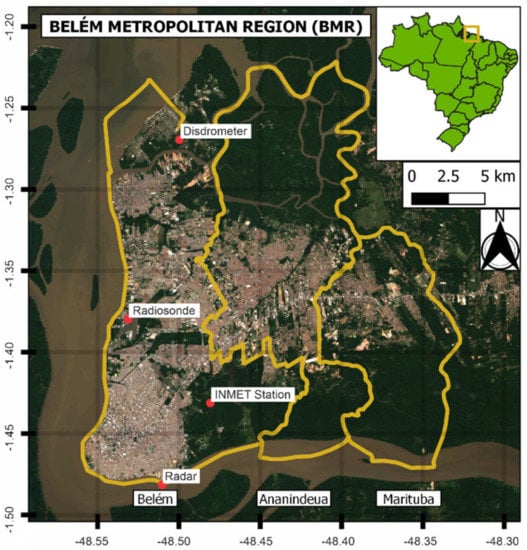
Figure 1.
Satellite image from Landsat 8 of the Belém Metropolitan Region (BMR) focused on the main urbanized area of Belém, Ananindeua, and Marituba (yellow contour). The red dots mark the location of the instruments used: Radiosonde (−1.38° and −48.48°), the INMET surface station (−1.43° and −48.43°), the Radar (−1.48° and −48.46°) and Chuja Project Disdrometer (−1.27° and −48.46°).
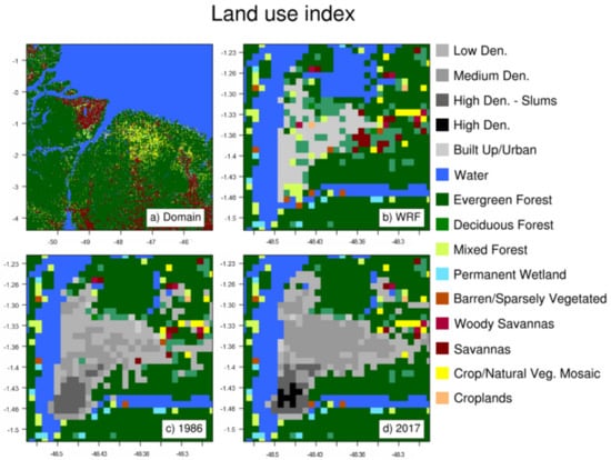
Figure 2.
Weather Research and Forecasting (WRF) land use categories. (a) entire domain; (b) WRF default categories; (c) BMR urban area as in 1986; (d) BMR area as in 2017. The solid black lines represent the real geography of the area.
The BRM is not well represented by the model (Figure 2b), and to improve its representation, the amount of impervious land was extracted from Landsat 5 (1986) and Landsat 8 (2017) satellite images according to the impervious built-up index (IBI) calculation. The main difference observed between each year was the reduction of forest cover and the expansion of the urban area, with a higher density urban area appearing in the middle of what is considered the center of Belém (to the south, around 1.4° S and 48.52° W), and especially the expansion of the medium-density category (both categories were described below). The BMR is dominated by urban and forest land cover and areas destinated to crop growth are small in size and often are hidden by trees, so they are very difficult to be classified by satellite imagery.
Proposed by Xu [30] and discussed by Sekertekin et al. [31], the IBI can produce a better classification of urban features due to its composition of three thematic indices: soil-adjusted vegetation index (SAVI), normalized difference build-up index (NDBI), and modified normalized difference water index (MNDWI). These three indices were selected to represent the complexity of the urban ecosystem and were used as “bands” for the IBI calculation following Equation (1):
The IBI ranges from 0 (no impervious surface) to 1 (completely impervious surface), and as defined by the authors, each of the three main classes (low, medium, and high densities; the latter was divided into two categories described below) received a third of this range. Each urban category for the 2017 scenario was defined based on the IBI and according to the population density and the average household income information collected during the 2010 Census performed by the Brazilian Geography and Statistics Institute (IBGE). In 1986, the BMR was very different, especially in the outskirts where there were fewer buildings and more vegetation, so the 1986 scenario used almost the same categories, but with some changes as described below. Physical characteristics necessary for the model, such as emissivity, albedo, and roughness length, were from Souza [32]. The four categories are as following:
Low density: well-vegetated (70% natural vegetation), low buildings (5 ± 1 m), and impervious surface (between 0 and 0.3);
Medium density: some vegetation (30% natural vegetation), low–medium-height buildings (10 ± 3 m), and impervious surface between 0.3 and 0.7;
High-density slums: almost no vegetation (10% natural vegetation), low-height buildings (7.5 m ± 1 m), and impervious surface between 0.8 and 1. This category slightly changed for the 1986 scenario, with higher buildings (20 ± 10 m) and more vegetation (25% natural vegetation);
High density: almost no vegetation (10% natural vegetation), medium–tall building (60 ± 25 m), and impervious surface between 0.7 and 0.8. It was not present for the 1986 scenario.
2.2. Case Study and Model Configuration
The Chuva Project campaign happened in the BMR in June 2011. For the duration of the campaign, different new instruments were installed to monitor its atmosphere and the meteorological systems that moved over it [33].
Figure 3 is composed of infrared satellite images detailing the evolution of a meteorological system that happened on 7 June 2011 (the blue arrows indicate its position). The system began its development in the Atlantic Ocean late in the morning, reaching the continent between Pará and Maranhão states borders at 1600 UTC (the local time is UTC−3 h) (Figure 3a). As the system moved westward, it grew, and the top of the clouds got colder, indicating deeper clouds (Figure 3b). When it reached the BMR (Figure 3c; around 2000 UTC), the system reached its maximum development, with the minimum cloud top temperatures between −80 and −70 °C. The dissipation phase started just after it passed the BMR (Figure 3d; 2100 UTC) and reached Marajó Island (red arrow).
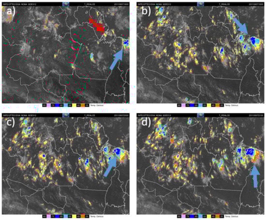
Figure 3.
Infrared satellite images from GOES 12 focused on the northern region of Brazil at 1600 UTC (a), 1930 UTC (b), 2000 UTC (c), and 2100 UTC (d). The colors represent the cloud top temperature, from −80 °C (pink) to −30 °C (orange). The blue arrows indicate the system of interest, and the red indicates where Marajó Island is located.
The INMET meteorological station (south of Belém, −1.43° and −48.43°) registered 38 mm of precipitation during the system passage over Belém, while the Chuva Project disdrometer (north of Belém) registered 27 mm of precipitation. Even though the accumulated precipitations in these sites were not extreme, the local media reported many problems related to the storm, such as traffic jams, floods, power shortages, and building damages. In conclusion, this event was well documented and caused many problems for the city, making it an ideal case study.
Different physics and dynamic combinations were tested to see how they simulated the selected event. A different source of initial condition was also evaluated. The options described below produced the best results for the control run.
The following settings were used for all three land use/cover scenarios described in Section 2.1. The model used for this experiment was version 3.8 of the WRF model [34]. The model simulated one grid of 600 × 600 points (Figure 2a), at a 1 km resolution, approximately with a time-step of 5 s and an output every 30 min. The initial and boundary conditions (updated every 6 h) were from the Global Forecast System [35]), and a constant sea surface temperature (SST) from the multi-scale ultra-high resolution (MUR–SST; [36]) dataset was also used. The WRF data assimilation system (WRFDA; [37]) was used to assimilate observational data from the Chuva Project radiosonde (from 1800 UTC of 6 June to 0000 UTC of 8 June and with 4 h intervals between each launch; with a total of 8 soundings records) and surface stations from the INMET (−1.43° and −48.43°) into the WRF first guess data.
The parameterizations used were as following: microphysics, Ferrier/ETA [38]; radiation, rapid radiative transfer model (RRTM) [39,40]; Monin–Obukhov surface scheme [41]; Mellor–Yamada–Janjic planetary boundary layer scheme [42]; Noah land surface model [43]. The urban effect was simulated using the building effect parametrization (BEP), a multilayer urban canopy model that places the buildings inside the lowest model layers, allowing the model to perform explicit interactions between the building and the atmosphere [44].
The model was integrated at three different times: 30 h (starting on 6 June 2011 at 1800 UTC), 24 h (starting on 7 June 2011 at 0000 UTC), and 18 h (starting on 7 June 2011 at 0600 UTC). These three different integration times changed how the storm was simulated (an example is presented in Figure S1 in Supplementary Materials) and the shorter time did not reproduce the event, while a longer integration time ended the simulation abruptly. The ensemble mean from these three integration times was calculated, and all results presented here are ensemble mean values. Additionally, all variables presented were estimated by the model or calculated using NCAR Command Language (NCL; in the case of CAPE, described in Equation (2)), except the Bulk Richardson Number that was calculated with Equation (3):
where EL is the height equilibrium level, LFC is the level of free convection, g is the gravity acceleration, Tv,env is the environment virtual temperature, Tv,parcel is the parcel virtual temperature, z is the height above ground, θV is the virtual potential temperature at z, θVS is the virtual potential temperature near the surface, and U(z) and V(z) are the horizontal wind components at z [45]. For this research, RiB was calculated for the layer between the surface and the height of 6000 m.
Considering that the objective of this research is the BMR’s influence on the storm and not how the system was generated and its lifespan, we did not investigate the reasons behind each test result.
3. Results and Discussion
3.1. Model Evaluation
The control run results of the WRF model (2017 scenario ensemble mean) was compared to radiosonde and radar observations. The model performed reasonably well for both data sets. At the ground level (Figure 4), although there were quantitative differences between the 2017 scenario and the observed, both had similar trends before and after the storm. The precipitation simulated by the model at the INMET station (−1.43° and −48.43°) had a one-hour lag, being closer to the disdrometer measure. Meanwhile, the equivalent potential temperature (EPT) was lower in the model run before the storm, indicating that the model’s atmosphere was drier and colder than the observed, but the difference was significantly reduced after the storm, as the air was transported from aloft to the surface and the atmosphere stabilized [46]. The wind speed decreased constantly in the model and the observed, maintaining an almost constant difference between them.
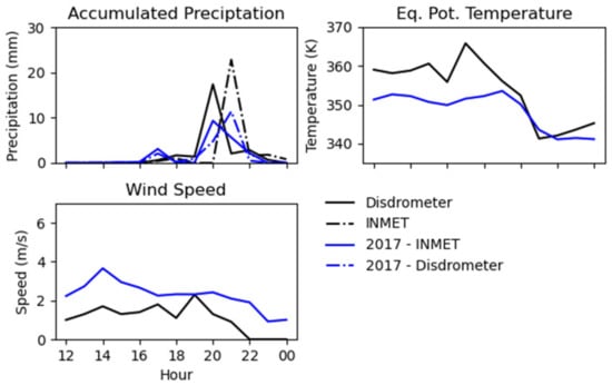
Figure 4.
Time series of the accumulated precipitation (mm h−1), the equivalent potential temperature (K), and the wind speed (m s−1) for the observed at the Brazilian National Institute of Meteorology (INMET) Station (black solid lines) and at the disdrometer (black dashed line) and the 2017 scenario at the INMET Station point (blue solid line) and at the disdrometer (blue dashed line).
The vertical profiles of the EPT and the wind speed of the model followed the observation trends, although quantitative differences were noted (Figure 5). In general terms, the model was colder and drier than the observation, but both of them displayed an unstable layer of the atmosphere near the surface since the temperature decreased with the height.
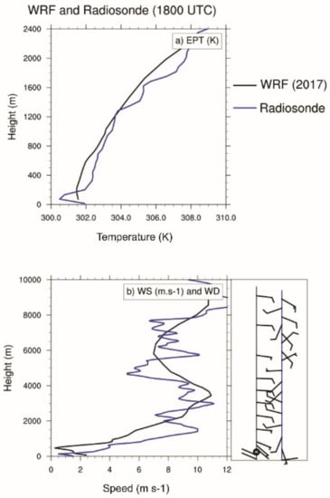
Figure 5.
WRF (black) and radiosonde (blue) vertical profiles at 1800 UTC of the equivalent potential temperature (K) (a) and the wind speed (WS) and direction (WD) (b).
The wind speed alternated between a positive and a negative bias. The model simulated easterly winds almost for the entire atmosphere, and only near the surface the wind had a northwesterly direction. The observation also showed westerly winds, but on higher layers and a southerly contribution. Easterly winds were noted at the surface and above 5 km.
The model and the radar reflectivity analysis (Figure 6) showed that the WRF model did not represent the correct orientation of the system, but the timing and direction of movement were adequately simulated. At 2000 UTC, the system presented a latitudinal orientation, with different storm cells throughout its extension. At the same time, the WRF model simulated a diagonal (from southwest to northeast) line with small storms and the main one near Belem, almost in the same position as the one seen by the radar. The leading storms, located to the southwest of the BMR, were also simulated, even though in a more localized manner.
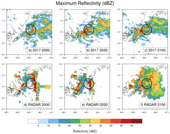
Figure 6.
WRF (a–c) and radar (d–f) maximum reflectivities observed through the entire model height (dBZ) for three periods: 2000 (a,d), 2030 (b,e), and 2100 UTC (c,f) on 7 June 2011. The black circle marks the BMR location.
At 2030 UTC, the system was concentrated over the BMR, and the model also simulated the storm in the same position but kept the diagonal orientation. An intense convective region, above 40 dBZ, extended to the southwest, while the radar observed a similar structure but positioned directly south of the BMR.
After the system passed the BMR, it broke into small storms to the west and over the river, and in the WRF simulation, a similar process was noted. The main difference was found in the rear of the storm, as the only region with active convective movement in the model was to the northeast of the BMR. The radar showed a more active area all around the area of interest, with reflective of 35 dBZ or higher.
The noticed difference between the observed and modeled can be attributed to the small number of instruments available at the time to measure the atmospheric conditions to be used as initial conditions for the model [47]. Even so, the model performed reasonably well, reaching a maximum, at the BMR, above 40 dBZ at 2030 UTC, similar to the observed. At the next moment, this value was reduced to below 35 dBZ, higher than the radar, which was between 25 and 30 dBZ.
Another important parameter is the balance between wind shear and buoyance known as the Richardson Number (presented here as its bulk version). The RiB calculated at 1800 UTC (the last radiosonde launch before the storm) for the control run (at the radiosonde site) was 57 and 55 for the radiosonde. Weisman and Klemp [48] concluded that this value represents a good balance between both effects, ideal for multicell systems (like long-lasting squall lines, as observed by the radar) and non-tornadic supercell, which may be the case for the cell located above the BMR. Despite the differences, the model and observed atmosphere during the system lifetime were similar, reassuring that the storm over the BMR was reasonably well simulated.
3.2. WRF Sensitivity Analysis
Analyzing the time series from all scenarios and comparing them with the observed (Figure 7), it can be noticed that the 1986 and forest scenarios behaved similar to the 2017 one, as expected, since the location of the station has not changed its land cover, but the surrounding area has changed and its characteristics can be transported to the station site. In the case of the forest scenario, the higher moisture content in the atmosphere, which originated from the evapotranspiration process of the vegetation, elevated the EPT, while the lower roughness of the surface resulted in a higher wind speed. There were no significant differences between the urban scenarios, at least not in this location.
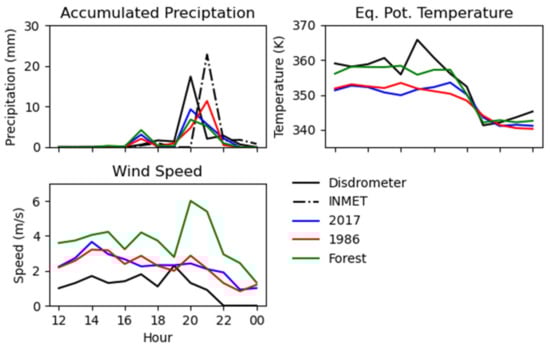
Figure 7.
Time series of the accumulated precipitation (mm h−1), the equivalent potential temperature (K), and the wind Speed (m s−1) for the observed at the INMET Station (black solid lines, located at −1.43° and −48.43°) and at the disdrometer (black dashed line, located at −1.27° and −48.45°) and the 2017 scenario at the INMET Station point (blue solid line) and at the disdrometer (blue dashed line).
The spatial distribution of the accumulated precipitation during the storm between 1930 and 2100 UTC are shown (Figure 8). In all scenarios, part of the storm followed the river to the south of the BMR. However, there was less precipitation in the middle of the study area in the year 1986 scenario than in the forest one and especially in the year 2017 scenario, which displayed a large area in the middle of the BMR with a significant amount of precipitation during the storm.
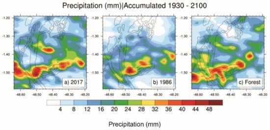
Figure 8.
Total accumulated precipitations between 1930 and 2100 UTC.
Maximum reflectivity (dBZ) was detected on the entire model height, and it is presented in Figure 9 for all scenarios. Before the system arrived at 1930 UTC, all scenarios displayed a similar reflectivity, with more clouds at the center and to the north of the town. At 2000 UTC, a large region with a reflectivity higher than 35 dBZ can be noticed in the 2017 scenario, but not in the 1986 scenario and over a smaller region in the forest one. Almost the entire BMR domain had a reflectivity higher than 35 dBZ at 2030 UTC during the 2017 scenarios, especially in the middle of the BMR and on the southern river shore. Similar to what was noticed at 2000 UTC, the forest scenario resembled the 2017 scenario again, although the higher reflectivity was more concentrated in three places: northwest, middle, and southwest areas of the BMR. The ensemble mean of the 1986 scenario differed from the others, as the main areas with high reflectivity were to the west and south, outside the urban area. After the system passed over the BMR (2100 UTC), some regions with more than 35 dBZ can still be noted in 1986 and 2017, while lower values of dBZ were estimated by the forest scenario ensemble mean.
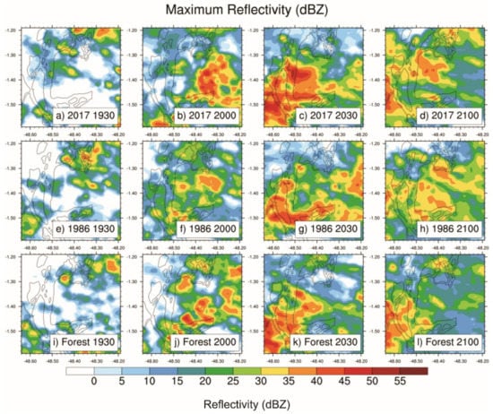
Figure 9.
Maximum reflectivities (dBZ) for the 2017 (a–d), 1986 (e–h), and forest (i–l) scenarios at 1930, 2000, 2030, and 2100 UTC.
Therefore, the ensemble means indicated that cloud formation was intensified in the 2017 scenario, indicating that urban centers have important characteristics that may influence the local atmosphere and alter storms in different ways.
CAPE is an important indicator of the potential of storm development, as it is an estimate of atmospheric buoyance. An air parcel with high CAPE is most likely to rise in the atmosphere and transport heat and moisture to upper levels. As CAPE increases, this upward movement also intensifies and the storm becomes stronger and more dangerous, as they can produce more rain and intense downdrafts that can blow away rooftops, power lines, and trees [49].
According to previous studies, moderate convection is expected to occur with CAPE ranging between 1000 and 2500 J kg−1, and strong convection with CAPE above 2500 J kg−1 [50,51]. The estimates of CAPE for each scenario are shown in Figure 10. Before the storm arrived over the BMR (2000 UTC), the middle of the BMR had a considerable amount of CAPE in 2017 (with values over 1600 J kg−1), but in other scenarios, it barely reached over 1000 J kg−1 in the same area. The south and southwest areas were common regions with CAPE over 1000 J kg−1 for all scenarios, particularly for the 1986 one.
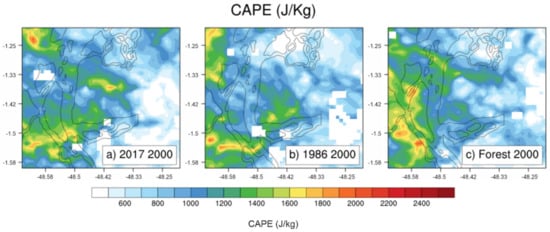
Figure 10.
Convective available potential energy (CAPE) values simulated by the model for each scenario in 2000.
The urban characteristics change the local energy budget. More sensible heat is emitted to the atmosphere by the cities, resulting in a higher air temperature near the surface and a higher CAPE [52,53]. The 2017 and 1986 runs presented a higher upward sensible heat flux than the forest scenario results (Figure 11). However, the size of the medium density area and the characteristics of the high-density slums and high-density classes in the BMR center of the 2017 scenario were responsible for a stronger and more persistent sensible heat flux across the BMR domain, compared to that of the 1986 scenario. Meanwhile, the latent heat flux (Figure 12) of the urban scenarios was smaller than that of the forest scenario, as expected by the reduced amount of vegetation [54,55]. This higher latent flux in the forest scenario may be responsible for the similarities detected in the reflectivity shown in Figure 9 between the forest and 2017 scenarios.
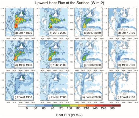
Figure 11.
Upward heat fluxes (W m−2) for each of the 2017 (a–d), 1986 (e–h), and forest (i–l) scenarios at 1930, 2000, 2030, and 2100 UTC.
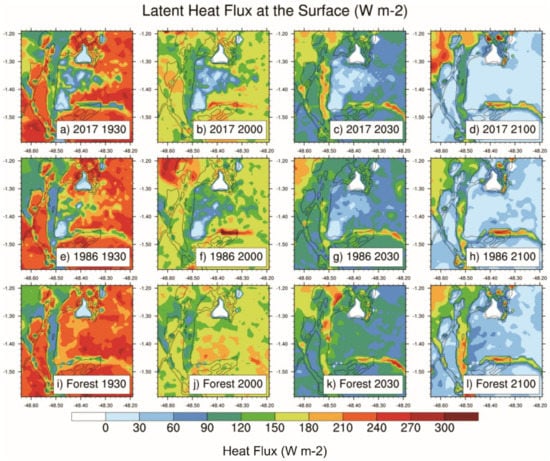
Figure 12.
Latent heat fluxes (W m−2) for each of the 2017 (a–d), 1986 (e–h), and Forest (i–l) scenarios at 1930, 2000, 2030, and 2100 UTC.
Figure 13 is a longitudinal cross-section in the middle of the BMR showing the maximum reflectivity (shade) and the vertical wind speed (contours). There was a persistent column of upward wind before the storm in the 2017 scenario. In the 1986 scenario, this was only noted at 1930 UTC and in the forest one an oscillation can be noted, alternating between the downward and upward movements. After the storm, at 2100 UTC, there was still a convective movement in both urban scenarios, but with a denser cloud in the 2017 scenario.
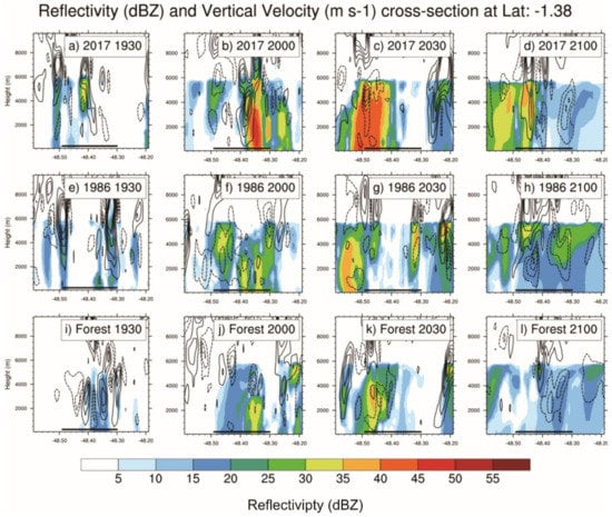
Figure 13.
Reflectivity (dBZ) values for the 2017 (a–d), 1986 (e–h), and forest (i–l) scenarios at 1930, 2000, 2030, and 2100 UTC. The dashed contours are the negative vertical wind speed, and the solid contours are positive vertical wind velocity, ranging from −5 to 5 m s−1 and an increment of 1 m s−1. The black line near the x-axis represents the BMR.
The higher wind speed in the 2017 scenario transported moisture and energy from the surface to higher altitudes, producing a deeper and larger system, as expected from Figure 9. Figure 14 indicates this transport of moisture and energy. However, the downdrafts produced by the convective circulation also brought cold and dry air from aloft, which could prevent the development of new storm cells [56]. This movement can be detected where the potential temperature reduced near the updrafts at 1930 UTC in Figure 14.
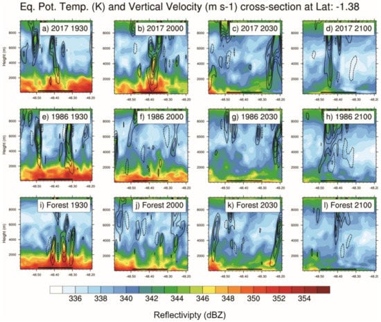
Figure 14.
Equivalent potential temperatures (K) for the 2017 (a–d), 1986 (e–h), and forest (i–l) scenarios at 1930, 2000, 2030, and 2100 UTC. The dashed contours are the negative vertical wind speed, and the solid contours are the positive vertical wind velocity, ranging from −5 to 5 m s−1 and an increment of 1 m s−1. The black line near the x-axis represents the BMR.
Despite this transport of cold and dry air to the surface (below 2000 m), as the water from precipitation fell from the clouds it could evaporate and be transported back up by the cold pool circulation, in the wake of the storm, and be used as fuel for the generation of new cell or keep the old one alive for a longer time [57,58]. The 2017 scenario displayed a situation that can be a result of this process, as the system was still present at 2100 UTC.
Aside from the energy budget, the urban characteristics can change other atmospheric variables that have an important role in storm development such as the surface roughness length.
The different building heights that compose an urban landscape increase the surface roughness length and reduce the wind speed across the BMR, keeping the system for a longer period inside the region and allowing it to grow stronger [59,60]. Figure 15 shows the vertical profile of the wind speed in the atmosphere. The forest scenario had a more homogeneous surface, which reduced the roughness, and the wind was faster. However, with urbanization and the barrier effect caused by the buildings, the wind got slower near the surface, below 3 m s−1 for the 2017 and 1986 scenarios, while the wind in the forest scenario reached above 5 m s−1 at all considered times (from the ground up to 2000 m). The urban effect also increased the vertical wind shear, which was stronger in urban scenarios.
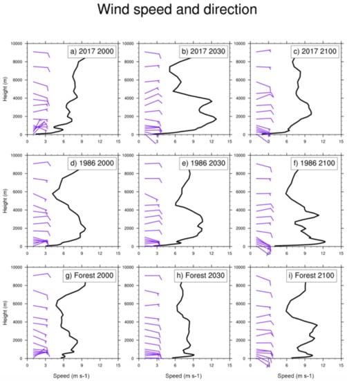
Figure 15.
Wind speed (solid line) and wind direction (barbs) vertical profiles for each scenario at 2000, 2030, and 2100 UTC.
As CAPE, the wind shear is another important element of storm development. If both forces are well balanced, with a moderate shear—associated with a cold pool propagated by the storm downdraft that brings dry and cold air from above the clouds to the surface [58,61,62]—and sufficiently high CAPE, new storms can develop right in front of the old one, keeping the system active for a longer period [48,63]. When these forces are out of balance, the storm structure can change, leading to the system split and/or underdevelopment [64,65].
The increased surface roughness also contributes to the convergence of moisture and heat at the surface, maintaining the storm active for a longer time [60,66,67,68]. Figure 16 shows that the wind speed at 10 m above ground was always higher (reaching up to 7 m s−1) in the forest scenario than in the urban ones (where the speed barely reached 4 m s−1), and the 2017 wind speed was slower than in 1986, especially before the storm, at 2000 UTC. The reduced velocity in the 2017 scenario favored convergence at the surface, as can be seen by the size and direction of the arrows and the color shading. Meanwhile, the wind in the 1986 scenario pushed more heat and moisture downstream, resulting in the positioning of the system southward of the BMR. After the storm, the wind assumed a north-easterly direction in all three scenarios, but it was still slower in 2017.
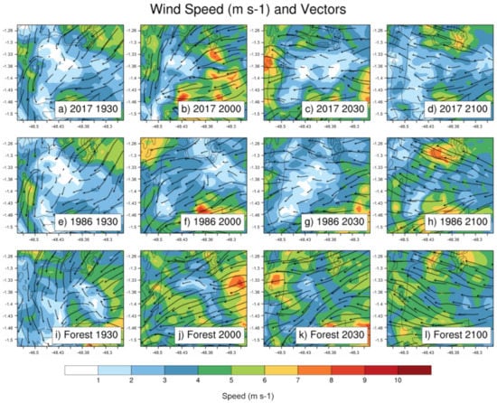
Figure 16.
Wind vector fields near the surface for each scenario at 1930, 2000, 2030, and 2100 UTC.
4. Conclusions
The WRF ensemble means simulated reasonably well the storm that occurred on 7 June 2011. Even though some differences were observed between the ensemble mean, radiosonde, and radar data, the ensemble mean estimated the correct time and position of the event, allowing an evaluation of the storm structure in different land use/cover scenarios.
The results presented here showed that, although the urban area has not expanded significantly, its composition has changed, and the urban characteristics of BMR in 2017 can influence the development of meteorological systems in this region. The higher availability of convective energy and the reduced wind speed, which favored confluence and vertical wind shear, created a favorable environment for the enhancement of mesoscale systems over the BMR. With a smaller urban area (the 1986 scenario), the system was positioned downwind, since the higher wind speed and the reduced sensible and latent heat fluxes prevent it to develop over the BMR. If the BMR was removed and replaced with forest, the latent heat flux may be responsible for the storm positioning similar to the 2017 scenario, but the low CAPE and confluence at the surface produced a weaker storm.
While previous urban climate studies for the BMR region have shown some climate changes (due to urbanization or other factors), this work is the first one to approach the urban effect from a three-dimensional point of view, adding significant new information not only for urban researchers, but also for decision-makers, since this kind of information can be used to reduce the risks associated with thunderstorms, with actions such as allocation of resources towards areas that are becoming vulnerable to floods and creation of a thunderstorm warning system to prevent human/material damages or even to increase green areas to reduce the amount of heat available to the thunderstorm.
Supplementary Materials
The following are available online at https://www.mdpi.com/article/10.3390/atmos13071026/s1, Figure S1: accumulated precipitation (mm) at 20:00 UTC for each ensemble member (first three columns) and the ensemble mean (rightmost column) for each land use/cover scenario (rows).
Author Contributions
Conceptualization, J.V.d.O. and J.C.; methodology, J.V.d.O. and J.C.; software, J.V.d.O.; validation, J.V.d.O., J.C., M.B. and M.A.S.D.; formal analysis, J.V.d.O.; investigation, J.V.d.O. and J.C.; data curation, J.V.d.O.; writing—original draft preparation, J.V.d.O.; writing—review and editing, J.V.d.O., J.C., M.B. and M.A.S.D.; visualization, J.V.d.O.; funding acquisition, J.C. All authors have read and agreed to the published version of the manuscript.
Funding
The APC was funded by the Pró-reitoria de Pesquisa e Pós-Graduação/Universidade Federal do Pará (PROPESP/UFPA) - PAPQ (Programa de Apoio à Publicação Qualificada), Edital 02/2022.
Acknowledgments
Juarez Ventura de Oliveira would like to thank the Programa de Doutorado Sanduiche (PDSE) from the Coordenação de Aperfeiçoamento de Pessoal de Nível Superior (CAPES) for the scholarship (process number: 88881.186837/2018-01). The authors would like to thank the Chuva Project for the data used in this research, NCAR for providing support and infrastructure to Juarez Ventura de Oliveira during the PDSE visit, and Pró-reitoria de Pesquisa e Pós-Graduação/Universidade Federal do Pará (PROPESP/UFPA) (PAPQ, Programa de Apoio à Publicação Qualificada) the necessary support during the manuscript preparation and submission.
Conflicts of Interest
The authors declare no conflict of interest.
References
- Howard, L. The Climate of London; International Association for Urban Climate: London, UK, 2008; p. 285. Available online: http://urban-climate.org/documents/LukeHoward_Climate-of-London-V1.pdf (accessed on 20 April 2022).
- Shepherd, J.M. A Review of Current Investigations of Urban-Induced Rainfall and Recommendations for the Future. Earth Interact. 2005, 9, 1–27. [Google Scholar] [CrossRef]
- Zhang, D.-L. Rapid urbanization and more extreme rainfall events. Sci. Bull. 2020, 65, 516–518. [Google Scholar] [CrossRef]
- Chen, F.; Yang, X.; Zhu, W. WRF simulations of urban heat island under hot-weather synoptic conditions: The case study of Hangzhou City, China. Atmos. Res. 2014, 138, 364–377. [Google Scholar] [CrossRef]
- Jenerette, G.D.; Harlan, S.L.; Brazel, A.; Jones, N.; Larsen, L.; Stefanov, W.L. Regional relationships between surface temperature, vegetation, and human settlement in a rapidly urbanizing ecosystem. Landsc. Ecol. 2007, 22, 353–365. [Google Scholar] [CrossRef]
- Pyrgou, A.; Santamouris, M.; Livada, I. Spatiotemporal Analysis of Diurnal Temperature Range: Effect of Urbanization, Cloud Cover, Solar Radiation, and Precipitation. Climate 2019, 7, 89. [Google Scholar] [CrossRef]
- Guo, G.; Wu, Z.; Xiao, R.; Chen, Y.; Liu, X.; Zhang, X. Impacts of urban biophysical composition on land surface temperature in urban heat island clusters. Landsc. Urban Plan. 2015, 135, 1–10. [Google Scholar] [CrossRef]
- Herold, N.; Kala, J.; Alexander, L.V. The influence of soil moisture deficits on Australian heatwaves. Environ. Res. Lett. 2016, 11, 064003. [Google Scholar] [CrossRef]
- Sati, A.P.; Mohan, M. Impact of urban sprawls on thunderstorm episodes: Assessment using WRF model over central-national capital region of India. Urban Clim. 2021, 37, 100869. [Google Scholar] [CrossRef]
- Wahiduzzaman, M.; Ali, M.; Luo, J.J.; Wang, Y.; Uddin, M.; Shahid, S.; Islam, A.R.M.; Mondal, S.K.; Siddiki, U.R.; Bilal, M.; et al. Effects of convective available potential energy, temperature and humidity on the variability of thunderstorm frequency over Bangladesh. Theor. Appl. Climatol. 2022, 147, 325–346. [Google Scholar] [CrossRef]
- Ihadua, I.M.T.J.; Pereira Filho, A.J. On Thunderstorm Microphysics under Urban Heat Island, Sea Breeze, and Cold Front Effects in the Metropolitan Area of São Paulo, Brazil. Atmos. Clim. Sci. 2021, 11, 614–643. [Google Scholar]
- Georgescu, M.; Broadbent, A.M.; Wang, M.; Krayenhoff, E.S.; Moustaoui, M. Precipitation response to climate change and urban development over the continental United States. Environ. Res. Lett. 2021, 16, 044001. [Google Scholar] [CrossRef]
- Zhang, N.; Wang, Y. Mechanisms for the isolated convections triggered by the sea breeze front and the urban heat Island. Meteorol. Atmos. Phys. 2021, 133, 1143–1157. [Google Scholar] [CrossRef]
- Niyogi, D.; Lei, M.; Kishtawal, C.; Schmid, P.; Shepherd, M. Urbanization Impacts on the Summer Heavy Rainfall Climatology over the Eastern United States. Earth Interact. 2017, 21, 1–17. [Google Scholar] [CrossRef]
- Yu, M.; Liu, Y. The possible impact of urbanization on a heavy rainfall event in Beijing. J. Geophys. Res. Atmos. 2015, 120, 8132–8143. [Google Scholar] [CrossRef]
- Dixon, P.G.; Mote, T.L. Patterns and Causes of Atlanta’s Urban Heat Island–Initiated Precipitation. J. Appl. Meteorol. 2003, 42, 1273–1284. [Google Scholar] [CrossRef]
- Bornstein, R.; Lin, Q. Urban heat islands and summertime convective thunderstorms in Atlanta: Three case studies. Atmos. Environ. 2000, 34, 507–516. [Google Scholar] [CrossRef]
- Zhang, D.-L.; Jin, M.S.; Shou, Y.; Dong, C. The Influences of Urban Building Complexes on the Ambient Flows over the Washington–Reston Region. J. Appl. Meteorol. Climatol. 2019, 58, 1325–1336. [Google Scholar] [CrossRef]
- Changnon, S.A.; Semonin, R.G.; Auer, A.H.J.; Braham, R.R.J.; Hales, J.M. Metromex: A Review and Summary; Changnon, S.A., Ed.; American Meteorological Society: Boston, MA, USA, 1981; Available online: http://link.springer.com/10.1007/978-1-935704-29-4 (accessed on 20 April 2022).
- Van den Heever, S.C.; Cotton, W.R. Urban aerosol impacts on downwind convective storms. J. Appl. Meteorol. Climatol. 2007, 46, 828–850. [Google Scholar] [CrossRef]
- Dos Santos, T.V. Urban Expansion and Green Urbanism in an Amazonian Metropolis: The Production of Urbanized Nature in the Metropolitan Region of Belem. Curr. Urban Stud. 2020, 8, 623–644. [Google Scholar] [CrossRef]
- Mansur, A.V.; Brondizio, E.S.; Roy, S.; de Miranda Araújo Soares, P.P.; Newton, A. Adapting to urban challenges in the Amazon: Flood risk and infrastructure deficiencies in Belém, Brazil. Reg. Environ. Chang. 2018, 18, 1411–1426. [Google Scholar] [CrossRef]
- Teixeira, E.G.S.; Costa, L.S.; Almeida, A.C. Comparação entre a variação mensal da CAPE e da precipitação em Belém, PA. In Proceedings of the Series of the Brazilian Society of Computational and Applied Mathematics, Campo Grande, Brazil, 13–17 September 2021; Available online: https://proceedings.sbmac.emnuvens.com.br/sbmac/article/viewFile/125089/3554 (accessed on 20 April 2022).
- Azevedo, S.D.; Soares, L.F.A.; Torres, L.M. Temperatura de superfície e uso e cobertura do solo em municípios da região metropolitana de Belém/PA. Rev. Ibero-Am. Ciências Ambient. 2020, 12, 214–222. [Google Scholar] [CrossRef]
- Dos Santos, T.O.; de Andrade Filho, V.S.; dos Santos França, R.; de Brito Gomes, W.; Rocha, V.M. Caracterização e variabilidade climática baseada em séries de temperatura e precipitação nos municípios de Manaus (AM) e Belém (PA). Rev. Entre-Lugar 2021, 12, 321–345. [Google Scholar] [CrossRef]
- De Oliveira, J.V.; Cohen, J.C.P.; Pimentel, M.; Tourinho, H.L.Z.; Lôbo, M.A.; Sodre, G.; Abdala, A. Urban climate and environmental perception about climate change in Belém, Pará, Brazil. Urban Clim. 2020, 31, 100579. [Google Scholar] [CrossRef]
- Silva Junior, C.H.L.; Pessôa, A.C.M.; Carvalho, N.S.; Reis, J.B.C.; Anderson, L.O.; Aragão, L.E.O.C. The Brazilian Amazon deforestation rate in 2020 is the greatest of the decade. Nat. Ecol. Evol. 2021, 5, 144–145. [Google Scholar] [CrossRef]
- Alves de Oliveira, B.F.; Bottino, M.J.; Nobre, P.; Nobre, C.A. Deforestation and climate change are projected to increase heat stress risk in the Brazilian Amazon. Commun. Earth Environ. 2021, 2, 207. [Google Scholar] [CrossRef]
- INMET. INMET Clima. 2020. Available online: http://www.inmet.gov.br/portal/index.php?r=clima/graficosClimaticos (accessed on 12 January 2020).
- Xu, H. Extraction of Urban Built-up Land Features from Landsat Imagery Using a Thematicoriented Index Combination Technique. Photogramm. Eng. Remote Sens. 2007, 73, 1381–1391. Available online: https://www.ingentaconnect.com/content/asprs/pers/2007/00000073/00000012/art00006 (accessed on 20 April 2022). [CrossRef]
- Sekertekin, A.; Abdikan, S.; Marangoz, A.M. The acquisition of impervious surface area from LANDSAT 8 satellite sensor data using urban indices: A comparative analysis. Environ. Monit. Assess. 2018, 190, 381. [Google Scholar] [CrossRef]
- Souza, D.O. Influencia da Ilha de Calor Urbana nas Cidades de Manaus e Belem Sobre o Microclima Local; National Institute for Space Research: State of São Paulo, Brazil, 2012. [Google Scholar]
- Machado, L.A.T.; Dias, M.A.F.; Morales, C.; Fisch, G.; Vila, D.; Albrecht, R.; Goodman, S.J.; Calheiros, A.J.; Biscaro, T.; Kummerow, C.; et al. The CHUVA project: How does convection vary across Brazil? Bull. Am. Meteorol. Soc. 2014, 95, 1365–1380. [Google Scholar] [CrossRef]
- Skamarock, W.C.; Klemp, J.B.; Dudhia, J.; Gill, D.O.; Barker, D.M.; Wang, W.; Powers, J.G. A Description of the Advanced Research WRF Version 3; NCAR Technical Note; University Corporation for Atmospheric Research: Boulder, CO, USA, 2008. [Google Scholar]
- GFS—Global Forecast System. Available online: https://www.emc.ncep.noaa.gov/emc/pages/numerical_forecast_systems/gfs.php (accessed on 20 April 2022).
- MUR—Multi-scale Ultra-high Resolution. Available online: https://podaac.jpl.nasa.gov/MEaSUREs-MUR (accessed on 20 April 2022).
- WRFDA. WRF Data Assimilation System Users Page. Available online: https://www2.mmm.ucar.edu/wrf/users/wrfda/index.html (accessed on 20 April 2022).
- Ferrier, B.S.; Lin, Y.; Black, T.; Rogers, E.; DiMego, G. Implementation of a new grid-scale cloud and precipitation scheme in the NCEP Eta model. In Proceedings of the 19th Conference on Weather Analysis and Forecasting/15th Conference on Numerical Weather Prediction Seattle, Philadelphia, PA, USA, 11–16 August 2002; American Meteorological Society: Boston, MA, USA, 2002. Available online: https://ams.confex.com/ams/SLS_WAF_NWP/webprogram/Paper47241.html (accessed on 20 April 2022).
- Iacono, M.J.; Delamere, J.S.; Mlawer, E.J.; Shephard, M.W.; Clough, S.A.; Collins, W.D. Radiative forcing by long-lived greenhouse gases: Calculations with the AER radiative transfer models. J. Geophys. Res. Atmos. 2008, 113, 2–9. [Google Scholar] [CrossRef]
- Mlawer, E.J.; Taubman, S.J.; Brown, P.D.; Iacono, M.J.; Clough, S.A. Radiative transfer for inhomogeneous atmospheres: RRTM, a validated correlated-k model for the longwave. J. Geophys. Res. Atmos. 1997, 102, 16663–16682. [Google Scholar] [CrossRef]
- Janjić, Z.I. The surface layer in the NCEP Eta model. In Eleventh Conference on Numerical Weather Prediction; American Meteorological Society: Norfolk, VA, USA; Vancouver, BC, Canada, 1996; pp. 354–355. [Google Scholar]
- Janjić, Z.I. The Step-Mountain Eta Coordinate Model: Further Developments of the Convection, Viscous Sublayer, and Turbulence Closure Schemes. Mon. Weather Rev. 1994, 122, 927–945. [Google Scholar] [CrossRef]
- Chen, F.; Mitchell, K.; Schaake, J.; Xue, Y.; Pan, H.L.; Koren, V.; Duan, Q.Y.; Ek, M.; Betts, A. Modeling of land surface evaporation by four schemes and comparison with FIFE observations. J. Geophys. Res. Atmos. 1996, 101, 7251–7268. [Google Scholar] [CrossRef]
- Martilli, A.; Clappier, A.; Rotach, M.W. An urban surface exchange parameterisation for mesoscale models. Bound.-Layer Meteorol. 2002, 104, 261–304. [Google Scholar] [CrossRef]
- Richardson, H.; Basu, S.; Holtslag, A.A.M. Improving Stable Boundary-Layer Height Estimation Using a Stability-Dependent Critical Bulk Richardson Number. Bound.-Layer Meteorol. 2013, 148, 93–109. [Google Scholar] [CrossRef]
- Song, F.; Zhang, G.J.; Ramanathan, V.; Leung, L.R. Trends in surface equivalent potential temperature: A more comprehensive metric for global warming and weather extremes. Proc. Natl. Acad. Sci. USA 2022, 119, e2117832119. [Google Scholar] [CrossRef]
- Yin, J.; Zhang, D.-L.; Luo, Y.; Ma, R. On the Extreme Rainfall Event of 7 May 2017 over the Coastal City of Guangzhou. Part I: Impacts of Urbanization and Orography. Mon. Weather Rev. 2020, 148, 955–979. [Google Scholar] [CrossRef]
- Weisman, M.L.; Klemp, J.B. The dependece of numerically simulated convective storms on vertical wind shear and buoyancy. Mon. Weather Rev. 1982, 110, 504–520. [Google Scholar] [CrossRef]
- Garstang, M.; White, S.; Shugart, H.H.; Halverson, J. Convective cloud downdrafts as the cause of large blowdowns in the Amazon rainforest. Meteorol. Atmos. Phys. 1998, 67, 199–212. [Google Scholar] [CrossRef]
- Rogash, J.A.; Racy, J. Some Meteorological Characteristics of Significant Tornado Events Occurring in Proximity to Flash Flooding. Weather Forecast. 2002, 17, 155–159. [Google Scholar] [CrossRef]
- Van Klooster, S.L.; Roebber, P.J. Surface-based convective potential in the contiguous United States in a business-as-usual future climate. J. Clim. 2009, 22, 3317–3330. [Google Scholar] [CrossRef]
- Holley, D.M.; Dorling, S.R.; Steele, C.J.; Earl, N. A climatology of convective available potential energy in Great Britain. Int. J. Climatol. 2014, 34, 3811–3824. [Google Scholar] [CrossRef]
- Yu, Z.; Chen, T.; Yang, G.; Sun, R.; Xie, W.; Vejre, H. Quantifying seasonal and diurnal contributions of urban landscapes to heat energy dynamics. Appl. Energy 2020, 264, 114724. [Google Scholar] [CrossRef]
- Alexandri, E.; Jones, P. Temperature decreases in an urban canyon due to green walls and green roofs in diverse climates. Build. Environ. 2008, 43, 480–493. [Google Scholar] [CrossRef]
- Perini, K.; Magliocco, A. Effects of vegetation, urban density, building height, and atmospheric conditions on local temperatures and thermal comfort. Urban For. Urban Green. 2014, 13, 495–506. [Google Scholar] [CrossRef]
- Richards, D.; Fung, T.; Belcher, R.; Edwards, P. Differential air temperature cooling performance of urban vegetation types in the tropics. Urban For. Urban Green. 2020, 50, 126651. [Google Scholar] [CrossRef]
- Klemp, J.B.; Wilhelmson, R.B.; Ray, P.S. Observed and Numerically Simulated Structure of a Mature Supercell Thunderstorm. J. Atmos. Sci. 1981, 38, 1558–1580. [Google Scholar] [CrossRef][Green Version]
- Drager, A.J.; van den Heever, S.C. Characterizing convective cold pools. J. Adv. Model. Earth Syst. 2017, 9, 1091–1115. [Google Scholar] [CrossRef]
- Li, Z.; Zuidema, P.; Zhu, P. Simulated Convective Invigoration Processes at Trade Wind Cumulus Cold Pool Boundaries. J. Atmos. Sci. 2014, 71, 2823–2841. [Google Scholar] [CrossRef]
- Lin, C.Y.; Chen, W.C.; Liu, S.C.; Liou, Y.A.; Liu, G.R.; Lin, T.H. Numerical study of the impact of urbanization on the precipitation over Taiwan. Atmos. Environ. 2008, 42, 2934–2947. [Google Scholar] [CrossRef]
- Melo, A.M.Q.; Dias-Junior, C.Q.; Cohen, J.C.P.; Sá, L.D.A.; Cattanio, J.H.; Kuhn, P.A.F. Ozone transport and thermodynamics during the passage of squall line in Central Amazon. Atmos. Environ. 2019, 206, 132–143. [Google Scholar] [CrossRef]
- Tompkins, A.M. Organization of Tropical Convection in Low Vertical Wind Shears: The Role of Cold Pools. J. Atmos. Sci. 2001, 58, 1650–1672. [Google Scholar] [CrossRef]
- Rotunno, R.; Klemp, J.B.; Weisman, M.L. A Theory for Strong, Long-Lived Squall Lines. J. Atmos. Sci. 1988, 45, 463–485. [Google Scholar] [CrossRef]
- Miao, S.; Chen, F.; Li, Q.; Fan, S. Impacts of urban processes and urbanization on summer precipitation: A case study of heavy rainfall in Beijing on 1 August 2006. J. Appl. Meteorol. Climatol. 2011, 50, 806–825. [Google Scholar] [CrossRef]
- Niyogi, D.; Pyle, P.; Lei, M.; Arya, S.P.; Kishtawal, C.M.; Shepherd, M.; Chen, F.; Wolfe, B. Urban modification of thunderstorms: An observational storm climatology and model case study for the Indianapolis urban region. J. Appl. Meteorol. Climatol. 2011, 50, 1129–1144. [Google Scholar] [CrossRef]
- Shepherd, J.M. Impacts of urbanization on precipitation and storms: Physical insights and vulnerabilities. In Climate Vulnerability; Elsevier: Amsterdam, The Netherlands, 2013; pp. 109–125. Available online: https://www.srs.fs.usda.gov/pubs/48117 (accessed on 20 April 2022).
- Haberlie, A.M.; Ashley, W.S.; Pingel, T.J. The effect of urbanisation on the climatology of thunderstorm initiation. Q. J. R. Meteorol. Soc. 2015, 141, 663–675. [Google Scholar] [CrossRef]
- Varquez, A.C.G.; Nakayoshi, M.; Kanda, M. The Effects of Highly Detailed Urban Roughness Parameters on a Sea-Breeze Numerical Simulation. Bound. -Layer Meteorol. 2014, 154, 449–469. [Google Scholar] [CrossRef]


Publisher’s Note: MDPI stays neutral with regard to jurisdictional claims in published maps and institutional affiliations. |
© 2022 by the authors. Licensee MDPI, Basel, Switzerland. This article is an open access article distributed under the terms and conditions of the Creative Commons Attribution (CC BY) license (https://creativecommons.org/licenses/by/4.0/).