The Influence of Extratropical Weather Regimes on Wintertime Temperature Variations in the Arctic during 1979–2019

Abstract

In this study, the Arctic sea ice cover in the sector 30° W–60° E in February, and the monthly mean temperature (averaged over the polar cap north of 70° N and 700–1000 hPa, Tcap) in winter during 1979–2019 were analyzed using established change-point detection methods. Step changes were found in 2004, with lower sea ice cover and higher air temperature during 2005–2019 than 1979–2004 (with Tcap anomalies of 1.05 K and −0.63 K, respectively). Two combinations of weather regimes were associated with the anomalously warm months (1.61 K): (1) Scandinavian trough and Ural blocking, and (2) Atlantic ridge and Ural blocking. The first causes a “polar express” for the poleward transport of heat and moisture from mid-latitude East Europe. The second causes a “two-stage heat pump” that transports heat and moisture from the subarctic Atlantic. Their opposite combinations were associated with the anomalously cold months (−0.73 K), which occurred more frequently during 1979–2004. These trends in weather regimes could account for 25% of the step-change in Arctic winter temperature, with the remainder likely caused by changes in sea ice cover, ocean heat transport, and concentrations of aerosol and greenhouse gases.

1. Introduction

Large-scale weather regimes are recurring patterns of atmospheric circulation that typically persist for several days to two weeks and are known to organize midlatitude storms [1,2,3,4]. These patterns each appear at nearly fixed geographical locations and are often characterized in terms of persistent anomalies in mid-tropospheric geopotential height fields [5,6,7,8].

Numerous studies have described extratropical weather regimes in the Northern Hemisphere (NH) and their impact on weather and climate in the Arctic, Eurasia, and North America [9,10,11,12]. For instance, a warm Arctic and cold Eurasia (WACE) pattern is found to be associated with positive sea level pressure anomalies over western Siberia, which have become more frequent in recent years perhaps due to the observed decrease in Arctic sea ice [13,14].

Recent studies have shown that the reduction of sea ice in the Barents Sea and the Kara Sea enhances air temperature over the areas due to heat and moisture released from the open water, with the increased water vapor and clouds trapping infrared radiation which warms the Arctic [15,16,17,18]. Modeling studies show that the positive atmospheric feedbacks may suppress the growth of sea ice in winter, followed by earlier melting in spring and reduced sea ice albedo in summer, and may cause further reduction of sea ice in winter in future warming scenarios [19,20,21]. It is tempting to find a tipping point for the Arctic environment that may emerge from this feedback loop and the temperature threshold for seawater freezing.

The purpose of this study is to take another look at the relationships between the extratropical weather regimes and air temperature in the Arctic and between sea ice cover (SIC) and air temperature. The paper is organized as follows. The data sets and analyses are described in Section 2. Section 3 presents a breakpoint analysis of sea ice cover and air temperature in the Arctic in winter during 1979–2019. The NH extratropical weather regimes are characterized in Section 4. The Arctic impact of the weather regimes are presented in Section 5. A summary of results is given in Section 6.

2. Data and Analyses

Daily mean 500 hPa geopotential height (z500) fields are used in this study for the characterization of weather regimes. The data are derived from the National Center for Environmental Prediction and National Center for Atmospheric Research (NCEP-NCAR) reanalysis (NCEP1) [22], NCEP and Department of Energy (NCEP-DOE) reanalysis (NCEP2) [23], and from the European Center for Medium-Range Weather Forecasts (ECMWF) interim reanalysis (ERA-Interim) [24]. The NCEP1 and NCEP2 data were retrieved from the website (https://www.esrl.noaa.gov/psd/data/gridded/reanalysis/; accessed on 28 September 2020) and have a horizontal resolution of 2.5° × 2.5° latitude by longitude. The ERA-Interim data were retrieved from the ECMWF data server (https://apps.ecmwf.int/datasets/; accessed on 16 July 2019) at a resolution of 0.75° × 0.75° and regridded to 2.25° × 2.25° latitude by longitude. A total of forty cold seasons (November to March, or NDJFM) are available from November 1979 to March 2019.

Monthly mean air temperatures from NCEP reanalysis were averaged over the polar cap (north of 70° N) for the lower troposphere (700 hPa—the surface, Tcap) and middle troposphere (400–700 hPa), weighted by area and pressure thickness, (i.e., mass) of each grid box, with the air temperature at the center of each grid estimated by linear interpolation. Seasonal averages of Tcap were calculated for December–February (DJF). Monthly sea ice concentration data (in 25 km × 25 km grid) was obtained from the NOAA National Snow and Ice Data Center (NSIDC, https://nsidc.org/data/g02202/; accessed on 23 September 2020) [25,26]. Two different R packages were downloaded (URL https://github.com/rkillick/changepoint/; accessed on 10 January 2022 and https://cran.r-project.org/web/packages/strucchange/; accessed on 10 January 2022) downloaded that have implemented various methods for the optimal identification of break-points in a time series [27,28,29].

In this study, the “changepoint” package of R (ver. 2.2.2) was used to estimate the shifting of mean state and point of shift in sea ice and air temperature, using the “MBIC” (modified Bayes information criterion) and the “AMOC” (at most one changepoint) options. Similarly, the “strucchange” package of R (ver. 1.5–2) was used to estimate the breakpoints in regression relationships, (e.g., the optimal partition of linear trends). The same break-point was identified by these methods for each time series: 2004 for winter mean Tcap and for February SIC in the 30° W–60° E sector (the Greenland Sea, the Norwegian Sea, and the Barents Sea, extending to the North Pole). Changes in winter SIC are also large in the Kara Sea but are small in other sectors. February SIC best reflects the production of ice integrated over the winter season. A large climate change in the Arctic at the time about 2004 has been reported in previous studies [30,31].

Daily height data were averaged by day of the year to yield the mean annual cycles for the period of 1979–2019. Daily height anomalies were calculated by subtracting the mean annual cycles, which retain interannual, intra-seasonal, and synoptic variations. An EOF analysis was performed for NDJFM (151 days × 40 years) for the height anomalies in the Atlantic–Eurasia sector (AEA: 60° W–150° E and north of 30° N), and another for the Pacific-North America sector (PNA: 150° E–60° W and north of 30° N). This does not consider any lateral shifts of the EOF patterns over time [32]. Separate EOF analyses for the two sectors are designed to maximize local variances explained by the EOFs and to eliminate the requirement of synchronization of patterns between the sectors when they are combined [33]. Results for the PNA sector will be reported in a separate paper.

An EOF analysis finds a set of independent spatial patterns (the EOFs) such that the time evolution of a spatial variable, (e.g., 2-dimensional height anomalies) can be reconstructed as the sum of the product of the EOFs and corresponding expansion coefficients at each time step. The time series of expansion coefficients are referred to as principal components (PCs). The PC values are normalized by the respective standard deviations (s. d.) over the total number of days. No rotation of the principal components is performed as customary in hemisphere EOF analyses [7].

The EOFs are uncorrelated in space and the PCs are uncorrelated in time. However, when the daily expansion coefficients are averaged over a month or a season, the mean PCs may become partially correlated because the daily PCs may be correlated when two time series are shifted in time relative to each other (results not shown). A lagged correlation occurs when one pattern is preferentially transitioned to another pattern, such as resulting from Rossby wave propagation, or two patterns tend to respond to a common disturbance but at different times within a month/season. The daily PC values may be positively or negatively cross correlated for sub-periods.

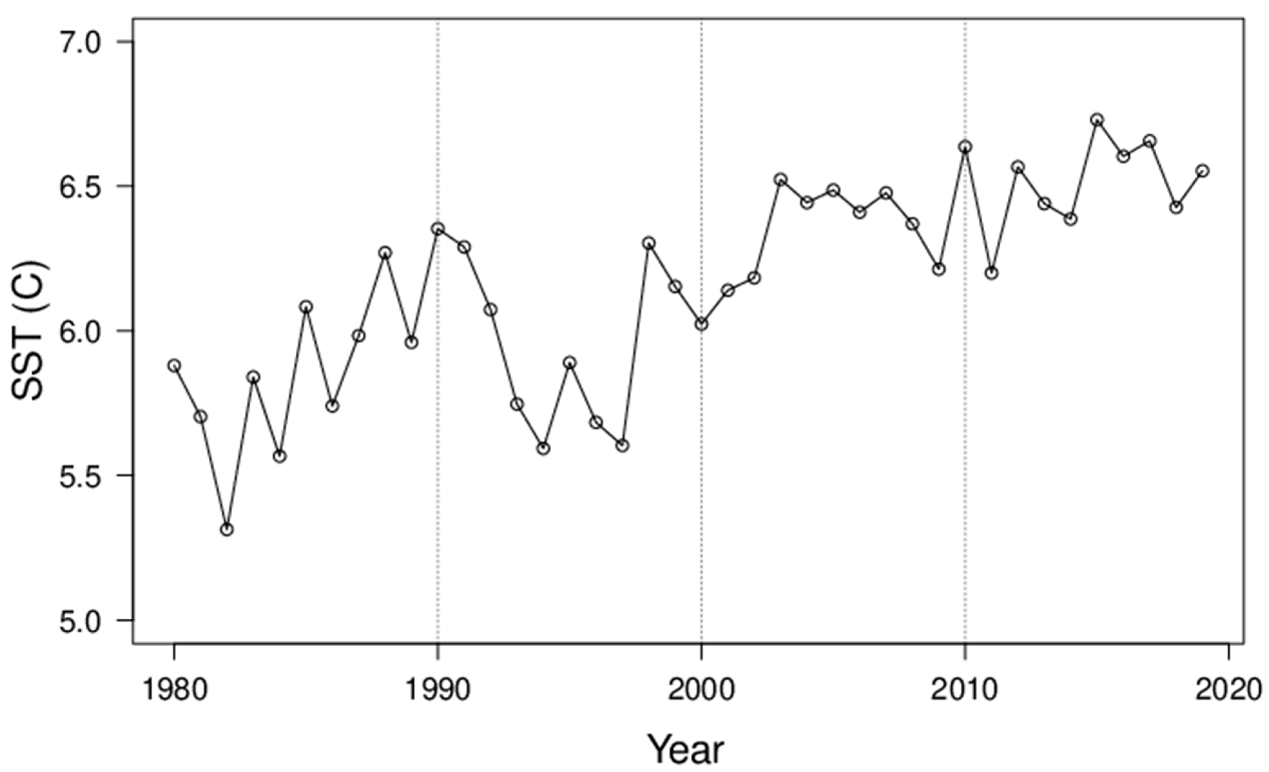
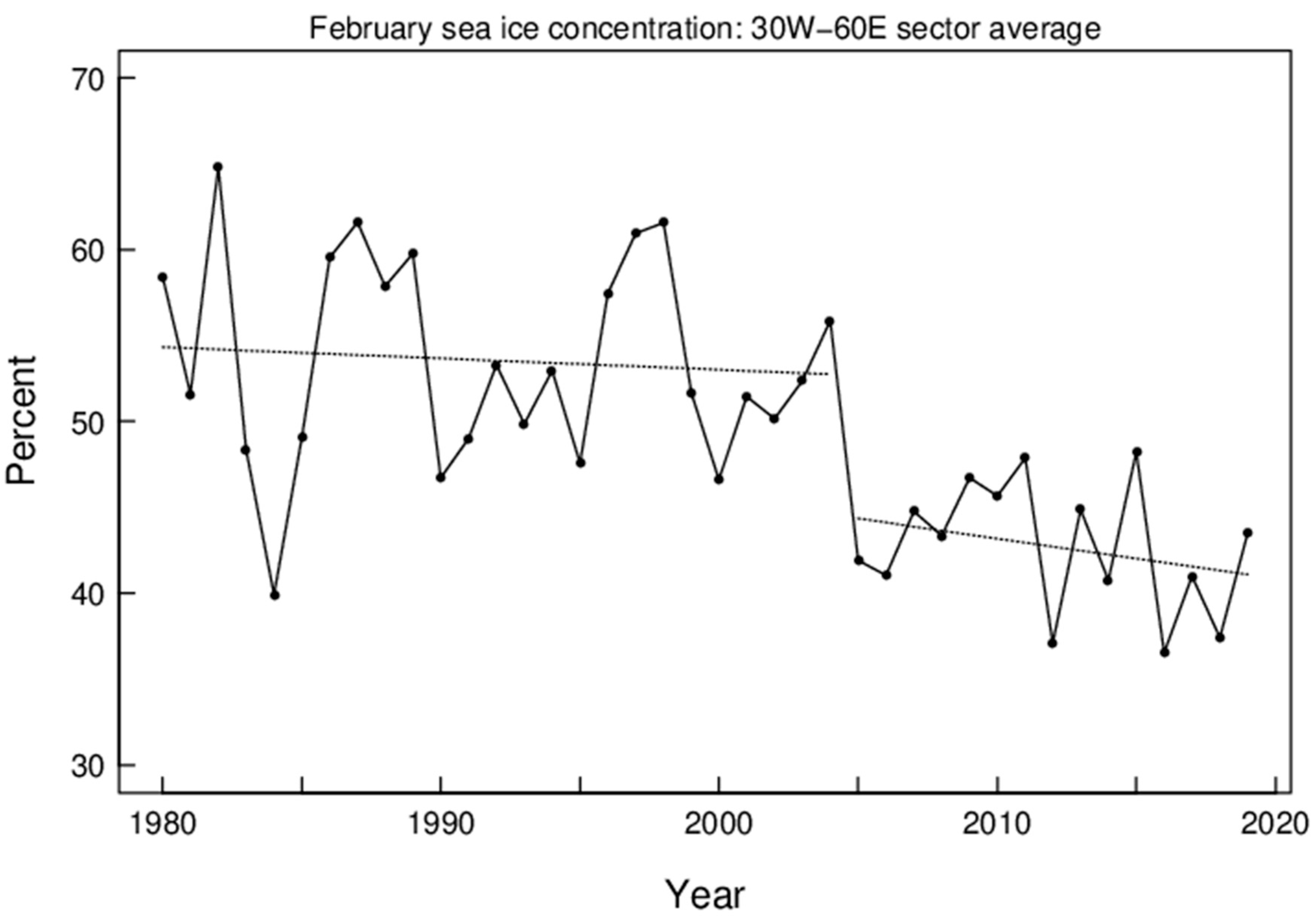
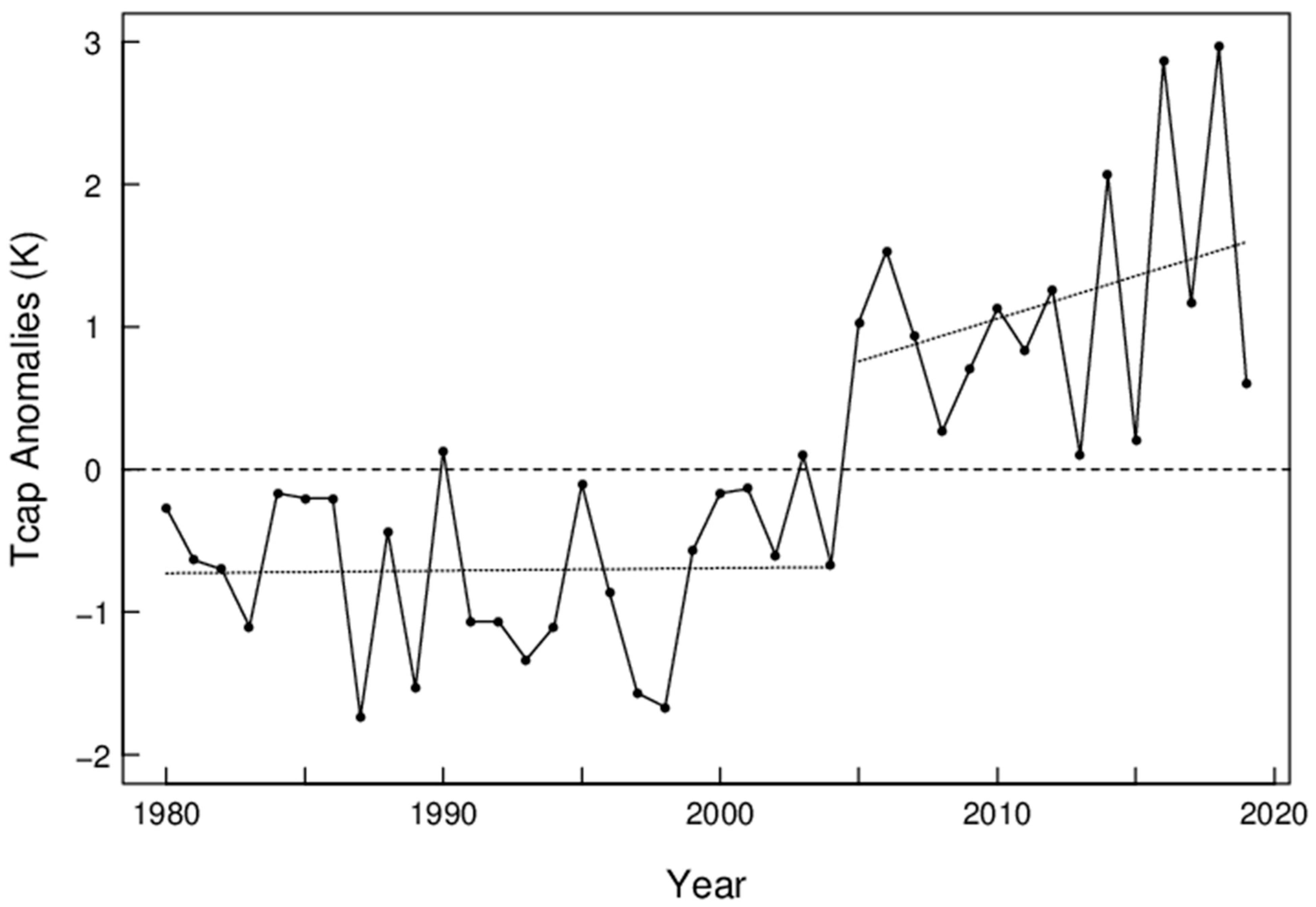
3. Step-Changes in Sea Ice and Arctic Temperature

The largest decreases in sea ice concentration in winter have occurred in the region covering the Greenland Sea, the Norwegian Sea, and the Barents Sea (the Nordic seas), which is also in the main path of moisture intrusions into the Arctic during winter [34]. Figure 1 shows the February sea ice concentration in the sector from 30° W to 60° E. Straight lines show the linear regressions for the two periods before and after the break-point, respectively, with a step-change of sea ice concentration, from 53% to 44%, at the break-point. The root-mean-squared (RMS) errors are 6.0% and 3.6% for the first and second time periods, respectively. The negative trend (%/year) is greater in magnitude in the second than the first period (−0.23 ± 0.22 s.e. and −0.066 ± 0.17, respectively), although statistically insignificant (Figure 1). The DJF mean Tcap anomalies are shown in Figure 2, in which a step-change of Tcap (1.45 K) is objectively determined as for sea ice. A trend of near-zero is shown for Tcap from 1980–2004 (January year), and a positive trend (0.06 K/year) from 2005–2019. The step-changes shown in Figure 1 and Figure 2 may indicate a cause-and-effect relationship between the SIC in the Nordic seas and Tcap and/or responses to a common cause. For instance, a Ural blocking regime has been found to be associated with winter warming and sea ice reduction in the Arctic [35,36,37]. It is interesting to examine the role of weather regimes on the observed Arctic environmental changes.

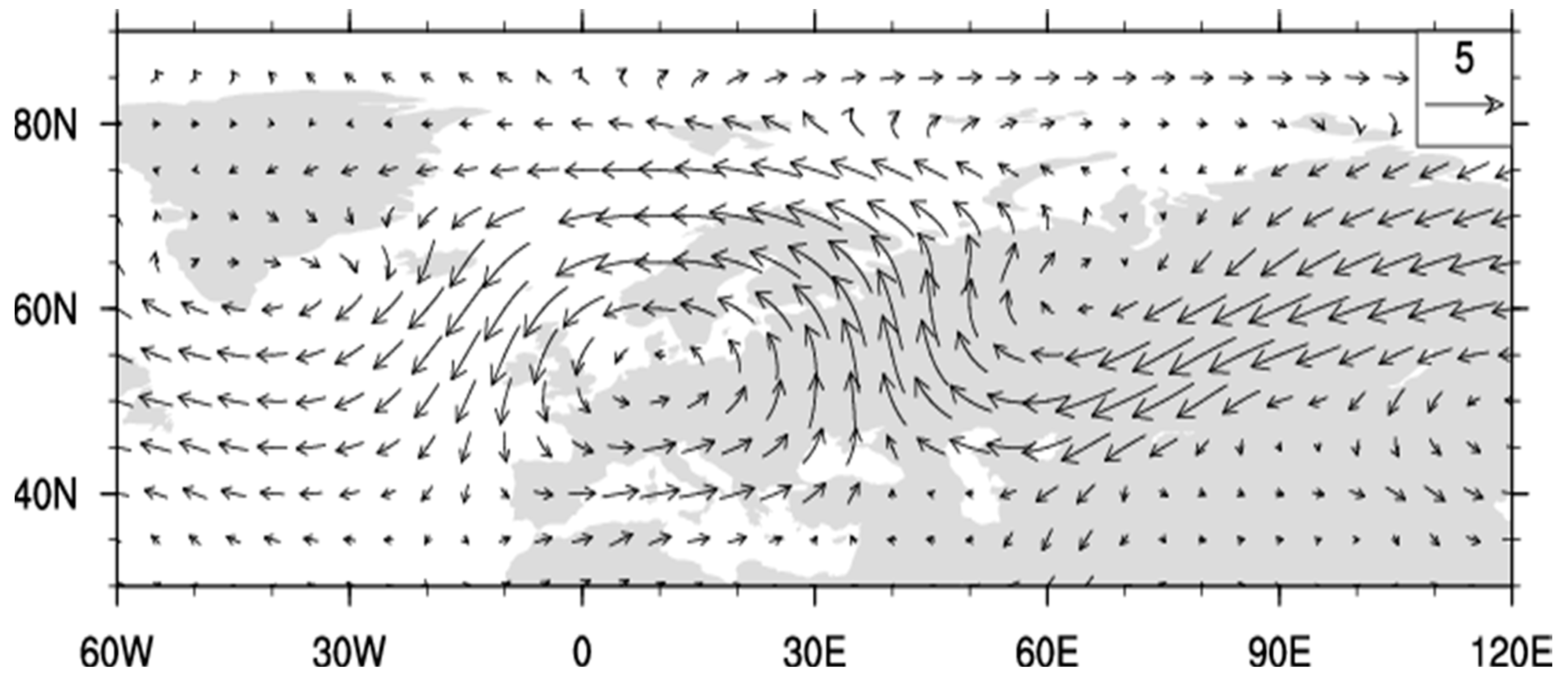
4. Characterization of Weather Regimes

Figure 3 shows the four leading EOFs in the AEA sector based on daily NCEP2 data of 500 hPa heights. The EOFs 1–4 explain 12.4%, 11.3%, 10.5%, and 8.6% of the total variance, respectively, at a total of 42.8%. These EOFs are stationary patterns with large spatial scales and their PCs exhibit long auto-correlations (1–2 weeks, results not shown) and should be well constrained by observations in all the reanalysis products. The results for NCEP1 and ERA-Interim are very similar and will not be shown in this paper to avoid redundancy and repetition. Minor EOFs, which account for the remaining, synoptic variances, will not be shown or discussed in this paper. It is noted that the leading EOFs based on monthly z500 fields account for a larger fraction of variances due to a lack of synoptic variability in the data.

The patterns are named based on their positive phases and referred to as “Greenland blocking” (GB), “Ural blocking” (UB), “Scandinavian blocking” (SB), and “Atlantic ridge” (AR). Here “blocking” is not based on the traditional definition but on the spatial and temporal scales of height anomalies. The GB resembles the negative phase of the North Atlantic oscillation (NAO), and the AR resembles the negative phase of the eastern Atlantic pattern [5]. The center (peak anomaly) of AR is about 10° (latitude) southeast of the center of GB. The SB and UB resemble Eurasia 1 and 2 patterns [5], respectively. They both show a “wave train” (low–high–low) pattern and their centers are about 35° (longitude) apart. Note that the SB and AR patterns shown in Figure 1 are similar but not the same as those defined in [38] due to different analysis domains and classification methods between the two studies.

5. Wintertime Temperature Variations in the Arctic

Polar cap temperatures (Tcap) are found to be significantly correlated with AEA sector PC2 (correlation coefficient = 0.56 and 0.50 for undetrended, DJF seasonal, and monthly averages, respectively). The correlations are insignificant for other PCs in the AEA and PNA sectors. Figure 4 shows monthly Tcap anomalies from November to March, 1979 to 2019, with red symbols indicating monthly mean PC2 > 0.2 (UB+) and PC3 < −0.2 (SB−), blue for PC2 < −0.2 (UB−) and PC3 > 0.2 (SB+), and black circles for the rest of data points, respectively. The value of 0.2 is approximately 1 standard error (s.e.) for monthly averages. The combination of SB− and UB+ regimes were found to explain the largest Tcap anomalies (red dots in Figure 4). It is noted that SB− tends to have greater amplitude than UB+ during the “heat waves”. The mean Tcap anomalies are 1.61 and −0.73 K for red (UB+ and SB−) and blue (UB− and SB+) data points, respectively. The SB− regime is found to lead the UB+ regime by about 5 days in their lagged cross-correlations (results not shown). Co-occurrence of the UB+ and SB− regimes form a south–north channel west of the Ural Mountains for the poleward transport of air masses from mid-latitude East Europe (Figure A1). This causes a “polar express” for efficiently transporting warm air from East Europe. Air pollutants were found to be injected through the “channel” from East Europe into the Arctic [39,40].

Figure 5 shows monthly Tcap anomalies from November to March, 1979 to 2019, with red symbols indicating monthly mean PC2 > 0.2 (UB+) with PC3 < −0.2 (SB−) or PC4 > 0.2 (AR+), blue for PC2 < −0.2 (UB−) with PC3 > 0.2 (SB+) or PC4 < -0.2 (AR−), and black for the rest of data points, respectively. Co-occurrence of the UB+ and AR+ regimes sets up a “two-stage heat pump” for transporting warm and moist air from the sub-polar North Atlantic region into the Arctic region (Figure A2). That is, the AR prevents the normal eastward propagation of cyclones, which then take a path northeastward to the Nordic seas [41]. The warm and moist air moved northward by the cyclonic circulations during an AR+ regime is carried further into the Arctic and eastward by the anticyclonic circulation associated with a UB+ regime (Figure A2). Figure 5 also shows large interannual and intraseasonal variations which are not associated with the combined weather regimes indicated by the red and blue symbols, reflecting the large internal variability in the atmosphere and the influences of other regimes.

It is interesting to note that the dominant mode of z500 over the AEA region (GB) is not correlated to Tcap (results not shown). During a GB+ regime, northward transport (associated cyclones) occurs through the Labrador/Davis Strait/Baffin Bay pathway, with relatively cold and dry air masses. During a GB− regime, Atlantic storms originating from coastal North America migrate eastward towards mid-latitude Europe, resulting in little poleward transport of sensible and latent energy. This is similar to a previous study [42] that shows a dipole pattern of sea-level pressure in the high latitudes is highly correlated to the export of Arctic sea ice while the Arctic oscillation is not. However, an isolated Arctic becomes colder due to radiative cooling.

The mean Tcap is −0.63 K (s.d. = 1.02) during 1979–2004 and 1.05 K during 2005–2019, respectively. When the red and blue data points are excluded, the mean Tcap in Figure 4 (Figure 5) is −0.55 K (−0.50 K) and 0.73 K (0.76 K) before and after the break-point, respectively. The occurrence frequencies for blue and red symbols are 19% and 6%, respectively, in the first period, versus 13% and 24% in the second period in Figure 4. The occurrence frequencies for blue and red symbols are 28% and 13%, respectively, in the first period, versus 16% and 31% in the second period in Figure 5. The step-change excluding the red and blue points (dashed lines) is 1.26 K, compared to 1.68 K for all data points (solid lines). The change unrelated to the red and blue weather regimes is 75% (=1.26/1.68) of the total (Figure 5). Changes in weather regimes may have contributed 25% of the step-change of Tcap. This is in agreement with a previous study [18] that shows the horizontal advection of heat is critical in explaining the variability, but not the mean, of the lower tropospheric temperature. Over the Barents–Kara Seas, an analysis of the heat budget indicates that temperature increase in the lower troposphere is almost equally partitioned into turbulent flux, horizontal advection, and greenhouse effect [18].

The step-change of Tcap is found to be associated with an increase in the meridional wind (V, 100–1000 hPa) on the order of 1 m/s at 70° N in the sector from 0–60° E and a decrease in V of similar magnitude from 90° E−150° E (with smaller decreases from 60° E–90° E and 150° E–180° E; not shown). It was shown in a previous study that about 2/3 of the variance of DJF mean Tcap between 1979 and 2012 was associated with changes in the meridional winds over the Nordic region and Siberia [43]. The intrusion of warm and moist air masses from the subarctic Atlantic was found to increase downward infrared radiation and surface temperature, slowing the growth of sea ice in the Arctic [44].

The remainder (75%) of the step-change of Tcap is likely caused by the polar amplification of global warming [45], a decrease in aerosol pollution [46], and sea ice reduction [18]. The sea surface temperature [47] of the North Atlantic, averaged for DJF, 10° W–10° E and 60° N–70° N, has increased by about 0.5 K from the 1980s to the 2010s (Figure A3), which likely contributed to the long-term trends and the step-change of sea ice (Figure 1). It is likely that the reduction of sea ice and atmospheric feedback have contributed the most to the step-change in Tcap [15,16,17,18].

6. Summary

In this study, the extratropical (north of 30° N) weather regimes in the Atlantic–Eurasia sector (AEA, 60° W–150° E) were characterized by EOF analysis of daily 500 hPa geopotential heights in November–March 1979–2019. The first four leading EOFs resemble well-known teleconnection patterns. Statistical methods for the optimal identification of breakpoints were applied to the time series of Arctic winter mean temperature (north of 70° N and 700–1000 hPa, Tcap) and February sea ice cover (30° W–60° E). A step-increase in Tcap is found to correspond well with a step-decrease in the sea ice cover, both of which occurred between 2004 and 2005.

The monthly Tcap was found to be significantly correlated with the PC corresponding with the UB pattern. It is shown that the occurrences of the UB+ with AR+ or SB− patterns were associated with anomalously warm months, which were more frequent during 2005–2019. The occurrences of the UB− with AR− or SB+ regimes were associated with anomalously cold months, which were more frequent during 1979–2004. The combination of UB+ and AR+ causes a “two-stage heat pump” for transporting warm and moist air from the North Atlantic to the Arctic, while that of UB+ and SB− causes a “polar express” for the transport of warm air from East Europe. These combinations of weather regimes were associated with 25% of the step-increase in Tcap.

This study is intended to find a possible tipping point, which may emerge from a feedback loop and the temperature threshold for seawater freezing, as the sea ice continues to melt in the Arctic, and has shown examples of how Arctic climate change may occur through the weather–scale processes. It remains to be observed/determined whether the observed step-changes in sea ice and Tcap indicate a tipping point for the Arctic environment. As global warming continues, the feedback loop will expand in area, and the reduction of sea ice and the increase in air temperature is expected to be irreversible under external forcing, perhaps with the exception of a catastrophic event.

References

1. Rheinhold, B.B.; Pierrehumbert, R.T. Dynamics of weather regimes: Quasi-stationary waves and blocking. Mon. Wea. Rev. 1982, 110, 1105–1145. [Google Scholar] [CrossRef] [Green Version]
2. Robertson, A.W.; Metz, W. Transient-eddy, feedbacks derived from linear theory and observations. J. Atmos. Sci. 1990, 47, 2743–2764. [Google Scholar] [CrossRef] [Green Version]
3. Robertson, A.W.; Ghil, M. Large-scale weather regimes and local climate over the Western United States. J. Clim. 1999, 12, 1796–1813. [Google Scholar] [CrossRef]
4. Hannachi, A.; Straus, D.M.; Franzke, C.L.E.; Corti, S.; Woolings, T. Low-frequency nonlinearity and regime behavior in the Northern Hemispshere extratropical atmosphere. Rev. Geophys. 2017, 55, 199–234. [Google Scholar] [CrossRef]
5. Wallace, J.M.; Gutzler, D.S. Teleconnections in the potential height field during the Northern Hemisphere winter. Mon. Wea. Rev. 1981, 109, 784–812. [Google Scholar] [CrossRef]
6. Blackmon, M.L.; Lee, Y.-H.; Wallace, J.M.; Hsu, H.-H. Time variation of 500 mb height fluctuations with long, intermediate and short time scales as deduced from lag-correlation statistics. J. Atmos. Sci. 1984, 41, 981–991. [Google Scholar] [CrossRef] [Green Version]
7. Barnston, A.G.; Livezey, R.E. Classification, seasonality and persistence of low-frequency atmospheric circulation patterns. Mon. Wea. Rev. 1987, 115, 1083–1126. [Google Scholar] [CrossRef]
8. Rennert, K.J.; Wallace, J.M. Cross-frequency coupling, skewness, and blocking in the Northern Hemisphere winter circulation. J. Clim. 2009, 22, 5650–5666. [Google Scholar] [CrossRef] [Green Version]
9. Roundy, P.E.; MacRitchie, K.; Asuma, J.; Melino, T. Modulation of the global atmospheric circulation by combined activity in the Madden-Julian Oscillation and the El Niño-Southern Oscillation during boreal winter. J. Clim. 2010, 23, 4045–4059. [Google Scholar] [CrossRef] [Green Version]
10. Zhang, C. Madden-Julian Oscillation: Bridging weather and climate. Bull. Am. Met. Soc. 2013, 94, 1849–1870. [Google Scholar] [CrossRef]
11. Stan, C.; Straus, D.M.; Frederiksen, J.S.; Lin, H.; Maloney, E.D.; Schumacher, C. Review of tropical-extratropical teleconnections on intraseasonal time scales. Rev. Geophys. 2017, 55, 902–937. [Google Scholar] [CrossRef]
12. Yuan, X.; Kaplan, M.; Cane, M.A. The interconnected global climate system: A review of tropical-polar teleconnections. J. Clim. 2018, 31, 5765–5792. [Google Scholar] [CrossRef]
13. Overland, J.E.; Wang, M. Large-scale atmospheric circulation changes are associated with the recent loss of Arctic sea ice. Tellus 2010, 62, 1–9. [Google Scholar] [CrossRef] [Green Version]
14. Mori, M.; Watanabe, M.; Shiogama, H.; Inoue, J.; Kimoto, M. Robust Arctic sea-ice influence on the frequent Eurasian cold winters in past decades. Nat. Geosci. 2014, 7, 869–873. [Google Scholar] [CrossRef]
15. Screen, J.A.; Simmonds, I. Increasing fall-winter energy loss from the Arctic Ocean and its role in Arctic temperature amplification. Geophys. Res. Lett. 2010, 37, L16707. [Google Scholar] [CrossRef] [Green Version]
16. Screen, J.A.; Simmonds, I.; Deser, C.; Tomas, R. The atmospheric response to three decades of observed Arctic sea ice loss. J. Clim. 2013, 26, 1230–1248. [Google Scholar] [CrossRef] [Green Version]
17. Burt, M.A.; Randall, D.A.; Branson, M.D. Dark warming. J. Clim. 2005, 29, 705–719. [Google Scholar] [CrossRef]
18. Kim, J.-Y.; Kim, K.-Y. Relative role of horizontal and vertical processes in the physical mechanism of wintertime Arctic amplification. Clim. Dyn. 2019, 52, 6097–6107. [Google Scholar] [CrossRef] [Green Version]
19. Cao, Y.; Liang, S.; Chen, X.; He, T.; Wang, D.; Cheng, X. Enhanced wintertime greenhouse effect reinforcing Arctic amplification and initial sea-ice melting. Sci. Rep. 2017, 7, 8462. [Google Scholar] [CrossRef] [Green Version]
20. Hankel, C.; Tziperman, E. The role of atmospheric feedbacks in abrupt winter Arctic sea ice loss in future warming scenarios. J. Clim. 2021, 34, 4435–4447. [Google Scholar] [CrossRef]
21. Jenkins, M.; Dai, A. The impact of sea-ice loss on Arctic climate feedbacks and their role for Arctic amplification. Geophys. Res. Lett. 2021, 48, e2021GL094599. [Google Scholar] [CrossRef]
22. Kalnay, E.; Kanamitsu, M.; Kistler, R.; Collins, W.; Deaven, D.; Gandin, L.; Iredell, M.; Saha, S.; White, G.; Woollen, J.; et al. The NCEP/NCAR 40-Year Reanalysis Project. Bull. Amer. Meteor. Soc. 1996, 77, 437–471. [Google Scholar] [CrossRef] [Green Version]
23. Kanamitsu, M.; Ebisuzaki, W.; Woollen, J.; Yang, S.-K.; Hnilo, J.J.; Fiorino, M.; Potter, G.L. NCEP-DOE AMIP-II Reanalysis (R-2). Bull. Amer. Meteor. Soc. 2002, 83, 1631–1643. [Google Scholar] [CrossRef]
24. Dee, D.P.; Uppala, S.M.; Simmons, A.J.; Berrisford, P.; Poli, P.; Kobayashi, S.; Andrae, U.; Balmaseda, M.A.; Balsamo, G.; Bauer, D.P.; et al. The ERA-Interim reanalysis: Configuration and performance of the data assimilation system. Quart. J. Roy. Meteor. Soc. 2011, 137, 553–597. [Google Scholar] [CrossRef]
25. Meier, W.; Fetterer, F.; Savoie, M.; Mallory, S.; Duerr, R.; Stroeve, J. NAOA/NSIDC Climate Data Record of Passive Microwave Sea Ice Concentration, Version 2; National Snow and Ice Data Center: Boulder, CO, USA, 2013. [Google Scholar] [CrossRef]
26. Peng, G.; Meier, W.; Scott, D.; Savoie, M. A long-term and reproducible passive microwave sea ice concentration data record for climate studies and modeling. Earth Syst. Sci. Data 2013, 5, 311–318. [Google Scholar] [CrossRef] [Green Version]
27. Bai, J. Least squares estimation of a shift in linear processes. J. Time Ser. Anal. 1994, 15, 453–472. [Google Scholar] [CrossRef] [Green Version]
28. Chen, J.; Gupta, A.K. Parametric Statistical Change Point Analysis: With Applications to Genetics, Medicine, and Finance; Springer: Berlin/Heidelberg, Germany, 2012; pp. 212–215. [Google Scholar]
29. Zeileis, A.; Kleiber, C.; Krämer, W.; Hornik, K. Testing and dating of structural changes in practice. Comput. Stat. Data Anal. 2003, 44, 109–123. [Google Scholar] [CrossRef] [Green Version]
30. Zhang, X.; Lu, C.; Guan, Z. Weakened cyclones, intensified anticyclones and recent extreme cold winter weather events in Eurasia. Environ. Res. Lett. 2012, 7, 044044. [Google Scholar] [CrossRef]
31. Feng, C.; Wu, B. Enhancement of Arctic winter warming by the Siberian high over the past decade. Atmos. Ocean. Sci. Lett. 2015, 8, 257–263. [Google Scholar] [CrossRef]
32. Sung, M.-K.; Jang, H.-Y.; Kim, B.-M.; Yeh, S.-W.; Choi, Y.-S.; Yoo, C. Tropical influence on the North Pacific Oscillation drives winter extremes in North America. Nat. Clim. Chang. 2019, 9, 413–418. [Google Scholar] [CrossRef]
33. Hannachi, A. On the origin of planetary-scale extratropical winter circulation regimes. J. Atmos. Sci. 2010, 67, 1382–1401. [Google Scholar] [CrossRef]
34. Woods, C.; Caballero, R.; Svensson, G. Large-scale circulation associated with moisture intrusions into the Arctic during winter. Geophys. Res. Lett. 2013, 40, 4717–4721. [Google Scholar] [CrossRef]
35. Luo, D.; Xiao, Y.; Yao, Y.; Dai, A.; Simmonds, I.; Franzke, C. Impact of Ural blocking on winter warm Arctic-cold Eurasian anomalies. Part I: Blocking induced amplification. J. Clim. 2016, 29, 3925–3947. [Google Scholar] [CrossRef]
36. Gong, T.; Luo, D. Ural blocking as an amplifier of the Arctic sea ice decline in winter. J. Clim. 2017, 30, 2639–2654. [Google Scholar] [CrossRef]
37. Peings, Y. Ural blockings as a driver of early-winter stratospheric warmings. Geophys. Res. Lett. 2019, 46, 5460–5468. [Google Scholar] [CrossRef]
38. Cassou, C. Intraseasonal interaction between the Madden-Julian Oscillation and the North Atlantic Oscillation. Nature 2008, 455, 523–527. [Google Scholar] [CrossRef]
39. Iversen, T.; Joranger, E. Arctic air pollution and large scale atmospheric flows. Atmos. Environ. 1985, 19, 2099–2108. [Google Scholar] [CrossRef]
40. Raatz, W.E. Meteorological conditions over Eurasia and the Arctic contributing to the March 1983 Arctic haze episode. Atmos. Enriron. 1985, 19, 2121–2126. [Google Scholar] [CrossRef]
41. Lau, N.-C. Variability of the observed midlatitude storm tracks in relation to low-frequency changes in the circulation pattern. J. Atmos. Sci. 1988, 45, 2718–2743. [Google Scholar] [CrossRef] [Green Version]
42. Wu, B.; Wang, J.; Walsh, J.E. Dipole anomaly in the winter Arctic atmosphere and its association with sea ice motion. J. Clim. 2006, 19, 210–225. [Google Scholar] [CrossRef]
43. Fan, S.; Yang, X. Arctic and East Asia winter climate variations associated with the eastern Atlantic pattern. J. Clim. 2017, 30, 573–583. [Google Scholar] [CrossRef]
44. Lee, S.; Gong, T.; Feldstein, S.B.; Screen, J.A.; Simmonds, I. Revisiting the cause of the 1989–2009 Arctic surface warming using the surface energy budget: Downward infrared radiation dominates the surface fluxes. Geophys. Res. Lett. 2017, 44, 10654–10661. [Google Scholar] [CrossRef]
45. Pithan, F.; Mauritsen, T. Arctic amplification dominated by temperature feedbacks in contemporary climate models. Nat. Geosci. 2014, 7, 181–184. [Google Scholar] [CrossRef]
46. England, M.R.; Eisenman, I.; Lutsko, N.J.; Wagner, T.J.W. The recent emergence of Arctic Amplification. Geophys. Res. Lett. 2021, 48, e2021GL094086. [Google Scholar] [CrossRef]
47. Rayner, N.A.; Parker, D.E.; Horton, E.B.; Folland, C.K.; Alexander, L.V.; Rowell, D.P.; Kent, E.C.; Kaplan, A. Global analysis of sea surface temperature, sea ice, and night marine air temperature since the late nineteenth century. J. Geophys. Res. 2003, 108, D144407. [Google Scholar]
Figure 1. February sea ice concentrations averaged from 30° W to 60° E and north of 70° N (solid line through bullet points). Dotted lines show linear trends for two objectively determined periods (January years 1980–2004 and 2005–2019). The RMS errors about the averages are 6.0 and 3.6 for the first and second periods, respectively.
Atmosphere 13 00880 g001
Figure 2. Winter (DJF) mean Tcap anomalies (solid line through bullet points). Dotted lines show linear trends for two objectively determined periods. The RMS errors about the averages are 0.57 and 0.83 K for the first and second periods, respectively.
Atmosphere 13 00880 g002
Figure 3. The four weather regimes (leading EOFs) in the Atlantic–Eurasia sector. Red and blue contours show positive and negative geopotential height anomalies (unit: m) at 500 hPa. Name and percent variance explained are given above each panel.
Atmosphere 13 00880 g003
Figure 4. Monthly mean Tcap anomalies from November–March, 1979 to 2019. Data points are color-coded for different conditions (i.e., associated PC values): red for UB > 0.2 and SB < −0.2, blue for UB < −0.2 and SB > 0.2, and black for the rest. The solid lines show averages for all months during November 1979–March 2004 and November 2005–March 2019, respectively, and dashed lines show averages excluding months indicated by red and blue dots.
Atmosphere 13 00880 g004
Figure 5. Same as Figure 4, but: red for UB > 0.2 with SB < −0.2 or AR > 0.2, blue for UB < −0.2 with SB > 0.2 or AR < −0.2, and black for the rest.
Atmosphere 13 00880 g005
Publisher’s Note: MDPI stays neutral with regard to jurisdictional claims in published maps and institutional affiliations.