Abstract
Road traffic simultaneously emits noise and air pollution. This relation is primarily assessed by comparing A-weighted noise levels (LAeq) and various air pollutants. However, despite the common local traffic source, LAeq and the various sets of air pollution show a lower correlation than expected. Prior work, using simultaneous mobile noise and air pollution measurements, shows that the spectral content of the noise explains the complex and highly nonlinear relation between noise and air pollution significantly better. The spectral content distinguishes between traffic volume and traffic dynamics, two relevant modifiers explaining both the variability in noise and air pollution emissions of the local traffic flow. In May 2011, the environmental agency in the Netherlands performed noise and air pollutant measurements near a major highway and included spectral noise. In the resulting report, the analysis of the traffic, the noise and a wide set of air pollutants only showed a strong correlation between noise and NO. In this work, this dataset is re-evaluated using the noise-related covariates, engine noise and cruising noise, defined in prior work. The modeling approach proves valid for most of the measured air pollutants except for the large PM fractions. Conclusion: the prior established methodology explains the complex interaction between traffic dynamics, noise emission and air pollution emissions for a wide variety of air pollutants. The applicability of the ‘noise-as-a-traffic-proxy’ approach is extended.
Keywords:
noise; air pollution; ultrafine particles; proxy; low-frequency noise; road traffic; aircraft 1. Introduction
Exposure to traffic-related burdens is a multidisciplinary field. Traffic is emitting noise and air pollutants simultaneously. As a result, a strong correlation in the exposure is expected. In the health impact assessments, this correlation becomes a potential confounder, affecting the health impact analysis of both noise and air pollution [1]. Many publications have investigated the correlation between noise and various air pollutants and the findings strongly vary. In general, the correlation is reported to be rather low. The results depend on the temporal resolution, the spatial context of the measurement locations, meteorological conditions and the measured parameters for both the noise exposure and the air pollution exposure [2,3,4,5,6,7,8]. The air pollutants with a direct relation to the traffic-related combustion emission (NO, NOx, black carbon) result in higher correlations compared to the standard particulate matter (PM2.5, PM10), however, large variations exist.
In 2011, a year-long mobile campaign—measuring spectral noise and black carbon while biking—revealed a method to understand the unexplained variation in the correlation between noise and air pollution [9]. The noise emission of a vehicle has two components; the engine noise and the rolling noise. All vehicle noise emission functions include these two components. For further reading, the standardized method in the EU legislation provides emission functions for each spectral band by vehicle type, speed and acceleration [10]. A simple visual representation of how these contributions affect the spectral noise content is shown in Figure 1a. The engine noise correlates with the engine regime (acceleration and deceleration) and the rolling noise correlates with the speed of the vehicle, two important variables of the vehicle flow. Both the noise emission and the air pollution emission are functions of these traffic variables. The unofficial standard method for calculating air pollution emission by vehicle type is the COPERT functions, which are also sensitive to vehicle type, speed and acceleration [11].
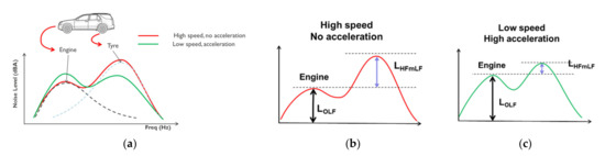
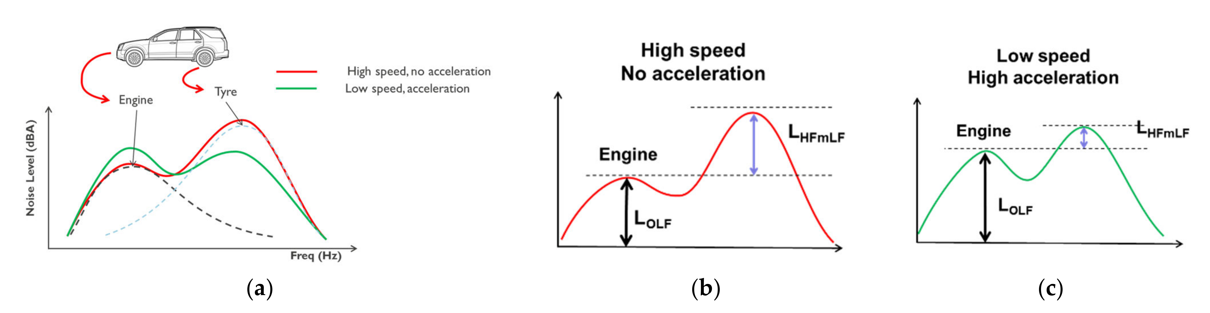
Figure 1.
(a) Visualization of the spectral content of engine and tyre noise for two situations, high and low speed. (b) The two noise parameters, engine noise and cruising noise for a high-speed traffic situation. (c) The two noise parameters for a low-speed traffic situation with acceleration.
The definition of two new noise parameters enabled the assessment of the local traffic dynamics of the vehicle flow from a single spectral noise measurement [9]. The engine noise (OLF) aggregates the low-frequency noise between 100 and 200 Hz (Figure 1b,c). The engine noise correlates with the amount of traffic and the engine throttle. In the model, it is the main parameter, included as magnitude. The second parameter—cruising noise (HFmLF)—is derived from both the engine noise and the rolling noise; more specifically, as the difference between the high-frequency noise (1000 Hz to 2000 Hz) and the engine noise. It indicates the relative contribution of the rolling noise in the overall noise spectrum.
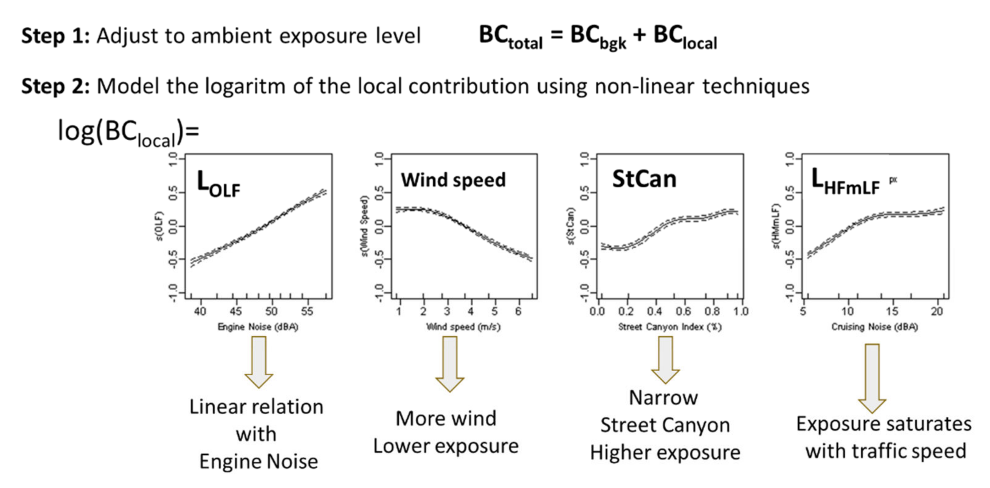
The resulting instantaneous model required a correction for the ambient concentration of the black carbon exposure of the cyclists, but the main short-term variability is explained by a combination of engine noise, wind speed, cruising noise and the street canyon property (see Figure 2). The technique was applied on several occasions, resulting in similar models for Bangalore, India and New York (USA) [12,13]. The main feature of the methodology is the potential to disentangle the traffic dynamics from the meteorological condition, including the ambient concentrations and the fact that the traffic and traffic dynamics can be quantified by unattended noise measurements only. The meteorological bias and the seasonal bias in the air pollution assessments can be resolved to estimate route-specific exposure for both the specific meteorological conditions and for yearly averages [14]. On a different occasion, the trip-by-trip variation in an air pollution-only project was retroactively predicted by measuring the cyclist’s noise exposure on the designed routes two-and-a-half years after the air pollution campaign, resulting in a correlation of 0.75 and higher [15]. Overall, this methodology has proven to be robust and efficient.
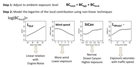
Figure 2.
The cyclist black carbon prediction model is based on the engine noise, wind speed, cruising noise and street canyon index.
In May 2011, completely independent of the work described in the prior sections, the Environmental Research Bureau of the province of Limburg (ERBLimb, the Netherlands) measured ambient levels of a wide range of air pollutants close to a highway and included spectral noise in the measurement campaign [16]. In the resulting report, only NO and UFP were found to be marginally correlating with noise (in LAeq). The correlation methods in this publication did not include insights into the short-term variability and potential of retrieving the traffic dynamics from the noise measurements. The basic aim of that measurement campaign was to compare a wide variety of air pollution equipment. In the publications listed in the previous sections, only black carbon and UFP were subject to the models, and the correlation was evaluated in most cases in a mobile context only. This dataset has the potential to evaluate the methodology for a wide range of air pollutants and for different types of equipment. The aim of this publication is to test the applicability of the methodology with different air pollutants in a fixed monitoring setting, thus focusing on temporal variables instead of spatial variables. The available data also includes traffic data on the highway. Three sets of evaluations will be included in this manuscript: (1) the relation between traffic and noise, (2) the relation between traffic and air pollution, and (3) the relation between noise and air pollution. The resulting models will be ranked. The differences in the models will be related to the physical and chemical properties of the various air pollutants.
2. Materials and Methods
2.1. Measurement Campaign
No new measurements were performed for this publication. Two measurement sessions were held in 2011 in the period from May 11th at 12:00 until May 30th, 8:00, and the second session took place from October 21st at 12:00 until December 8th, 8:00. The second session was largely disturbed due to work on the highway and was therefore excluded from this evaluation. The location is an air quality station in the Province of Limburg, at the eastern side of the entrance of the A2 motorway at Maastricht, Netherlands (elevation 53 m ASL, latitude 50°50′45″ N, longitude 5°42′48″ E). The distance to the road axis is about 30 m. There are no buildings within a close distance of the measurement location. The A2 has two double driving lanes. The traffic intensity is generally about 50,000 per day; heavier traffic is about 8000 per day. The local speed limit is 50 km/h in approaching a traffic light. There is an open area in front of the station of about 80 m until a five stories high (15 m) building of about 110 m in length, east of the motorway in a southwestern direction. Lower buildings are in other directions at about 50 m distance from the station. Around the station, there is some vegetation, which is mostly trees. This situation is not typical for a normal highway speed limit of 50 km/hour and the proximity of the traffic light. In practice, it is a very high-density road in an urban context. Shortly after this measurement campaign was performed, this urban highway was redesigned and was largely transformed into a tunnel. The measured situation does not match the current online maps. The visual representation is available in [16].
2.2. Air Pollution Measurements
The following air pollutants were measured: PM10 (BAM METOne, Province of Limburg), NO, NO2, NOX (Teledyne API200), PM fractions (31 classes Grimm 180) and UFP (8.7–846 nm SMPS). The SMPS size fractions are grouped into eight classes: <20 nm, 20 to 30 nm, 30 to 50 nm, 50 to 70 nm, 70 to 100 nm, 100 to 200 nm, 200 to 500 nm and 500 to 850 nm [16]. Additional information on the measurements can be found in [16].
2.3. Noise Pollution Measurements
The noise measurement was performed with Type1 noise equipment, including spectral content, but the original data in third-octave bands are not available. The microphone was positioned at a height of 3 m. Only six parameters are available in the dataset: the equivalent A-weighted noise level LAeq,1h and the median value of the 1 s values LAeqL50; the unweighted matching values LZeq and LZeqL50 and the octave band values: Leq125Hz and Leq2kHz. LAeqL50 is the median value of the LAeq,1sec values by the hour. The difference between LAeq and LA50 is an indication of the eventfulness of the noise time series.
The engine noise OLF in the original model is the sum of four one-third-octave bands 100, 125, 160 and 200 Hz, including an A-weighting, while Leq125Hz corresponds to the sum of the 100, 125, 160 Hz in unweighted third-octave bands [12]. The mismatch for the high-frequency component is larger. The high-frequency ‘rolling noise’ contribution OHF is the sum of 1000, 1250, 1600 and 2000 Hz A-weighted third-octave bands, in the data; only the Leq2kHz unweighted octave band is available, which is the sum of the 1600, 2000 and 2500 Hz third-octave bands. As a result, the noise parameters defined in the prior work are not available and cannot be calculated from the available information. Two options remain: the use of the data ‘as is’ or adjusting the available data by estimating a correction to fit the original definition. We chose not to adjust the measurement data for the frequency content, however, we applied the A-weighting to the available octave band data. We treated the A-weighted octave band 125 Hz (−16.2 dB), as a good estimate for OLF and the A-weighted octave band 2 kHz (+1.2 dB) minus OLF as a valid estimate for HFmLF. These corrections are linear and do not affect the models as such. The A-weighted correction only aligns the magnitude of the measurement data towards the original definition. Unweighted third-octave bands become, at lower frequencies, larger than the LAeq values. The original decision to present the parameters in an A-weighted format enabled us to present the OLF and OHF parameters as subsets of the LAeq in communication with scientists without acoustic backgrounds. Despite the discussed divergence, the available noise data is close enough to the original definition to evaluate the methodology. It is important to note, however, that absolute values cannot be compared across the different measurement campaigns for other reasons than the mismatch in the measurement data.
In Figure 3, the diurnal patterns of the noise parameters are visualized. The diurnal pattern of OLF shows a larger diurnal variation compared to LAeq (15 dB versus 10 dB). The interquartile range of OLF is larger during the early morning compared to LAeq and OHF. The difference between LAeq and LA50 is shown to illustrate the changing noise situation during the night. When those parameters differ, the noise time series becomes eventful; single vehicles can be detected as separate events. The equivalent acoustical energy LAeq is very sensitive to single events with high maximum values. LAeq is not very sensitive to short quiet periods, while LA50 is sensitive to those quiet periods.
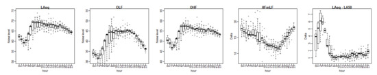
Figure 3.
Diurnal patterns of the noise parameters: LAeq, OLF, OHF, HFmLF and the difference between LAeq and LA50.
2.4. Traffic and Meteorological Data
The hourly traffic data was available by direction of the highway and detailed into three vehicle categories: cars, light freight and heavy freight (trucks). After preliminary evaluation, the traffic data was aggregated into two variables: the cars (CAR) and the sum of light freight (LV) and the heavy freight (HV) over both directions, referred to as LVHV. This choice matches the most typical vehicle categories in third-party traffic data. The definition of vehicle categories can change by third-party data suppliers. The meteorological data were retrieved from in situ meteorological stations after validation with meteorological data from an official station of the KNMI (Royal Dutch Meteorological Institute) [16].
2.5. Modeling Approach
Generalized additive models (GAMs) are regression models where smoothing splines are used instead of linear coefficients for the covariates. This approach is particularly effective for handling the complex nonlinearity associated with air pollution research [15,16]. Smooth functions are developed through automatic smoothing parameter selection using penalized regression splines, which optimize the fit and try to minimize the number of dimensions in the model. The main advantage of GAM modeling is the possibility of adjusting for nonlinear relationships between the covariate and the outcome. The analysis was performed in the R environment for statistical computing with the package ‘mgcv’ [17]. This technique is used frequently to analyse similar problems [18,19,20].
To evaluate a GAM model, the F-values and p-values, the ‘deviance explained’ and the AIC are the relevant parameters. The p-value is converted into categories, matching the strength of the parameter. In the remainder of this manuscript, the same principle is included, using a dot for marginal significance, and one to three stars for increasing significance. The F-value is the best parameter for comparing the relative strength of the covariates in the model. Note, however, that these values cannot be compared directly when the underlying dataset or selected covariates differ. The ‘deviance explained’ and the Akaike information criterion (AIC) is the most relevant parameter to compare models. The physical behavior of the model for the different covariates can be derived from the spline plots. In the spline plots, the full line is the actual spline function, the dotted lines are the confidence intervals on the splines. GAM models include a prediction function that simply adds the corrections—visually presented by the splines—for the given set of covariates plus the intercept of the model. In this publication, the detailed information on the GAM models extensively proceeded in the tables. The matching figures focus on the visual representations of the splines. Evaluating the functionality and relevance of the GAM models requires both sets of information. The linearity of a covariate spline is the most relevant information to understand the predictive potential of the model. Nonlinear splines indicate more complex relations. GAMs can include interactions between variables, but this type of modeling is not required for the aims of this publication. High ‘deviance explained’ means that there is a strong explanatory power of the covariates for the selected outcome and that the data is ‘not noisy’.
3. Results
The results will be presented in three sections. In the first section, the relation between de-noise measurements and the traffic data is evaluated. The purpose of this section is to illustrate the validity of the relation between the traffic data and the noise measurements. It also supports the decision to select the noise parameter used in the ‘noise-as-a-traffic-proxy’ methodology. In the second section, the air pollution is modeled with the traffic data. This acts as a set of reference models to compare with the noise-based air pollutant models. In the third section, the air pollution is modeled using the noise parameters. Some discrepancies are detected in the UFP models and this is investigated in more detail in the fourth section. The comparison of the models is presented in the fifth section.
3.1. Traffic-Noise Models
3.1.1. Basic Traffic-Noise Models
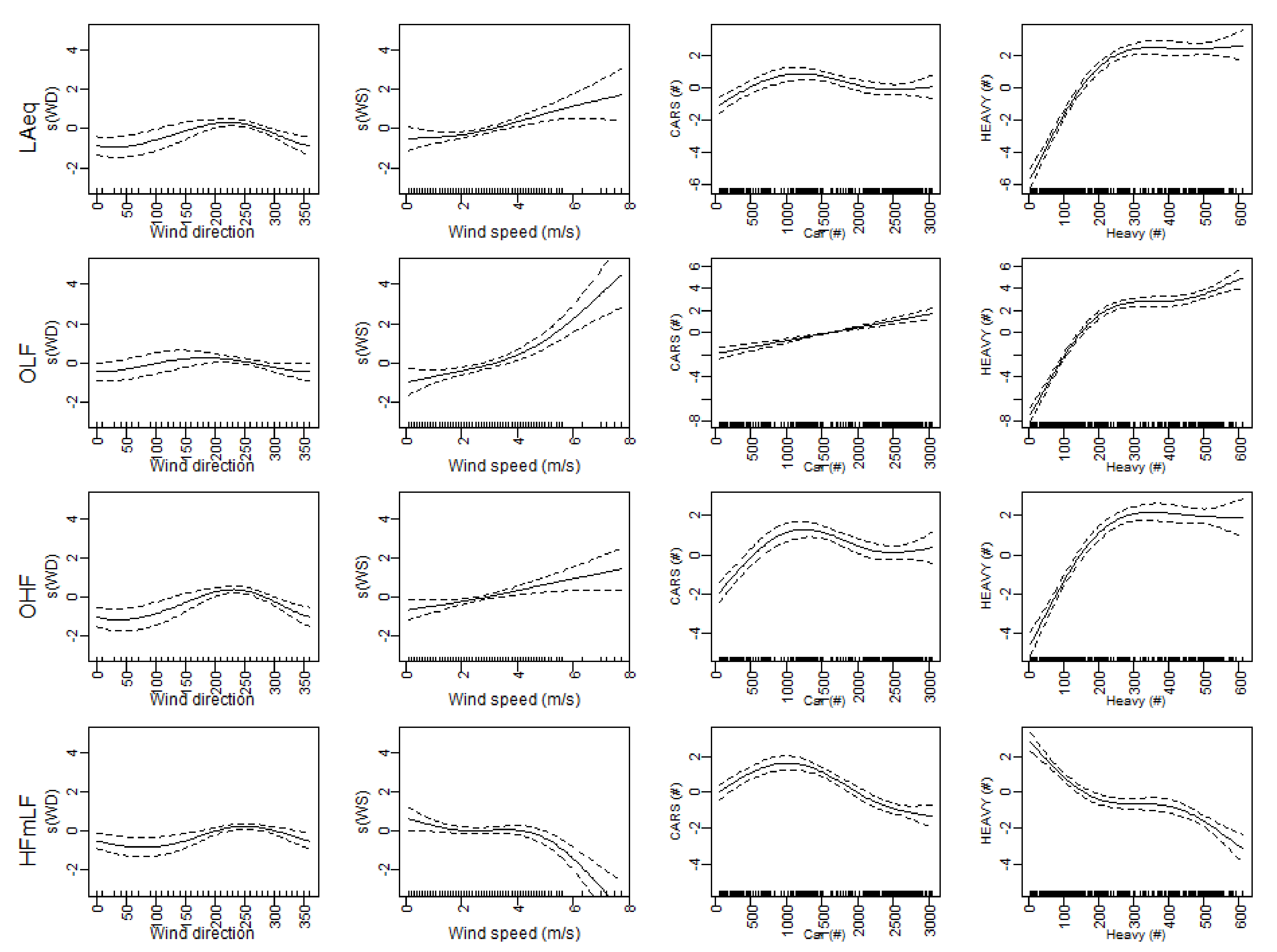
The GAM models are constructed in two variants, a basic version with only the wind speed and wind direction as external covariates and a meteorological extended version, including temperature and humidity. In Figure 4, the four basic traffic models for LAeq, OLF, OHF and HFmLF are presented. In this section, the OHF is included to illustrate the functionality of the HFmLF noise parameter. The only model with a positive correlation with both the number of cars and trucks is the engine noise OLF. The contribution of heavy vehicles saturates at relatively low levels (250 vehicles per hour). The relation between car traffic is low to non-existing for both LAeq and OHF; the heavy traffic showed a positive relation but saturates from 200 vehicles per hour. The behavior of OHF is very similar and indicates that the higher frequencies in the spectrum determine the LAeq value.
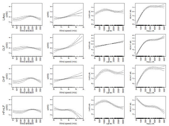
Figure 4.
Four sets of GAM models for the noise parameters: LAeq, OLF, OHF and HFmLF.
In contrast, the HFmLF does relate to a physical property of the traffic near the measurement location. From about 1000 cars per hour and for heavy vehicles per hour over the whole traffic range, HFmLF decays. The relative contribution of the high frequencies drops with high traffic volumes and expresses the reduction in the rolling noise, which relates to a reduction in the typical speed of the vehicle flow. It is an indication of traffic jams with many starts and stops, thus a lot of engine noise, but at very low average speeds.
At very low traffic volumes, the LAeq noise level is still high and is dominated by single events of vehicles at free-flow speed, and night-time values still exceed 58 dBA (see Figure 3). The LAeq and OHF parameters are strongly affected by single events during the night and when traffic volumes are low, other noise sources, such as background noise from the city and nearby industry, determined the lowest noise values.
The intermediate conclusion is that the engine-related noise OLF is the main covariate linking traffic to noise. At high values, the relative contribution of the rolling noise to the overall noise level drops. This illustrates the speed reduction in the traffic flow for higher traffic volumes. Remember, the speed limit on this urban highway is 50 km/h. Even at this relatively low speed, the cruising noise covariate (HFmLF) is sensitive to the speed. In the vicinity of roads with higher speeds, this covariate will reach higher values [9,12,13]. The details of the models are presented in Table 1. The OLF model outperforms the LAeq model, with a ‘deviance explained’ of 0.88 versus 0.78.

Table 1.
Summary of the GAM models for the noise parameters: LAeq and OLF, with and without temperature and relative humidity.
The HFmLF displays the expected behavior for prior work; it acts as a vehicle flow speed indicator. No average speeds are available from the third-party data to confirm this, but this relation is established in the field of acoustics. The OLF model is less affected by wind direction compared to the LAeq model.
3.1.2. Meteorology Extended Traffic-Noise Models
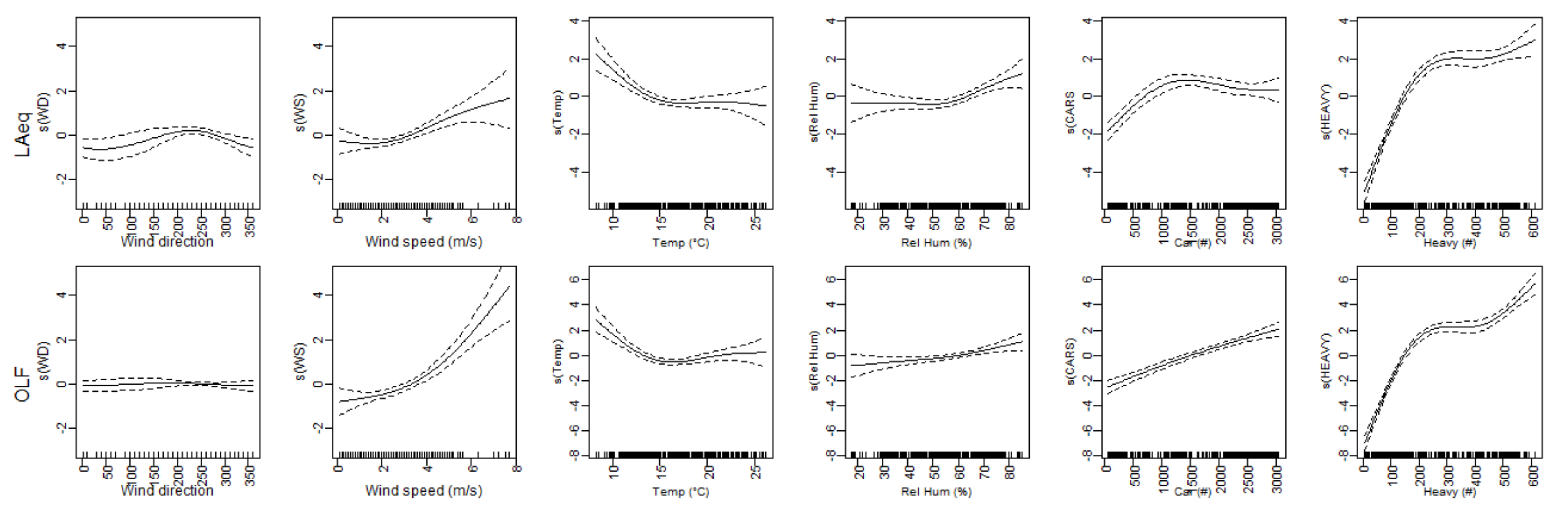
The noise measurements were affected by the meteorological conditions, wind speed, wind direction, humidity, the temperature of the air and the road surface, stability of the atmosphere and others. Evaluating the impact of these variables is—despite the short distance to the source—still relevant. In the basic model, the wind speed and wind direction are included. In this section, the impact of temperature and humidity is included in the models. Only two models are retained in this section, ‘LAeq_meteo’ and ‘OLF_meteo’. To compare the two approaches, the details of the GAM model are presented in Table 1 and the resulting splines in Figure 5. Lower temperatures result in higher values. This is an established acoustic phenomenon related to various physical properties of vehicle noise emission (rubber becomes softer and produces less noise, the same issue applies to road surfaces). The most relevant in this context is the harder rubber of the tyres at colder temperatures, resulting in noisier tyre–road surface interactions. The typical value is 1 dB decay per 10 °C [10]. The increase in the noise level with relative humidity is related to the wet road surface; relative humidity acts as a proxy for rain. Tyre–road interactions emit more high-frequency noise due to the splashing of the water, but a film of water will also increase the acoustical properties of the road surface at low frequencies. The effect of a wet road surface is stronger in LAeq than in OLF. Adding the additional meteorological variables does not affect the comparison. Note, however, that temperature expresses a similar diurnal pattern as the traffic densities and is therefore partially competing with the traffic variables. This effect is stronger in the LAeq model compared to the OLF model, which supports the OLF approach even further.
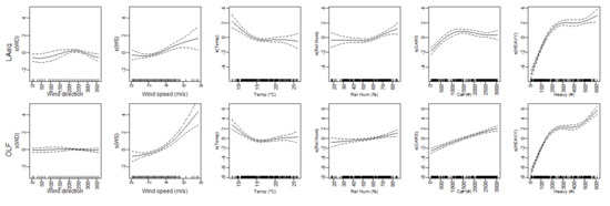
Figure 5.
Two GAM models for the noise parameters: LAeq, OLF, including temperature and relative humidity.
The extended OLF model outperforms the LAeq model, with the ‘deviance explained’ respectively 0.90 and 0.83. The decision to use OLF as the main noise-as-a-proxy is supported by the linear spline for the number of cars and the monotone spline for the number of heavy vehicles. The LAeq model still includes the reduction in noise levels for high numbers of cars since it is sensitive to the speed of the vehicle flow. This information is available in the HFmLF covariate. The established behavior of OLF and HFmLF in prior work is hereby validated in the dataset used in this manuscript: the engine-related noise is a stronger predictor of the total traffic volume compared to LAeq. This feature identifies why air pollution and noise exposure comparison without including the spectral content of noise are sensitive to failure. The traffic dynamics affect the relation between traffic volumes and LAeq significantly. LAeq is, by consequence, not the best indicator to relate traffic volumes to air pollution data.
3.2. Traffic-Air Pollution Models
3.2.1. Basic Traffic-Air Pollution Models
The basic air pollution models match the structure of the noise-traffic models with four covariates: wind direction, wind speed, the number of cars and heavy traffic. The results of the models are presented in Table 2 (bottom half). Figure 6 shows the splines for a relevant selection of the models.
Table 2.
Summary of the GAM models for the noise parameters: LAeq and OLF, with and without temperature and relative humidity.
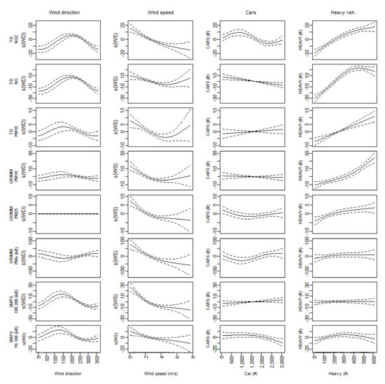
Figure 6.
Selection of the basic traffic-air pollution GAM models: NO2, NO, PM10 (BAM); PM10, PM2.5 and PMx (GRIMM); UFP count 100–200 nm and 70–100 nm (SMPS).
The ‘deviance explained’ ranges from 0.07 to 0.55. The relation between air pollution and traffic is more complex compared to noise. The strongest models are NOx, NO and NO2—the pollutants with a direct relation to combustion. The particulate matter with the larger size fraction is the next set: PM10 and the larger bins of the SMPS. The smallest size fractions result in the lowest ‘deviance explained’. Note, however, that the calculated result for GRIMM PM10 outperforms the BAM PM10. The strongest traffic variable is the heavy traffic, but only the NO, NO2 and NOx show strong monotone relations with traffic volumes (not all shown). For the PM10 fractions, the monotone relation also exists. The form of the spline for the number of cars is highly variable. Most are not significant, but in some cases, a reduction in concentration is found for the highest traffic volumes. This might relate to the reduced emissions during traffic jams. For the UFP parameters, the picture is more complex. The slopes of the traffic variables are non-existing or show a maximum for average traffic volumes. This might relate to the reduced emissions during traffic jams as well.
The strongest aberration in the UFP and PM10 models is the effect of wind direction. These splines show higher levels for UFP for the southeast wind direction, while the main local source is in the southwest, clearly depicted in the NO models. This suggests different sources or different lifetime behavior. It is known that the smallest particulate matter is scavenged efficiently when larger amounts of larger particles are available. At high traffic volumes, the small particles are removed. When the wind direction feeds the measurement location with less dense traffic, the smallest particles reach the measurement location before being scavenged. This can explain the different behavior of the UFP fractions. The smallest UFP fractions do correlate with traffic, potentially expressing the delayed formation of the smallest particles.
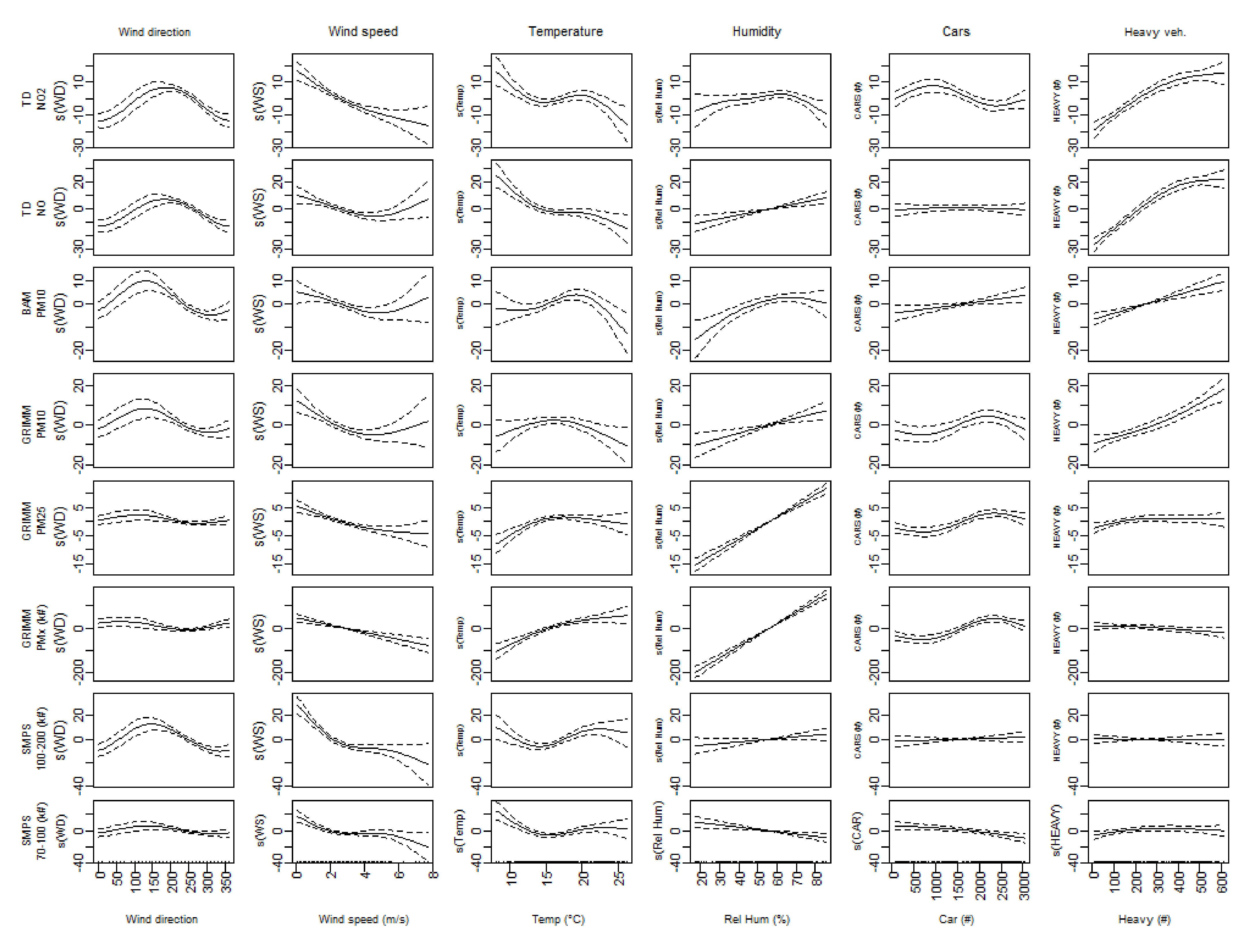
3.2.2. Meteorology Extended Traffic Air Pollution Models
In this section, the basic air pollution models are extended with temperature and relative humidity. The results of the models are presented in Table 2 (top half). Figure 7 shows the splines for a relevant selection of the models. Including the additional meteorological variables improves the models significantly. The ‘deviance explained’ range shifts from 0.07–0.55 to 0.22–0.66 when including the meteorology. The temperature covariate is highly significant in most models, but for the intermediate PM fractions, PM2.5, PM1, PMx and 200–500 nm, the relative humidity is the dominant covariate. For the smallest fraction, both covariates have a similar significance.
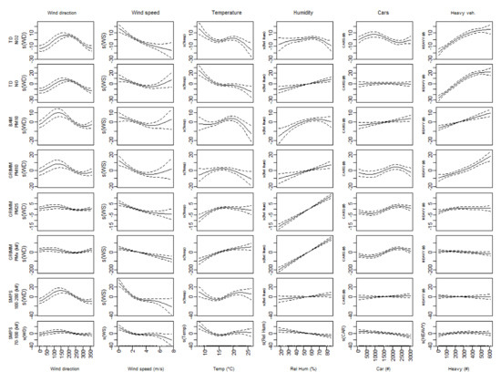
Figure 7.
Selection of the extended traffic-air pollution GAM models that include temperature and relative humidity: NO2, NO, PM10 (BAM); PM10, PM2.5 and PMx (GRIMM); UFP count 100–200 nm and 70–100 nm (SMPS).
The strongest models are again NOx, NO and NO2. The features detected in the basic models are enhanced after the inclusion of temperature and relative humidity: stronger slopes for heavy vehicles and a reduction for high car volume related to traffic jams. The increase in concentrations during the lowest temperatures relates to the stable atmosphere during the night-time period, similar and correlating to the higher levels under low wind speed. The relative strength of the heavy vehicle covariate in the models is increased, but the significance of the car covariate drops slightly in the NO2 model. NO is not correlating with the number of cars.
The larger size fraction particulate matter PM10 and 500–850 nm shows similar behavior as the NO models but is less expressed. The ‘deviance explained’ is about half of the NO models; the variability is less explained by traffic. The smallest size fractions result in the lowest ‘deviance explained’ and the correlation with traffic is variable, sometimes the heavy vehicle covariate is significant, and sometimes it is the car variable. No clear relation can be seen in the relevant splines. Adding the meteorological variables does not reveal a direct source-based contribution except for the smallest UFP fractions, where an inverse relationship with the car traffic is visible.
3.3. Noise-Air Pollution Models
3.3.1. Basic Noise-Air Pollution Models
The basic noise-air pollution models match the structure of the traffic-air models but replace the number of cars and heavy traffic with the two predefined noise covariates: OLF and HFmLF. The results of the models are presented in Table 3 (bottom half). Figure 8 shows the splines for a relevant selection of the models. In this approach, the OLF covariate aggregated all traffic density information into a single covariate, while the HFmLF added value by detecting the speed of the vehicle flow.
Table 3.
Summary of the GAM models for the noise parameters: OLF and HFmLF, with and without temperature and relative humidity.
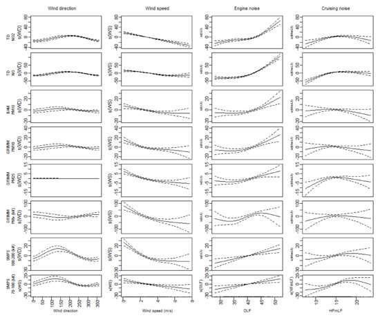
Figure 8.
Selection of the basic noise-air pollution GAM models: NO2, NO, PM10 (BAM); PM10, PM2.5 and PMx (GRIMM); UFP count 100–200 nm and 70–100 nm (SMPS).
The range of the ‘deviance explained’ shifts in the basic traffic-air models from 0.07–0.55 to 0.06–0.70. The NO, NO2 and NOx show the highest ‘deviance explained’. In the splines, the expected behavior is visible for all air pollutants, with an upward slope for the engine-related noise OLF and saturation or a downward slope for the cruising noise covariate HFmLF. In the models for the smaller size fraction, the significance of the OLF covariate drops (PM1, PMx, 50–70 nm and 30–50 nm). The fractions below 30 nm do show a positive correlation with traffic (not shown). Similar variability in model performance is seen in the basic noise-air models.
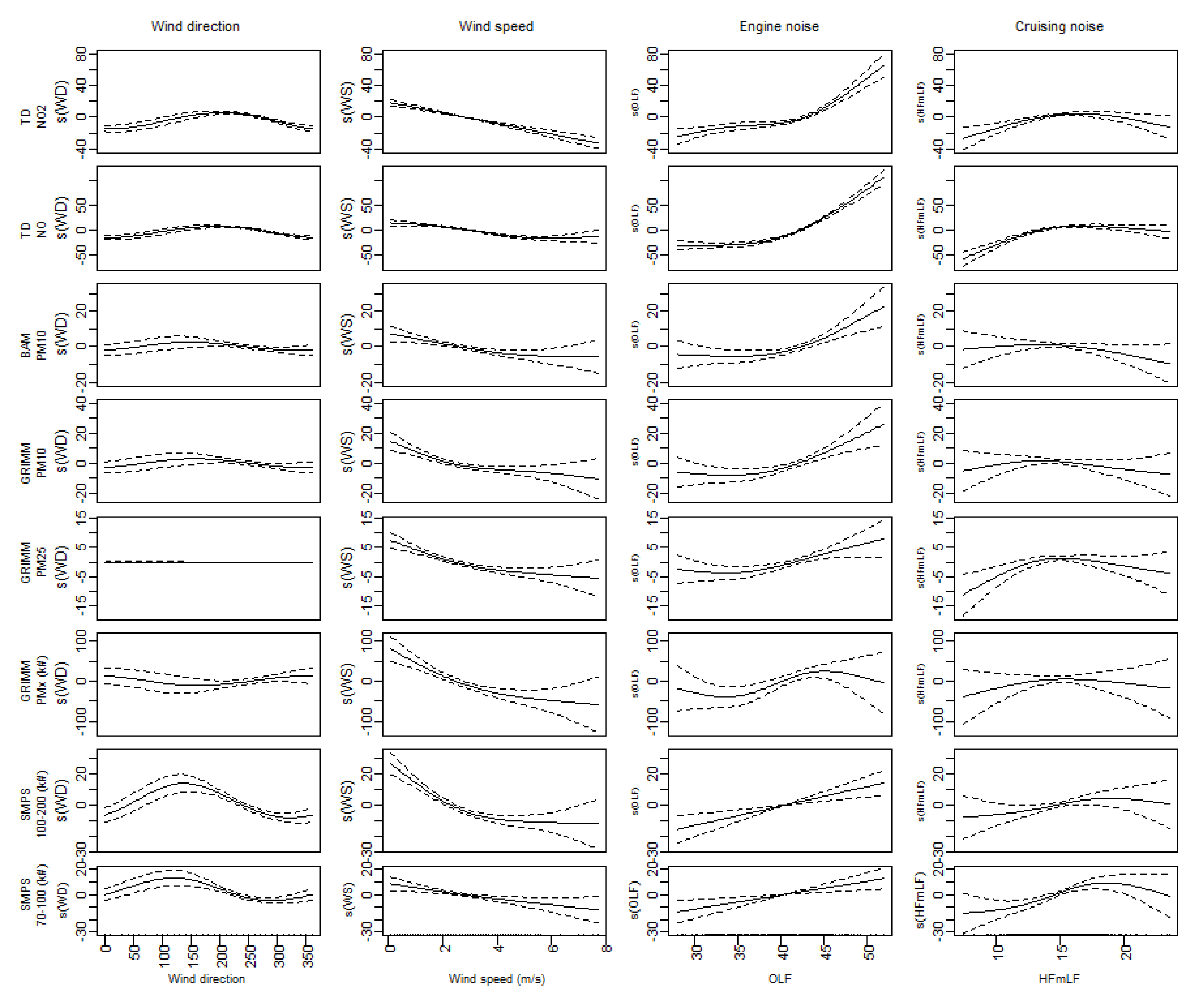
3.3.2. Meteorology Extended Noise-Air Pollution Models
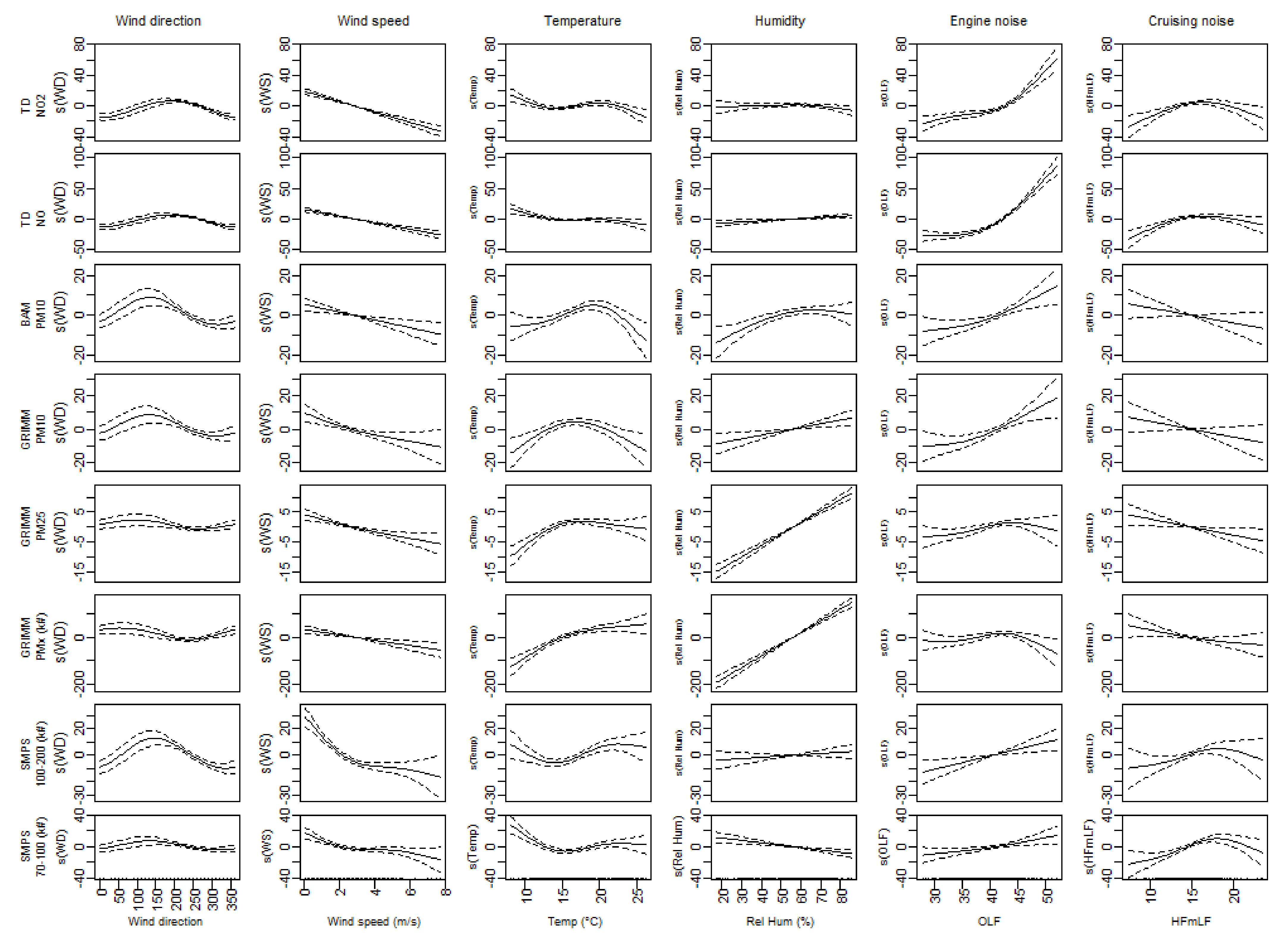
In this section, the basic noise-air pollution models are extended with temperature and relative humidity. The results of the models are presented in Table 3 (top half). Figure 9 shows the splines for a relevant selection of the models. The range of the ‘deviance explained’ shifts from 0.22–0.66 to 0.21–0.73. Similar behavior for the inclusion of the meteorological variables is visible. The NO, NO2 and NOx models show higher ‘deviance explained’ and the confidence intervals of the splines are reduced. Adding the meteorological variables strengthens the models and supports the engine noise and cruising noise as valid traffic proxies.
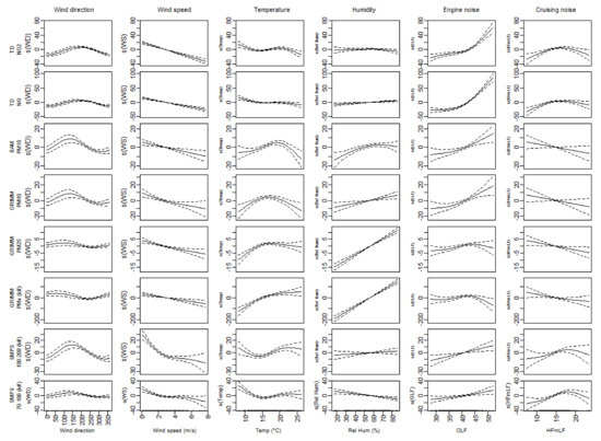
Figure 9.
Selection of the extended noise-air pollution GAM models that include temperature and relative humidity: NO2, NO, PM10 (BAM); PM10, PM2.5 and PMx (GRIMM); UFP count 100–200 nm and 70–100 nm (SMPS).
The PM models behave differently than the NO models and show similar changes as the extended traffic-air models. The relative humidity becomes the most dominant covariant for the medium size fractions (PM2.5, PM1) and the most important covariate, sometimes slightly reducing the significance of the OLF covariate. The smallest UFP size fraction shows a poor correlation with the engine-related noise.
3.4. Comparison of the Noise and Traffic Models for Air Pollution
In Table 4, the comparison of the models is presented. The evaluation is based on the ‘deviance explained’ and the AIC. The table is organized to compare the effect of replacing the traffic variables with the noise-as-a-proxy variables for both the basic and extended models. The NO, NOx and NO2 models result in a systematic improvement of the models in all variants, sometimes with a rise of 10% to 15% in the ‘deviance explained’. For the NO2 models, the increase is the lowest. The PM10 models show a systematic decrease in the model quality, especially for the data from the GRIMM. This does not discredit the approach since PM10 is very sensitive to variability in large-scale changes in the ambient concentrations. The missing background correction might be at the origin of this decrease. For PM2.5, the basic model increases, and the extended model decreases. Again, this can be related to the missing correction for the ambient concentrations.
Table 4.
Comparison of the traffic and noise models in two variants, base and meteo extended. Green indicates improvement with the noise-as-a-proxy approach, red is failing, and orange is undetermined.
The variation due to the ambient concentration is not independent of the meteorological variables (wind speed, temperature, wind direction, etc.). Including the temperature and humidity results in an indirect correction for the behavior of the ambient concentration. This phenomenon of overfitting the data by including a set of entangled variables was illustrated extensively in the mobile measurement performed in New York [13]. The difference between the base models and the meteo-included models is very stable, indicating that overfitting due to the interactions between the meteorological variables is not an issue in this dataset.
The UFP count from the GRIMM behaves in the same way as the calculated size fractions, and this behavior does not align with the data from the SMPS. For the smaller size fraction, the results vary; the bins between 70 and 500 nm slightly increase, while the bins between 20 and 70 decrease slightly. In general, the noise attributes perform at least as well as the traffic variables, except for PM10. For UFP, the conclusion is mixed. A relation with noise emerges, however, the ‘deviance explained’ is low.
3.5. Different Behavior of PM and UFP Fractions
For the larger size fraction PM2.5 and PM10, evidence shows large contributions of non-traffic sources and significant impacts of long-distance transport. The low performance of the methodology for these components is expected. In the prior analysis, levels of PM10 and NOx of both air quality stations A2 Maastricht and Asterstraat-Geleen were compared to test consistency. Historical data from these two stations showed that both PM10 and NOx levels mirror a common background contribution from southwestern regions controlled by dominant southwestern winds in this region [16]. The low performance for UFP was not expected; the high-resolution time series in prior work resulted in a stronger correlation compared to the data collection under evaluation [12,13]. The different behavior of the UFP fractions is expressed for both the traffic and the spectral noise parameters. The unexpected behavior of the wind direction requires additional analysis to identify the origin of this discrepancy. The first option is the possibility of non-road traffic sources, and the second option is the potentially different behavior of UFP compared to the direct combustion-related gaseous pollutants.
Data exploration showed that the highest values occur during the evening, early night and a systematic early morning peak, occurring before the morning rush hour. The highest values occur during upwind conditions in the evening hours. These patterns are not dominated by a typical road traffic diurnal pattern. An alternative source is a possibility. Near Maastricht, a small airport (ICAO code MAA) with approximately 10,000 movements a year is located to the north of Maastricht. Aircraft are known to emit significant amounts of UFP. This airport is a source of UFP, potentially affecting the measurement dataset under investigation [21,22,23,24]. The measurement location is positioned between the arrival pathway under atypical operational conditions (northeast winds) and the departure pathways during normal operation conditions (southwest winds). The arrival pathway coincides partially with the downwind conditions for the urban highway, but the departure pathway is entirely under upwind conditions for the urban highway. The departures are known to emit significantly higher levels of UFP compared to the arrivals, in line with the operational modus of the aircraft engines [21]. The peak UFP levels occur in the evening, early night and early morning. This behavior cannot be uniquely linked to aircraft movements since the airport is not operating during the nighttime and early morning. Although possible, in this specific setting, the high UFP level is mostly not related to the airport. The two main arguments are the low number of operations at the airport and the mismatch in diurnal patterns of exposure and operations. An alternative explanation is required.
To investigate the UFP diurnal pattern in more detail, the GAM models are extended with an hour of the day covariate. Adding the hour of the day will reveal the discrepancy between the hourly traffic covariates and the diurnal pattern of the UFP.
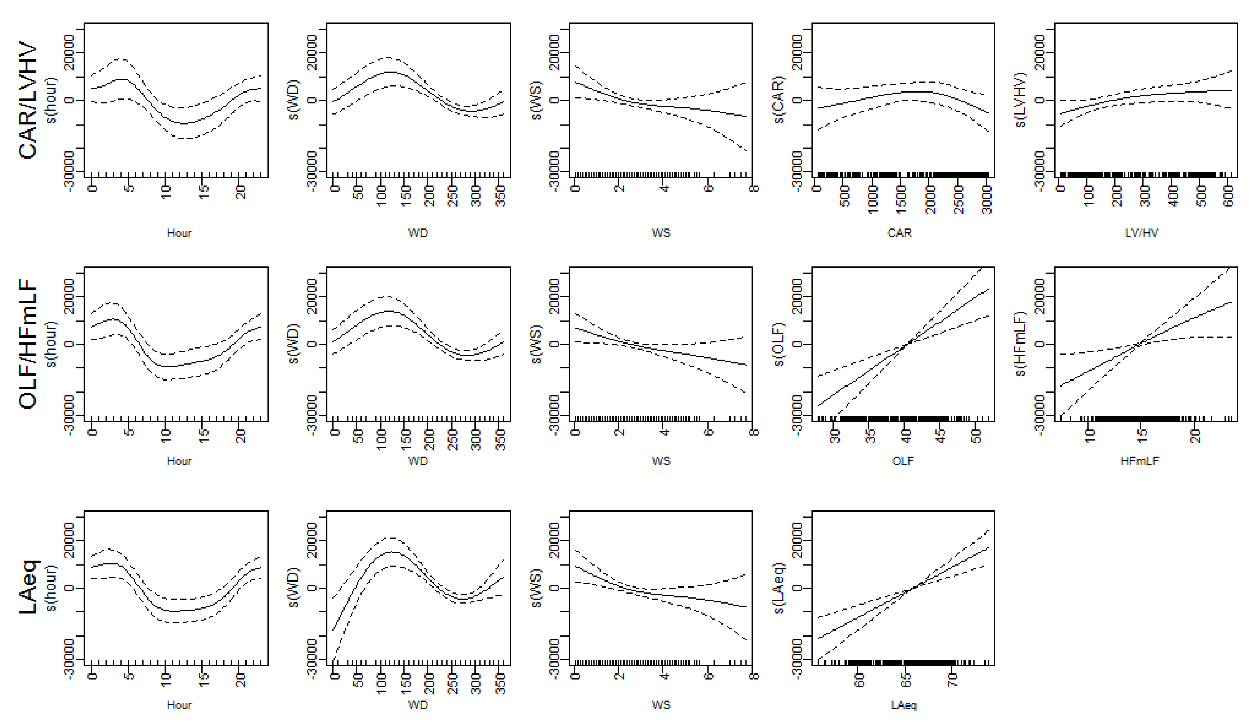
In Figure 10, the GAM models for the SMPS size fraction 70 to 100 nm, including the hour of the day covariate, are presented for three variants of traffic variables: the traffic data covariates (top row), the spectral noise covariates (mid-row) and LAeq as a single traffic attribute (bottom row). The matching GAM evaluation is available in Table 5. The splines of the SMPS 70 to 100 show a strong inverted diurnal pattern for all models. This mismatch with traffic volumes suggests a different behavior compared to the air pollution components, with a direct relation to the combustion processes. The traffic data (CAR and LVHV) is not significant in the GAM model, while OLF and HFmLF are significant. The behavior of HFmLF is aberrant; it shows a linear relation with UFP. This means that the UFP levels are not reduced at higher speeds—the typical behavior of the other combustion-related air pollutants. This behavior means that the spectral content of the noise is not adding value. This is illustrated in the LAeq model, where—after including the hour of the day as a covariate—a single traffic related covariate results in a linear relation with UFP. This model, with only four parameters, has a higher ‘deviance explained’ compared to the two other five covariant models.
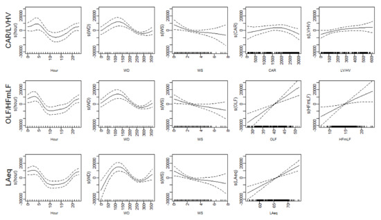
Figure 10.
GAM models for the SMPS size fraction 70 to 100 nm, including the hour of the day as a covariate for three models: the traffic parameters (top), the spectral noise parameters (mid) and LAeq (bottom).
Table 5.
Summary of the GAM models one size fraction (SMPS 70 to 100 nm), including the hour of the day as a covariate for the traffic parameters, the spectral noise parameters and LAeq.
The spectral noise covariates are adding additional information on traffic dynamics, but the traffic dynamics doesn’t affect the UFP levels. LAeq detects traffic, and, as such, is less correlated with the traffic volumes (see Section 3.1) but it is the strongest traffic variable for the UFP size fractions. The UFP concentration is predominantly determined by particle dynamics, presumably by coagulation when larger size fractions are available in the ambient air [20]. High UFP size fractions require relatively clean air and ‘some’ traffic. In heavy traffic, the smaller particles are scavenged by the larger particles. The spline of the hour of day covariate can be interpreted as a ‘UFP survival’ function; high during low traffic, low during high traffic. This aligns with the highest peaks when upwind conditions for the urban highway exist. Under these circumstances, the measurement location is more affected by roads with less traffic. A contribution from single events of aircraft departures during these northeast wind conditions cannot be excluded, however, this is not considered dominant.
4. Discussion
4.1. Limitations
It is evident that this retrospective analysis has its limitations. One main difference with the original methodology is the lack of ambient exposure to the available air pollutants. The ambient concentration is mainly determined by large-distance transport and large-scale meteorological variations. Additionally, the measurement period was only one month in spring. The ambient concentrations show strong seasonal effects which are—by design—not included in the data. Prior knowledge does suggest that even day-to-day changes in ambient conditions affect the models. Especially for PM10 and PM2.5, we can expect that a correction for the ambient concentration might improve the presented models. In a nearby air pollution measurement location, installed for dedicated assessment of a local industrial facility in an area with little local traffic, PM10 is measured. This data is used as a small test of including an ambient correction. It revealed that correcting for the ambient levels results in a GAM model with OLF as the only significant covariate. The resulting ‘deviance explained’ is 0.11. An effect of the urban highway after adjusting for the ambient concentration is detectable in the background-adjusted model. The experiment was designed to exclude seasonal patterns. This design feature reduces the relevance of the background correction. Furthermore, this background correction could not be pursued for the other pollutants and is therefore not included in this manuscript. An additional argument to perform this analysis without ambient level correction is the very short distance to a major source. It is reasonable to expect, however, that the local urban highway is the dominant source.
Another relevant limitation is the temporal resolution of the data. This evaluation is based on the readily available hourly aggregated data. Traffic flow variation may affect the measurements in a shorter time resolution. Note, however, that the methodology is based on one-second (mobile) measurements, modeled in a temporal resolution of 10 s [9]. A similar evaluation should attempt to perform these analyses in a higher temporal resolution. Higher-resolution data might correlate stronger with the noise covariates. The temporal resolution of one hour is, in the authors’ opinion, the main reason why the correlation with the noise-as-a-proxy method fails. The resolution of the time series does not match the time resolution of the particulate dynamics.
The noise covariates in this evaluation do not align with the original definition—mainly for the HFmLF covariate, which differs significantly from the original approach. The contribution of the rolling noise is the largest in the 1000 Hz band, which is not available in the data. The sensitivity of the restricted HFmLF to the cruising noise variability in this analysis might be significant. These limitations result in the conclusion that this dataset is largely exploited, as is; additional validations should be performed on other and preferable new collected data.
The list of potential influencing external factors on the data is long. The focus of this manuscript is on the short-term variability of traffic volumes and traffic dynamics. Changes in fleets, the impact of regulations, tyres, road types and road quality all affect this relationship; however, most of these influences are long-term temporal trends and/or spatial variables and thus out of the scope of the collected data.
4.2. Behavioral Difference between Air Pollutants
It is clear that the noise-air pollution relationship is complex. For pollutants directly related to the combustion processes, the spectral noise content provides significant added value. For pollutants emitted by various non-traffic sources, the relation to the local noise measurements is inevitably more prone to other spatial and temporal variables. In this evaluation, no background corrections were included. PM2.5 and PM10 are known to be highly sensitive to large-scale variability and long-distance transport and are less correlated with local traffic sources. For PM2.5 and PM10, the noise-as-a-traffic-proxy fails. This is mostly due to the large variety of sources and—by definition—low specificity for combustion-related traffic emissions. Abrasions of tyres and breaks are known to affect the large size fractions of particulate matter as well, but the methods to evaluate this pollution component require a chemical analysis of dust physically collected from samples [25]. As a result, these contributions cannot be assessed in similar temporal resolution to noise and general air pollutants. More advanced experimental setups are necessary to address this non-combustion-related source for PM. Abrasions of tyres and breaks are affected by the definition of the local traffic dynamics. Further research into this area is necessary. Enriching these data collections with spectral noise measurements is potentially insightful.
For UFP, the relation is more highly affected by particle dynamics, presumably by the increased removal when larger size fractions are available in the ambient air. High UFP size fractions require relatively clean air and some traffic. In Section 3.1, OLF shows a higher correlation with the traffic data, while LAeq shows more correlation to small amounts of traffic. For the UFP models, the availability of a little traffic is more important than the traffic volume itself. This feature is captured better with LAeq than with OLF and this is expressed in the UFP models.
4.3. Noise as a Traffic Proxy
It is evident that traffic data is important to building source-based models. Traffic data is scarce, not instantly available and only available in lower temporal resolutions. It is not available for smaller roads. The noise-as-a-proxy covariates provide indirectly measured attributes and include additional information on the speed of the vehicle flow dynamics. The added value is clearly visible in the NO models—not surprisingly, the air pollutants relate directly to the traffic volumes and the traffic dynamics. The presented results are the first direct evidence that the noise-as-a-proxy methodology will work as well for NO2, NO and NOx. Since these types of air pollution measurements are very complex and no equipment is available to assess these pollutants with high temporal resolution in a mobile context, the noise-as-a-proxy method can provide insights. The best way to achieve this is to align other air pollutants with similar properties to NO2, NO and NOx. Black carbon was not included in this study, however, it was a strong candidate to achieve this.
The main feature of the modeling approach, both for traffic and noise-based, is the validity of the source-based models. This allows simulations and predictions. An important topic is the evaluation of interventions, illustrated in [13]. Interventions can be intentional by changing the traffic or fleet composition, but also unintended or even accidental interventions, such as pandemics affecting public life, can be evaluated in a more rigorous way, as short-term changes in traffic density can be collected with measurement equipment. Noise measurements fulfill all requirements. The noise measurements are evidently also relevant for the within discipline evaluations, however, merging and integrating knowledge and data across disciplines should be a priority for many other reasons. The emergence of smart-city initiatives and the related policy support tools are the way of the future. Integrating noise and air pollution into these platforms is a bare necessity.
Author Contributions
Conceptualization, L.D.; methodology, L.D.; software, L.D.; formal analysis, L.D.; investigation, M.S.; resources, M.S.; data curation, M.S.; writing—original draft preparation, L.D.; writing—review and editing, L.D. and M.S.; visualization, L.D. All authors have read and agreed to the published version of the manuscript.
Funding
This research received no external funding.
Institutional Review Board Statement
Not applicable.
Informed Consent Statement
Not applicable.
Data Availability Statement
Not applicable.
Conflicts of Interest
The authors declare no conflict of interest.
References
- Tetreault, L.F.; Perron, S.; Smargiassi, A. Cardiovascular health, traffic-related air pollution and noise: Are associations mutually confounded? A systematic review. Int. J. Public Health 2013, 58, 649–666. [Google Scholar] [CrossRef] [PubMed] [Green Version]
- Allen, R.W.; Davies, H.; Cohen, M.A.; Mallach, G.; Kaufman, J.; Adar, S.D. The spatial relationship between traffic-generated air pollution and noise in 2 US cities. Environ. Res. 2009, 109, 334–342. [Google Scholar] [CrossRef] [Green Version]
- Fecht, D.; Hansell, A.; Morley, D.; Dajnak, D.; Vienneau, D.; Beevers, S.; Toledano, M.B.; Kelly, F.J.; Anderson, H.R.; Gulliver, J. Spatial and temporal associations of road traffic noise and air pollution in London: Implications for epidemiological studies. Environ. Int. 2016, 88, 235–242. [Google Scholar] [CrossRef] [PubMed] [Green Version]
- Davies, H.W.; Vlaanderen, J.J.; Henderson, S.B.; Brauer, M. Correlation between co-exposures to noise and air pollution from traffic sources. Occup. Environ. Med. 2009, 66, 347–350. [Google Scholar] [CrossRef] [PubMed]
- Ross, Z.; Kheirbek, I.; Clougherty, J.E.; Ito, K.; Matte, T.; Markowitz, S.; Eisl, H. Noise, air pollutants and traffic: Continuous measurement and correlation at a high-traffic location in New York City. Environ. Res. 2011, 111, 1054–1063. [Google Scholar] [CrossRef]
- Kim, K.-H.; Ho, D.X.; Brown, R.J.; Oh, J.-M.; Park, C.G.; Ryu, I.C. Some insights into the relationship between urban air pollution and noise levels. Sci. Total Environ. 2012, 424, 271–279. [Google Scholar] [CrossRef] [PubMed]
- Gan, W.Q.; McLean, K.; Brauer, M.; Chiarello, S.A.; Davies, H.W. Modeling population exposure to community noise and air pollution in a large metropolitan area. Environ. Res. 2012, 116, 11–16. [Google Scholar] [CrossRef]
- Kheirbek, I.; Ito, K.; Neitzel, R.; Kim, J.; Johnson, S.; Ross, Z.; Eisl, H.; Matte, T. Spatial variation in environmental noise and air pollution in New York City. J. Urban Health 2014, 91, 415–431. [Google Scholar] [CrossRef] [Green Version]
- Dekoninck, L.; Botteldooren, D.; Panis, L.I. An Instantaneous Spatiotemporal Model to Predict a Bicyclist’s Black Carbon Exposure Based on Mobile Noise Measurements. Atmos. Environ. 2013, 79, 623–631. [Google Scholar] [CrossRef] [Green Version]
- Kephalopoulos, S.; Paviotti, M.; Anfosso-Lédée, F. Common Noise Assessment Methods in Europe (CNOSSOS-EU); EUR 25379 EN; Publications Office of the European Union: Luxembourg, 2012; JRC72550. [Google Scholar] [CrossRef]
- Ntziachristos, L.; Gkatzoflias, D.; Kouridis, C.; Samaras, Z. COPERT: A European road transport emission inventory model. In Information Technologies in Environmental Engineering; Springer: Berlin/Heidelberg, Germany, 2009; pp. 491–504. [Google Scholar] [CrossRef]
- Dekoninck, L.; Botteldooren, D.; Panis, L.I.; Hankey, S.; Jain, G.; Karthik, S.; Marshall, J. Applicability of a noise-based model to estimate in-traffic exposure to black carbon and particle number concentrations in different cultures. Environ. Int. 2015, 74, 89–98. [Google Scholar] [CrossRef] [Green Version]
- Dekoninck, L.; Yang, Q.; Zhao, H.; Ross, J.; Jack, D.; Chillrud, S. An international application of the city-wide mobile noise mapping methodology: Retro-active traffic attribution on a bicycle commuters health study in New York City. In Inter-Noise and Noise-Con Congress and Conference Proceedings; Institute of Noise Control Engineering: Madrid, Spain, 2019; Volume 259, pp. 3265–3276. [Google Scholar]
- Dekoninck, L.; Botteldooren, D.; Panis, L.I. Using city-wide mobile noise assessments to estimate annual exposure to Black Carbon. Environ. Int. 2015, 83, 192–201. [Google Scholar] [CrossRef] [Green Version]
- Dekoninck, L.; Hofman, J. Multi-disciplinary sensing for personal exposure assessments: Quantifying the impact of traffic interventions and meteorological variability. In Proceedings of the e-Forum Acusticum, Lyon, France, 20–24 April 2020; pp. 3085–3090. [Google Scholar]
- Severijnen, M. Relations between Traffic-Generated Nitrogen Oxides, Particulate and Ultrafine Particulate Matter and Noise Characteristics at the A2 Motorway Air Quality Station at Maastricht, the Netherlands; Elsevier: Amsterdam, The Netherlands, 2015. [Google Scholar] [CrossRef]
- Dominici, F.; McDermott, A.; Zeger, S.L.; Samet, J.M. On the use of generalized additive models in time-series studies of air pollution and health. Am. J. Epidemiol. 2002, 156, 193–203. [Google Scholar] [CrossRef]
- Pearce, J.L.; Beringer, J.; Nicholls, N.; Hyndman, R.J.; Tapper, N.J. Quantifying the influence of local meteorology on air quality using generalized additive models. Atmos. Environ. 2011, 45, 1328–1336. [Google Scholar] [CrossRef]
- Wood, S.N. On confidence intervals for generalized additive models based on penalized regression splines. Aust. N. Z. J. Stat. 2006, 48, 445–464. [Google Scholar] [CrossRef]
- Kozawa, K.H.; Winer, A.M.; Fruin, S.A. Ultrafine particle size distributions near freeways: Effects of differing wind directions on exposure. Atmos. Environ. 2012, 63, 250–260. [Google Scholar] [CrossRef] [Green Version]
- Hsu, H.-H.; Adamkiewicz, G.; Houseman, E.A.; Zarubiak, D.; Spengler, J.D.; Levy, J.I. Contributions of aircraft arrivals and departures to ultrafine particle counts near Los Angeles International Airport. Sci. Total Environ. 2013, 444, 347–355. [Google Scholar] [CrossRef]
- Stacey, B.; Harrison, R.M.; Pope, F. Evaluation of ultrafine particle concentrations and size distributions at London Heathrow Airport. Atmos. Environ. 2020, 222, 117148. [Google Scholar] [CrossRef]
- Choi, W.; Hu, S.; He, M.; Kozawa, K.; Mara, S.; Winer, A.M.; Paulson, S.E. Neighborhood-scale air quality impacts of emissions from motor vehicles and aircraft. Atmos. Environ. 2013, 80, 310–321. [Google Scholar] [CrossRef]
- Mazaheri, M.; Bostrom, T.E.; Johnson, G.R.; Morawska, L. Composition and morphology of particle emissions from in-use aircraft during takeoff and landing. Environ. Sci. Technol. 2013, 47, 5235–5242. [Google Scholar] [CrossRef] [Green Version]
- Harrison, R.M.; Allan, J.; Carruthers, D.; Heal, M.R.; Lewis, A.C.; Marner, B.; Murrells, T.; Williams, A. Non-exhaust vehicle emissions of particulate matter and VOC from road traffic: A review. Atmos. Environ. 2021, 262, 118592. [Google Scholar] [CrossRef]


Publisher’s Note: MDPI stays neutral with regard to jurisdictional claims in published maps and institutional affiliations. |
© 2022 by the authors. Licensee MDPI, Basel, Switzerland. This article is an open access article distributed under the terms and conditions of the Creative Commons Attribution (CC BY) license (https://creativecommons.org/licenses/by/4.0/).