Hong Kong Airport Wind Shear Now-Casting System Development and Evaluation

Abstract

A wind-shear now-casting system for Hong Kong International Airport is described. The system has been configured and run retrospectively for the period from January to April 2018 at 20-min intervals using two sets of meteorological inputs to quantify uncertainty. Outputs from the system include calculations of headwind for the northerly and southerly runways at the airport. Six metrics have been defined that attempt to identify areas of strong wind shear; these involve quantification of headwind and headwind gradient in both the horizontal and vertical directions. Receiver operating characteristic (ROC) curves have been generated for all metrics, runways, and meteorological conditions using pilot wind-shear reports to define wind-shear events. These curves allow for derivation of metric thresholds that could be used within an operational system to provide wind-shear alerts. The skill of the system for the 4-month period was quantified in terms of the probability of detection (POD, ideal value 1.0) of wind-shear events; system performance was better for the southerly runway, with the majority of POD values in the range 0.6 to 0.8.

1. Introduction

Wind shear is hazardous to aircraft take-off and landing activities, and airports in the vicinity of elevated terrain are more likely to experience adverse meteorological conditions compared to those located in low-lying areas. Examples of airports in elevated terrain that experience wind shear include Hong Kong International Airport (HKIA) [1,2], which is located on reclaimed land to the northwest of Lantau Island, with an elevation of nearly 1 km; the airport on the island of St. Helena in the South Atlantic [3], with terrain elevated to a height of approximately 800 m to the west; Jeju International Airport in South Korea [4], which lies north of Hallasan Mountain, with an elevation of almost 2 km; and a number of Norwegian airports [5].

There is value in developing systems that detect wind shear at airports in order to minimise the impact that hazardous conditions have on aircraft movements. Meteorological instrumentation can be deployed for this purpose—for example, ground-based Doppler LIDAR [6] and weather buoys at sea [7]; also in addition, on-board equipment records the wind conditions experienced by aircraft. Measurements can be used for the analysis of historical wind-shear events, as well as within wind-shear now-casting systems [8].

Although field measurements may be recorded at very high frequency, their spatial resolution and/or extent is limited. For instance, wind profilers record the variation in wind speed and direction with height at a single location; LIDAR equipment is able to detect the spatial variation of wind speed at a fixed angle of elevation. Numerical meteorological models calculate three-dimensional fields of a wide range of meteorological parameters and are therefore able to supply data for a greater spatial extent and/or at a higher resolution than measurements. Such models are used extensively for meteorological forecasting—for example, the Weather Research and Forecasting (WRF) model [9] and the UK Met Office Unified Model [10]. These models have been evaluated in various domains. For example, WRF has been configured at high resolution to represent the wind flow in the vicinity of HKIA in an attempt to forecast wind shear at this location, with details reported in [11,12,13]. However, when configured for large domains (more than a few km), such operational models may not be able to resolve the fine-scale flow features that contribute to wind-shear events. Higher-resolution modelling techniques such as large eddy simulation (LES) and computational fluid dynamics (CFD) [14] may be better able to model turbulent flow, but their computational cost prohibits deployment in the majority of operational systems.

An alternative approach to increasing spatial resolution within a large-scale meteorological model is to constrain a less complex, smaller-scale model with high-frequency flow-field measurement data recorded upwind of, or within, the domain of interest; the less complex, smaller-scale model must be able to replicate flow features such as mountain waves and wind veering. The FLOWSTAR model [15] developed by Cambridge Environmental Research Consultants in the UK has been used to model wind-shear events at HKIA that are a result of trapped waves [16,17,18]; these studies are summarised in

Table 1. Summary of previous HKIA wind-shear modelling studies using FLOWSTAR, listing meteorological measurements used for model input and evaluation, and sensitivity analyses.

Item	Paper
Reference	[16]	[18]	[17]
Title	Modelling of Wind Shear Downwind of Mountain Ridges at Hong Kong International Airport	Optimised Use of Real-Time Vertical-Profile Wind Data and Fast Modelling for Prediction of Airflow over Complex Terrain	Modelling Adverse Meteorological Conditions for Aircraft Arising from Airflow over Complex Terrain
Number of wind-shear cases studied	1	1	4 (+ 4 non-wind-shear cases for comparison)
Meteorological measurements used to as input to FLOWSTAR	Radiosonde data from King’s Park Ground-anemometer data from Cheung Chau	Radiosonde data from King’s Park Ground-anemometer data from Cheung Chau Wind-profiler data from Cheung Chau	Radiosonde data from King’s Park
Meteorological measurements used to evaluate FLOWSTAR output	Headwind recorded on aircraft	Headwind recorded on aircraft Wind speed and direction from 20 ground-based monitors over Lantau Island LIDAR scans	LIDAR traces Pilot wind-shear reports
Model-sensitivity analyses	Boundary-layer height Direction of approach flow	Combinations of upper and lower solutions, relating to differing meteorological inputs	Maximum and typical input wind speeds

. A number of wind-shear events have been examined in detail; in [17], wind-shear and non-wind-shear events are compared. In order to identify the optimal model configuration, meteorological inputs to the model have been taken from a variety of instruments, including radiosonde traces from King’s Park, and wind speed and direction measurements from Cheung Chau (ground anemometer and wind profiler). A number of datasets have been used to evaluate FLOWSTAR’s ability to model wind shear, including inflight headwind measurements, LIDAR scans, and pilot wind-shear reports. Overall model performance has been evaluated using wind-speed and -direction measurements from Hong Kong Observatory’s (HKO) ground-based wind-anemometer network. The response of model predictions to model inputs and configuration has been quantified through a series of sensitivity analyses, such as using differing wind-speed inputs. These studies have led to refinements of the FLOWSTAR configuration; for instance, although in its base formulation FLOWSTAR takes as input a uni-directional wind-speed profile, a system has been developed whereby variations in wind direction with height are accounted for [17]. This is particularly important for the application of FLOWSTAR to HKIA, where a number of wind-shear events result from significant directional wind shear occurring on larger scales. The extensive model evaluation and sensitivity testing previously published provides a strong basis for the use of FLOWSTAR within an operational wind-shear now-casting system, and this is the topic of the current study.

In order to develop a wind-shear now-casting system, the required input meteorological parameters must be derived from measurements recorded by instruments in real time. Some directly recorded meteorological variables, including wind speed and direction and temperature, are required as input. However, some of the input parameters cannot be measured directly (for example, an estimate of the boundary layer height and the associated temperature jump within the inversion layer, required in order to model trapped waves); instead, they must be estimated from temperature-profile datasets. A recent study [19] describes a methodology for extracting FLOWSTAR input parameters from real-time measurements from the microwave radiometer located at the airport, the wind profiler at the island of Cheung Chau, and the weather buoys deployed in the vicinity of the airport. The temporal resolution of the meteorological data generated has been specified as 20 min; this resolution was specified by the HKO team, based on their experience of observing wind-shear event durations at HKIA. It is useful to note that although a relatively small set of meteorological parameters are used as input, representing upwind meteorological conditions, FLOWSTAR generates 3D flow and turbulence fields that relate to the complex terrain (elevation and surface roughness) within the model domain.

The current study describes the development and evaluation of the modelling components of a wind-shear now-casting system for HKIA that incorporates FLOWSTAR. Over 85% of 20-min periods within a four-month period were modelled; the remaining periods had insufficient measurements recorded to allow generation of suitable inputs. Headwinds associated with both landing directions for both runways where wind shear has been reported were calculated, and a number of metrics relating to headwind gradient were derived. Following [6], receiver operator characteristic (ROC) curves were derived for all metrics using the pilots’ wind-shear records; these analyses help quantify the most suitable metrics for identifying wind shear, as well as defining the associated thresholds. The skill of the system was assessed through calculation of the probability of detection.

Section 2 describes the study methodology, the results are presented in Section 3, and a study summary is given in Section 4. Conclusions are given in Section 5.

2. Methods

The aforementioned studies of wind shear at HKIA provide some justification for the development of a now-casting system incorporating FLOWSTAR. However, these earlier studies focused on the identification of mountain waves, whereas other meteorological conditions also give rise to wind shear at HKIA—for instance, large directional wind shear upwind of the airport. Any practical now-casting system needs to be able to identify all types of wind shear. Mountain waves are relatively local phenomena because waves are generated downwind of elevated terrain, whereas large directional shear frequently relates to larger scale processes. The wind profiler at Cheung Chau can be used to quantify directional wind shear experienced at HKIA occurring on larger scales and, by taking account of these wind profiles, the now-casting system developed in the current study has the ability to quantify wind shear arising from a range of meteorological conditions.

A case study was used to demonstrate the proposed now-casting system performance; Section 2.1 provides details, including a description of the study site. Pilot wind-shear reports were used to develop a wind-shear event dataset that can be used to evaluate the system’s skill; these reports do not indicate wind-shear event duration, so the system was developed to allow for flexibility in terms of specifying the time window over which the wind-shear event occurs. Although the occurrence of reported wind shear indicates unfavourable conditions for aircraft landing or departing from the airport, the converse is not true. That is, a lack of reported wind shear does not indicate favourable flying conditions. Wind shear may occur, for instance, at night when there are no scheduled flights, or else a report of wind shear earlier in the day may result in aircraft control diverting landing aircraft to alternative runways or airports later that day. The lack of a complete record of wind-shear conditions poses challenges for the evaluation of a now-casting system. Previous studies [12] have assumed that if a pilot report of wind shear is not present for a particular period, then it is classified as a null wind-shear event. This study takes the same approach when presenting results such as ROC curves. Other datasets such as LIDAR traces can be used to evaluate the modelled headwind ([17,18]), but LIDAR measurements have their own issues. LIDAR accuracy decreases for some meteorological conditions, in particular rainfall and fog, as well as small-scale turbulence. Furthermore, calculations of headwind are an estimate only, with accuracy decreasing with distance from the airport due to the orientation between the LIDAR scan and the runway [17]. LIDAR-scan inclination also limits this system’s ability to detect crosswinds; overall, LIDAR scans have a probability of detection of wind shear in the range of 70–80% [6]. In addition, from the perspective of the current study, the task of processing 4 months of 20 min-resolution LIDAR traces would be non-trivial. If the proposed now-casting system were to be developed operationally, it is likely that an initial pilot phase would involve inter-comparison between predictions from all HKIA wind-shear alerting systems (measurement and modelling).

The system and its configuration for the case study are described in Section 2.2 to Section 2.4. The system structure is outlined in Section 2.2, the flow-field modelling approach is described in Section 2.3, and details of model inputs and configuration are given in Section 2.4.

The earliest studies of wind shear at HKIA using FLOWSTAR [16,18] focussed on the comparison of headwinds automatically recorded by the aircraft during landing (or landing attempts) with modelled values (Table 1). This approach requires the prediction of the wind field in space and time, which is challenging, in part due to the uncertainty associated with determining the upwind input conditions for the model, but also because the model makes a number of simplifications in representing a complex dynamical system. A number of approaches were developed that enhance the model’s ability to describe this system. For instance, the approach whereby model output is obtained in vertical slices aligning with the runways [17] allows flexibility by extending the spatial extents over which wind shear may be identified; this method was applied in the current study. Such flow-field cross-sectional analyses facilitate the identification of flow-field structures such as rotors. In addition, the time window associated with each pilot wind-shear report can be varied to allow for discrepancies in event-reporting times and system input-measurement recording times, as well as wind-shear event duration.

Headwind gradients calculated on vertical slices aligned with runway corridors provide an indication of low and high wind shear, but wind-shear magnitude is not straightforward to define precisely. A number of possible wind-shear metrics were considered in this study; these are described in Section 2.5. These metrics were calculated for each modelled 20 min period. Application of an ROC analysis leads to identification of the most skilful metrics and the calculation of corresponding wind-shear alerting thresholds. Applying these thresholds to the results from the current system allows for an assessment of now-casting system skill (Section 2.6). Note, however, that this is not an independent assessment because the alert thresholds were derived from the same dataset; these metrics and thresholds would need to be tested within in a pilot-system application to gain further confidence in their suitability.

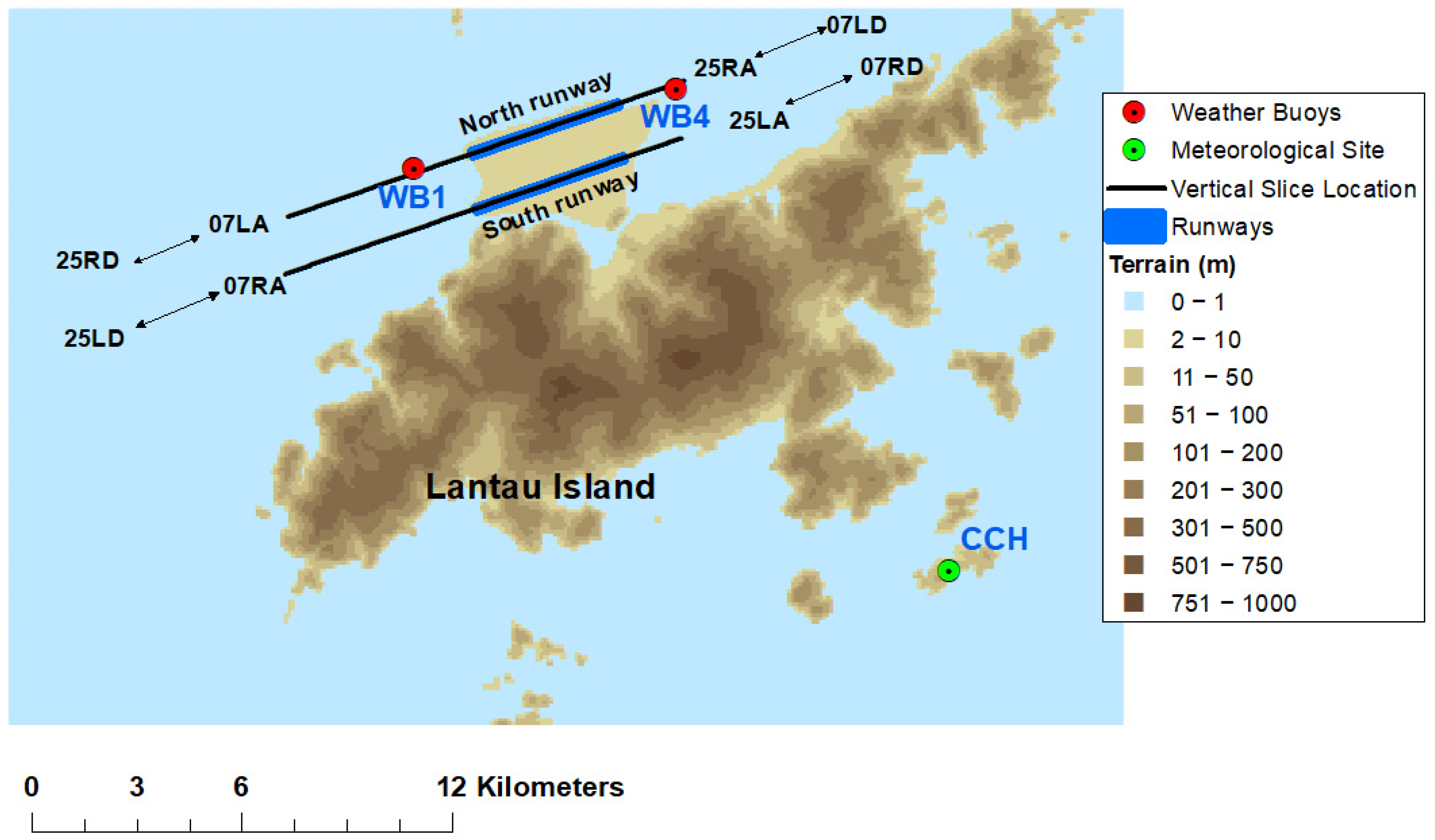
2.1. Case-Study Description

Figure 1 shows the Hong Kong International Airport study location, with the north and south runways and all runway corridors indicated. Both runways are 3.8 km in length and allow for planes arriving and departing in both directions. The runway-corridor naming convention is such that when landings and departures take place from the southwest to the northeast, the runway is named “07”, corresponding to a runway alignment of 70° as measured clockwise from the north; conversely, landings and departures from the northeast to the southwest are named “25”, corresponding to 250°. The northerly and southerly runways are categorized as either right (R) or left (L) relative to the direction of travel, and additionally as either approach (A) or departures (D). In order to model the wind shear experienced by aircraft during landing and take-off events, this study involved air-flow calculations on vertical grids of output points aligned with the runways; the ground-level signatures of these vertical grids are indicated by black lines in Figure 1. The location of the wind profiler at Cheung Chau, which provides near-real-time meteorological measurements for input into the now-casting system, is indicated (CCH), although the location of the microwave radiometer at King’s Park is beyond the extent of this map (25 km east of the airport).

The period of 4 January to 30 April 2018 was selected for this study. Note that this is the previous year in relation to that considered in [19], thus allowing for an independent test of the automatic meteorological-processing methodologies developed for that study; the same January-to-April season was considered because wind-shear events are common at HKIA in spring [8]. The pilot wind-shear reporting record for this period contains 154 wind-shear events occurring 96, 29, 15, and 12 times on runways 07LA, 07RA, 07RD, and 25LD respectively, and once on each of the 25LA and 25RA runways. Estimates for the magnitude of the headwind changes associated with wind-shear events were provided by the pilots, but the information recorded is subjective and may relate to changes in wind speed rather than headwind. The pilots recorded wind-speed/headwind changes ranging from −20 to 30 knots at heights of up to approximately 340 m. The runway location and extent, together with the information on reported heights of wind shear and typical aircraft-descent profiles, allowed for the specification of the flow-field model output domain; specifically, this was taken to be up to 6 km from the western edge of the runway in either direction. Runway corridors 07LD, 25LA, 25RA, and 25RD were excluded from the modelling and evaluation study due to the limited number of wind-shear events reported in those locations, i.e., one or zero. All reported times are local, i.e., HKT.

The meteorological-data inputs for the flow-field model were in 20 min resolution, as described in [19], whereas the pilot wind-shear reports could occur at any time. A methodology for assigning each reported wind-shear event to one or more 20 min modelling periods was developed. Specifically, where the reported wind-shear events lay between two modelling periods, both periods were classified as wind-shear events (orange time window in Figure 2). For the majority of the study, an extended time window of up to 60 min on either side of a reported wind-shear event (yellow time window in Figure 2) was considered to allow for uncertainty in terms of the input meteorological data. For instance, the wind-profiler data were recorded at Cheung Chau, which is 16 km southeast of the airport; the time taken for this air mass to pass over Lantau Island prior to arriving at HKIA could take a few hours. In addition, as discussed above, if wind shear is reported on a particular runway corridor, subsequent aircraft may be diverted from that location; consequently, the likelihood of wind shear being reported at a particular location lessens following an initial pilot report of wind shear. Results from sensitivity testing in terms of the time window associated with each pilot wind-shear report were considered (Section 3.3).

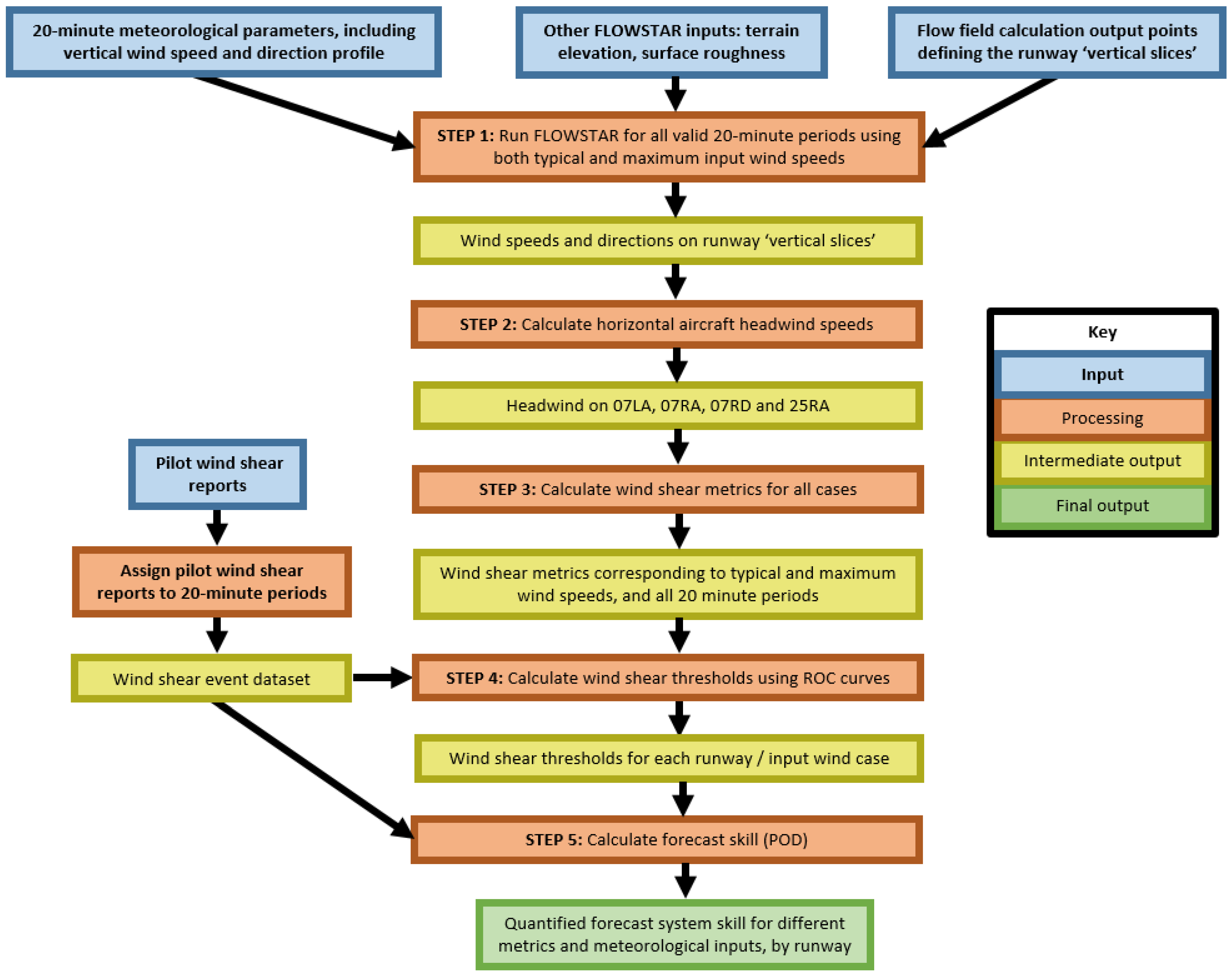
2.2. System Structure

The now-casting system structure comprises a series of data-processing tasks, labelled as steps 1 to 3 in the system flow chart (Figure 3). The evaluation process whereby the now-casting system wind-shear outputs are compared to the pilot wind-shear event dataset are described in steps 4 and 5; the methodology for generating the wind-shear event dataset required as input to steps 4 and 5 is described earlier (Section 2.1).

The meteorological-data inputs were derived from measurements available in real time using the methodology previously described [19]. A vertical grid of flow-field model output points was defined that aligns with the north and south runways, extending 6 km in either direction from the midpoint of each runway, using the approach outlined in earlier studies of wind-shear modelling using FLOWSTAR [17]. A spatial resolution of 40 m and 10 m in the horizontal and vertical directions, respectively, was prescribed, and the finer vertical resolution was required in order to capture the relatively fast variations in near-surface wind speed that occur due to the frictional drag at the earth’s surface. Python scripts handle the FLOWSTAR model runs, which were executed for each 20 min period (05, 25, and 45 min past the hour). The next steps, comprising the calculation of headwind experienced by aircraft on the different runway corridors and the subsequent derivation of a series of wind-shear metrics, were also automated using Python and R scripts.

The generation of receiver operating characteristic (ROC) curves for the multiple runway-corridor and metric combinations was calculated within a spreadsheet package. Following identification of wind-shear thresholds for each runway-corridor/wind-speed case, the skill of the now-cast was determined through calculation of the probability of detection (POD) of a wind-shear event. These skill parameters were analysed to determine which metrics are most effective at identifying wind-shear events and how sensitive the results are to input meteorological conditions, runway corridor, and model-domain extent.

2.3. Flow-Field Modelling

The FLOWSTAR model [15] has been described previously in articles relating to modelling and analysis of wind-shear events at HKIA [16,17,18]. In summary, FLOWSTAR is a quasi-linear, steady-state perturbation model that characterises the atmosphere using up to three layers, comprising a boundary layer, where, near the surface, account is taken of the impact of upwind shear and locally generated turbulence on the perturbations in mean flow; an elevated inversion layer; and a stable layer aloft. Terrain-height and surface-roughness datasets that describe the topography in the vicinity of HKIA are required for input into the model. The real-time meteorological-data inputs to the model [19] are taken to represent conditions upwind of the model domain, which extends 32 km east to west and 21 km north to south. Clearly these meteorological inputs are more representative when the wind advects directly from Cheung Chau to HKIA, which occurs approximately 15–20% of the time (considering a 30° wind sector); significantly different prevailing wind directions will most likely reduce system accuracy. The underlying FLOWSTAR system takes as input a single wind speed and direction. For this application, the input wind parameters are representative of the wind speed and direction at the top of the boundary layer. This is because earlier studies [16,18] have shown that wind shear at HKIA may be generated by mountain waves whose amplitudes are strongly dependent on the wind speed in the inversion layer.

Earlier work [17] demonstrated that multiple instances of the FLOWSTAR model can be combined to allow for the sometimes significant wind-direction changes with height. Including these variations in the modelling is important because wind shear is also generated through large-magnitude, variable changes in wind direction. An additional improvement to previous studies would be the modification of the wind-speed profile to ensure consistency with that recorded at Cheung Chau. For the current study, this was done as a post-processing step: at each height, the upwind modelled wind-speed profile was subtracted from the flow field at all calculation locations within the domain and replaced with the measured wind speed from Cheung Chau. This approach may induce small regions of reverse flow at heights where the measured wind speed is significantly smaller than the upwind modelled wind speed; however, this should happen rarely due to the upwind modelled wind-speed profile being constrained to measurements at the inversion height.

2.4. Model Inputs and Configuration

In addition to wind-speed and -direction data from the wind profiler at Cheung Chau, an atmospheric stability was estimated though the application of a marine boundary-layer algorithm, with inputs from sea-surface and air-temperature records from weather buoys in the vicinity of Chek Lap Kok. Boundary-layer height and an estimate of the temperature jump at the top of the inversion layer were derived from temperature profiles measured by the microwave radiometer at the airport.

Part of the motivation for the meteorological pre-processing methodology [19] was to develop techniques for filtering the modelled time periods by excluding cases that were unlikely to generate mountain waves—for instance, low wind speed and no temperature jump at the top of the boundary layer, with the latter condition making the atmospheric conditions unable to generate resonating trapped waves. However, the current study highlighted that a large number of wind-shear cases are related to synoptic wind conditions—for instance, sharp wind-direction changes with height, rather than localised wind shear generated by terrain elevation. For this reason, the meteorological filtering was removed and over 85% of the time periods were modelled. The remaining cases could not be modelled due to insufficient and/or poor-quality meteorological input data. For instance, the wind profiler has a data quality-control flag that indicates whether the measurements are valid, estimated, suspect, or invalid; only valid and estimated data are used as inputs to the system.

For this model application, the primary wind-parameter input to FLOWSTAR was the speed in the inversion layer. Earlier work [16] demonstrated the sensitivity of modelled mountain waves to the magnitude of this parameter, which resulted in subsequent studies considering a range of wind speeds as input. Specifically, typical (average) and maximum inversion-layer wind speeds were both modelled. As wind-profiler measurements were taken at relatively large vertical spacing in comparison to the inversion-layer depth, the typical and maximum values were the same in a number of cases.

2.5. Derivation of Wind-Shear Metrics from Flow-Field Modelling Outputs

Previous studies have investigated metrics suitable for quantifying wind shear. For instance, in a study on the use of LIDAR for wind-shear reporting at HKIA [6], a wind-shear severity factor was defined as:

$$S=\frac{\Delta V^3}{H V_{\mathrm{app}}}$$

(*)

where $\Delta V$ is the total change of wind along the glide path, $H$ is the ramp length, and $V_{\mathrm{app}}$ is the normal approach speed of the aircraft. The wind-shear ramp length is the distance over which there is a sustained change in headwind corresponding to the wind-shear event. The earliest FLOWSTAR studies modelling wind shear along an aircraft trajectory [16,18] demonstrated that the model was able to predict the sharp changes in headwind that cause adverse wind shear. A subsequent study [17] derived observed and modelled headwind gradients along the flight path in an attempt to distinguish between favourable and unfavourable landing conditions; these headwind gradients broadly correspond to $\Delta V/H$ using the notation from (*). This work highlighted that sharp headwind gradients may relate to flow structures that can be identified by consideration of 2D vertical headwind slices (Figure 4). The current study involved automating the calculations of not only horizontal headwind gradients but also corresponding vertical gradients; an indication of how horizontal and vertical gradients are calculated is given in Figure 4 adjacent to a modelled complex-flow structure.

As discussed earlier, considerable changes in headwind are more problematic to pilots in strong headwind conditions. For this reason, metrics corresponding to the product of the headwind and the headwind gradient were derived and assessed in terms of their ability to quantify wind shear; these parameters correspond to $\Delta V^2/H$ in the notation introduced in Equation (*) and hereafter are referred to as either horizontal or vertical accelerations. Although the majority of reported adverse landing/take-off conditions are associated with positive wind shear (i.e., where headwind increases), a small proportion is associated with negative wind shear (i.e., where headwind decreases), so both positive and negative accelerations were calculated.

Developing tools to automate the derivation of wind gradients from modelled headwinds facilitates the calculation of a range of metrics. For instance, with reference to [7], where the wind-shear severity factor is proportional to $\Delta V^3$, the magnitude of the headwind at the location of maximum acceleration can be considered. In addition, the relative importance of considering the sign of the acceleration or headwind can be investigated.

Table 2. Metric summary, including mathematical notation, and summary of justification for inclusion in the study; all metrics are calculated in both horizontal and vertical in relation to the 2D vertical slices aligned with the runways.

Metric Desciption	Mathematical Notation $(\mathbf{Headwind}{\mathit{U}}_{\mathit{H}}$$\mathbf{Headwind}\mathbf{Gradient}\mathit{d}{\mathit{U}}_{\mathit{H}}/\mathit{d}\mathit{s})$	Justification
Max. value of acceleration	$\mathrm{Max}\left[U_H\frac{d{U}_H}{ds}\right]$	The product of the headwind and headwind gradient amplifies the impact of sharp changes in headwind.
Min. value of acceleration	$\mathrm{Min}\left[U_H\frac{d{U}_H}{ds}\right]$
Max. magnitude of both acceleration metrics	$\mathrm{Max}\left(\left|\mathrm{Max}\left[U_H\frac{d{U}_H}{ds}\right]\right|, \left|\mathrm{Min}\left[U_H\frac{d{U}_H}{ds}\right]\right|\right)$	Test sensitivity with regard to minimum and maximum values
Headwind at the max. value of acceleration	$\left|{U_H|}_{\mathrm{Max}\mathrm{acceln}}\right|$	Following previous work where the severity factor was proportional to the cube of the headwind
Headwind at the min. value of acceleration	$\left|{U_H|}_{\mathrm{Min}\mathrm{acceln}}\right|$
Max. magnitude of both headwind metrics	$\mathrm{Max}\left(\left|{U_H|}_{\mathrm{Max}\mathrm{acceln}}\right|, \left|{U_H|}_{\mathrm{Min}\mathrm{acceln}}\right|\right)$	Test sensitivity with regard to minimum and maximum values

summarises six metrics that were considered in this study. The mathematical notation used to describe the metrics refers to the headwind,$U_H$, and the distance over which the gradient is calculated, $ds$, where $ds$ is directed along the runway for the horizontal metrics and upwards for the vertical metrics.

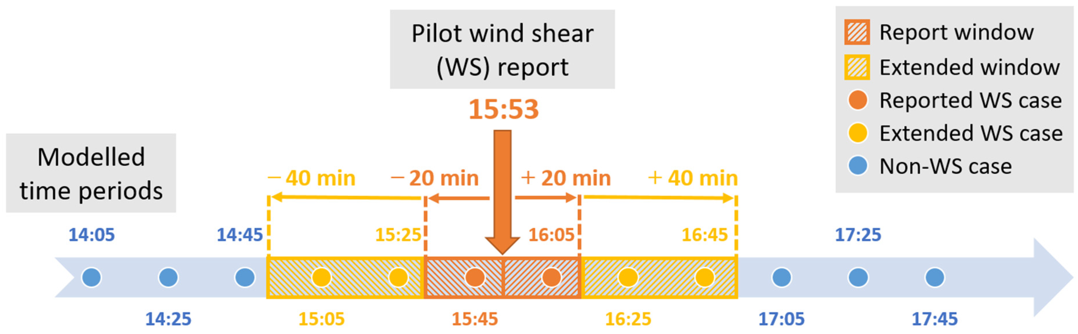
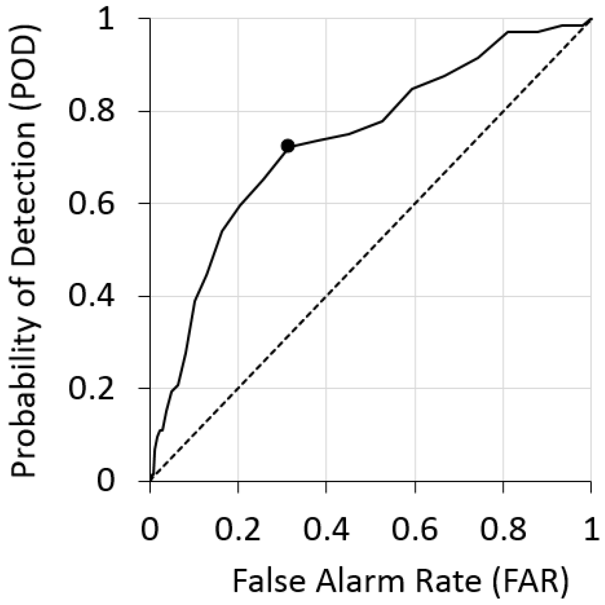
2.6. Now-Cast Skill Analysis

Now-cast skill is commonly described in terms of four parameters, a, b, c, and d, which quantify the number of observed and modelled events (

Table 3. Definition of event parameters.

		Event Observed
		Yes	No
Event Modelled	Yes	a	b
	No	c	d

). The likelihood of the now-casting system predicting a particular event is defined as the probability of detection (POD): $a/\left(a+c\right)$, and the likelihood of incorrectly now-casting an event is the false-alarm rate (FAR): $b/\left(a+b\right)$. For a system in which all events are recorded accurately, a reliable now-cast is one that has a high POD close to unity and a low FAR close to zero. For the current study, however, where it was noted that there were likely to be many unobserved wind-shear events, FAR was likely to be high; as such, the focus of this study was on relative magnitudes of the POD parameter.

Receiver (or relative) operating characteristic (ROC) curves can provide an indication of the sensitivity of a particular metric’s ability to now-cast events. ROC curves are generated through a sequence of calculations: firstly, the metric is calculated for each modelled period, which allows for the definition of multiple metric-category bins (around 50) that encompass the range of metric values. Then, the frequency of wind-shear and null wind-shear events are derived for each metric bin, leading to the calculation of POD and FAR values for each metric category; an ROC curve is then generated by plotting POD against FAR.

An ROC curve quantifies how the number of correctly modelled events relates to the magnitude of the threshold that can be used to detect events. An example is shown in Figure 5, with the POD and FAR values shown on the vertical and horizontal axes, respectively. The graph starts at (0,0) because if the threshold is set to zero, no events are detected correctly (POD = 0), but no events are incorrectly detected, either (FAR = 0). The graph ends when all events have been detected (POD = 1, FAR ≤ 1). Now-casts with better skill have ROC curves with vertical gradients that are much greater than unity, with the point farthest from the FAR = POD line indicating parameters that maximise POD for low values of FAR, ensuring that POD must be greater than FAR (black dot in Figure 5); these parameters can be identified through calculation of the product of POD $\times$ (1 − FAR) $\times$ (POD − FAR), with the last term in this expression ensuring that this metric identifies the maximum positive distance between the 1:1 line and the ROC curve. For this study, parameters identified using this methodology were used to define thresholds for assessing now-cast accuracy in terms of POD for all metrics and runways.

3. Results

The results presented in this section relate to the period from January to April 2018. Section 3.1 presents the outcomes of the analyses of the pilot wind-shear reports for this period. A summary of the meteorological data used as input to the system is given in Section 3.2. The flow-field and wind-shear metric calculations are described in Section 3.3 and the now-casting skill results are presented in Section 3.4. The results of some sensitivity testing of the model parameters are given in Section 3.5.

3.1. Pilot Wind-Shear Report Summary

Table 4. Summary of the subset of modelled cases corresponding to pilot wind-shear reports; * the number of cases differs for typical and maximum’ inversion-layer wind-speed cases due to the typical cases requiring more comprehensive meteorological-data input parameters than the ‘maximum cases; runway corridors 07LD, 25LA, 25RA, and 25RD were excluded from the modelling due to insufficient corresponding pilot wind-shear reports.

	Count of Modelled Wind-Shear Cases (Total Number of Reports)			Along-Runway Modelling Extent from Southwest to Northeast
	Approaches		Departures
Runway	North	South	South	−6000 to 0	0 to 6000	−6000 to 6000
07LA	88 t/96 m * (96)			✓	✗	✓
07RA		27 (29)		✓	✗	✓
07RD			15 (15)	✗	✓	✓
25RA	12 (12)			✗	✓	✓

summarises the number of modelled wind-shear cases and the total number of reported wind-shear events by runway corridor (first column). The number of wind-shear events included in the model dataset is not always equal the number of pilot reports. This is partly due to multiple wind-shear reports occurring during the same 20 min time interval, and also because a subset of cases was not modelled due to unavailability of good-quality wind-profiler measurements, which restricts the calculation of the average wind speed in the inversion layer. The events were categorised into approaches or departures and runway (columns two to four).

The table shows that the majority of wind-shear events were reported for aircraft landing on the northerly runway. Of note, therefore, is that the initial studies of wind shear at HKIA using FLOWSTAR [16,18] focussed on a single hazardous wind event that occurred on the southerly runway, although wind-shear events on both runways were considered in a more recent study [17].

The full horizontal extent of the modelled vertical slice associated with each runway was 12 km (Figure 4). In earlier work, the full 12 km domain was modelled, but for this study, the sensitivity of the results to the along-runway extent was investigated because, for instance, an aircraft arriving from a southwesterly direction would only be exposed to flow structures to the southwest of the airport; columns five to seven indicate the horizontal extents that were considered.

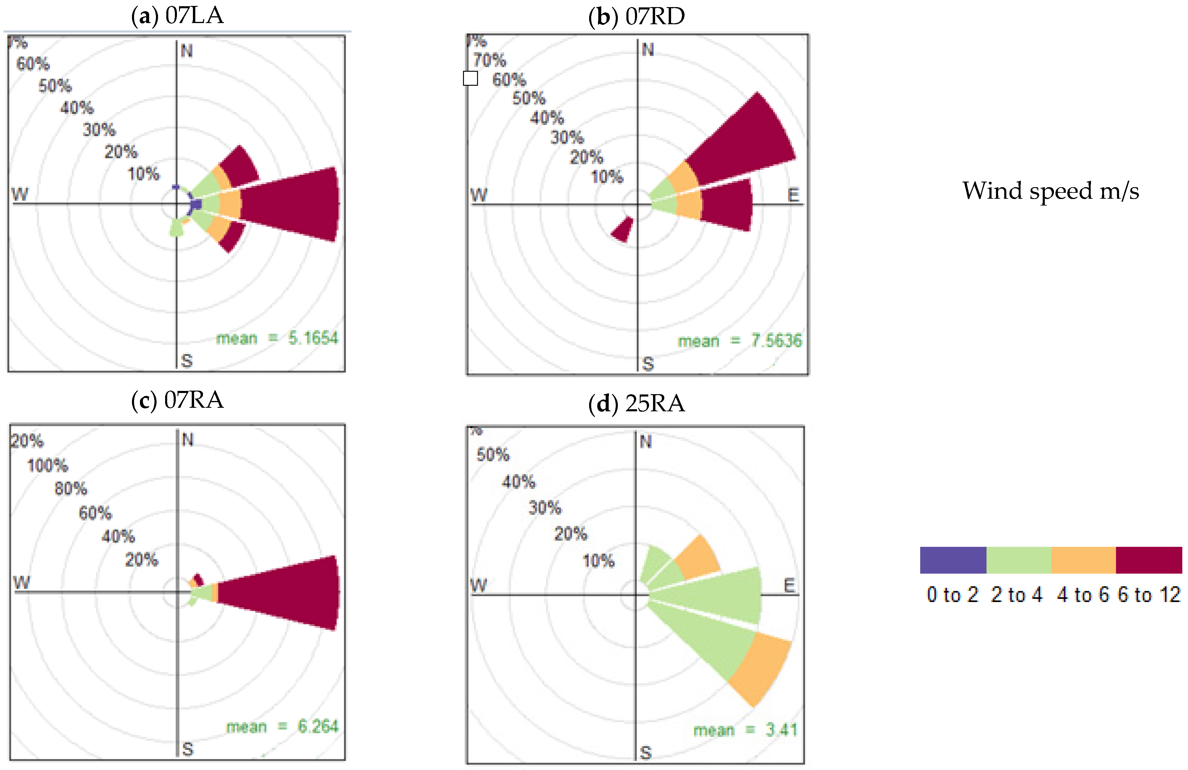
3.2. Meteorological-Data Summary

The meteorological-data input requirements for FLOWSTAR are discussed in earlier work, with Table 2 of [17] summarising the required parameters for that study, in which a small number of meteorological cases was analysed.

Table 5. Data summary of meteorological parameters required as input for FLOWSTAR for the period from January to April 2018.

Parameter		Units	Minimum	Average	Maximum
Wind	Maximum speed in the inversion layer	m/s	0.2	7.1	25.1
	Typical speed in the inversion layer	m/s	0.0	4.0	20.6
	Direction at max speed	degrees	0	82	360
	Direction at typical speed	degrees	0	111	360
Surface-sensible heat flux		W/m2	−44	7	140
Boundary-layer height		m	200	211	550
Inversion-layer temperature jump		K	0.0	2.9	17.8
Buoyancy frequency (above the inversion layer)		1/s	0.005	0.015	0.020

summarises the range of values associated with the same set of required parameters for the four-month period considered in the current work.

Wind speeds in the inversion layer had maximum values of 21 m/s for the typical wind-speed case and 25 m/s for the maximum wind-speed case. The average wind directions were similar for both wind-speed cases, close to easterly; this wind direction corresponded to the flow advecting over the slightly less elevated parts of Lantau Island at the eastern end. A range of atmospheric stabilities was modelled, from stable through convective. The modelled boundary-layer heights were relatively low, with the maximum height being only 550 m. This may be a consequence of the methodology used to estimate the boundary-layer height from temperature-profile data; microwave-radiometer estimates of temperature decrease in accuracy with height beyond a few hundred metres and cannot resolve the sharp potential temperature changes associated with the location of the top of higher boundary layers. This uncertainty in boundary-layer height estimates was unlikely to significantly influence the outcomes of the current study, wherein adverse conditions were more likely to be associated with low boundary-layer heights. Temperature-jump magnitude is an important parameter when studying the formation of mountain waves, with higher values more likely to lead to large-amplitude waves, with values ranging up to 18 K. Limits were applied to constrain the buoyancy-frequency values above the inversion layer, which were difficult to estimate from the microwave-radiometer temperature profiles; specifically, minimum/maximum values of 0.005/0.020 s⁻¹ were applied.

3.3. Flow-Field and Wind-Shear Metric Calculations

Flow-field calculations were performed for all 20 min periods from January to April 2018 for which a full set of input meteorological parameters (Table 5) was available. Headwind values corresponding to each runway corridor were derived from the 3D wind-field values; the six wind-shear metrics (Table 2) were then calculated. Although run times for a single 20 min period were short (approximately 5 min), the large number of periods considered (5913 for typical and 6656 for maximum wind-speed conditions) and the multiple configurations to model (four runway corridors and two wind-speed conditions) made the total run time for this study significant. The processing time for the derivation of headwind from the 3D flow field was a few minutes, but the complete set of metric calculations for the full four-month period took a number of hours.

At this stage of the study, all six wind-shear metrics were calculated. Figure 6 provides a graphical explanation of the methodology used to derive the metrics in relation to a modelled headwind slice, with corresponding synoptic winds presented in Figure 7. A second example is shown in Figure 8, with the corresponding synoptic winds presented in Figure 9. These examples were selected in order to demonstrate the differing causes of wind shear at the airport: trapped waves (Figure 6) and strong directional wind shear (Figure 8).

All metrics were calculated as minimum or maximum values for each horizontal location, measured as the distance from the westerly edge of the model domain. The upper plot, Figure 6a, shows the minimum and maximum vertical-acceleration parameters in relation to the vertical headwind slice (Figure 6b). The maximum vertical acceleration remained approximately constant and, as the wind speed decreased approximately monotonically with the height above the ground, the minimum vertical accelerations remained close to zero for the majority of the domain presented. Horizontal acceleration values (Figure 6c) were much smaller in magnitude than the corresponding vertical parameters because they were not influenced by the underlying vertical wind-speed profile. The maximum horizontal acceleration corresponds to increases in headwind from left to right in Figure 6b, and the minimum horizontal acceleration corresponds to decreases. Where there were large, wave-like structures, the horizontal acceleration parameters oscillated, peaking in magnitude where the gradients were strong and headwinds relatively high. The wind barbs on Figure 6b show the measured wind-speed and -direction profile recorded upwind of the model domain. This case had little change in wind direction with height, remaining in the 70°-to-80° wind sector and with a relatively high wind speed at the top of the modelled domain (12 m/s at 400 m). Figure 7 shows the modelled synoptic wind vectors at a height of 100 m. The primary plot shows the large wind magnitude and directional changes over the model domain. Although some of the high winds occurred just downwind of the highest terrain, there were also strong winds over the sea, which relate to mountain waves propagating downstream of the peaks. The inset adjacent to the airport shows the approximate area to which Figure 6b corresponds, allowing for a visualisation of the horizontal flow that generated the headwind variations.

Thus, the combination of wind speed and direction shown in Figure 6 resulted in moderately large acceleration parameters combined with high headwinds. The modelled oscillating headwind values suggests that trapped waves were being generated; an inspection of the corresponding FLOWSTAR input parameters supported this hypothesis, with near-neutral atmospheric conditions (a surface-sensible heat-flux value of −0.3 W/m²) combined with a large temperature jump at the top of the boundary layer (10.5 K).

Figure 8 presents the same series of plots for a very different headwind pattern. Here, the flow structure was dominated by the vertical wind shear generated by the upwind profile (refer to the wind barbs on Figure 8b). Wind magnitudes were smaller than in the previous case and the wind directions ranged from 160° to 345° below 150 m, leading to tailwinds. Figure 9a,b shows synoptic winds corresponding to 100 m and 200 m above ground, respectively, and a strong directional shear as well as a decrease in wind speed with height was demonstrated (shown in the wind barbs on Figure 8b). Also of note in these plots is that high wind magnitudes corresponded closely to terrain elevation, without the additional off-shore flow structures seen in the trapped-wave case. In terms of the wind-shear metrics, the vertical-acceleration parameters presented in Figure 8a showed symmetry between the minimum and maximum values, and magnitudes of both parameters were greater than in Figure 7. Conversely, the horizontal-acceleration metrics were considerably smaller in magnitude than the corresponding trapped-wave case because headwind values varied little with distance along the runway (Figure 8c).

The modelled headwinds presented in Figure 8 led to large-magnitude vertical-acceleration parameters combined with moderate wind speeds. The synoptic meteorological conditions differed considerably from the trapped-wave cases, with a surface-sensible heat-flux value of 45 W/m², i.e., convective conditions.

Figure 6 and Figure 8a,c present examples of how the minimum and maximum horizontal- and vertical-acceleration parameters varied with horizontal distance along the vertical slices. The acceleration-metric quantities (Table 2) were the maximum or minimum of these values, and a further metric considered was the maximum absolute value of either of these metrics. An additional set of metrics was taken as the magnitudes of the headwind values at the locations of the acceleration metric quantities and, finally, the maximum absolute value of these parameters.

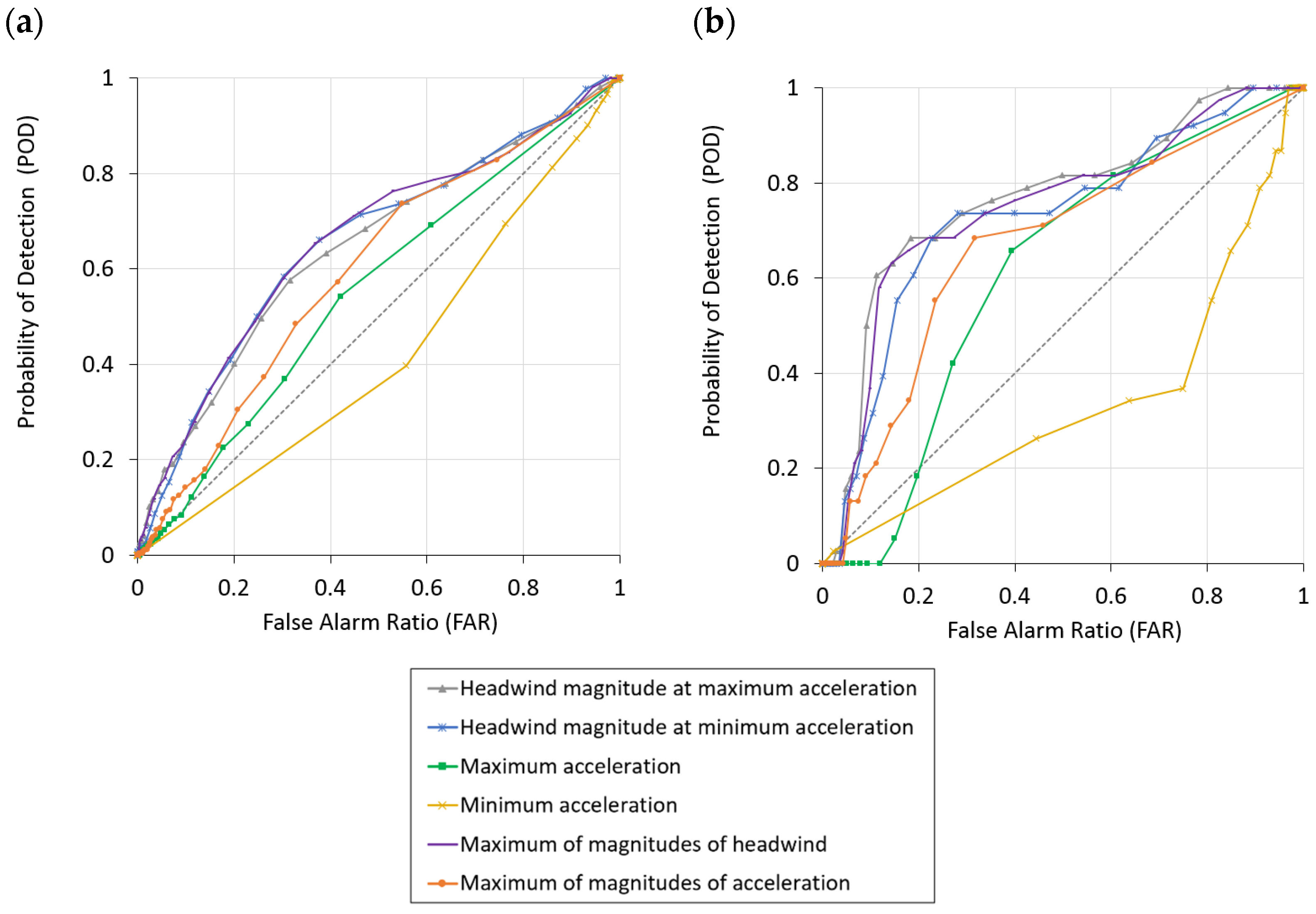
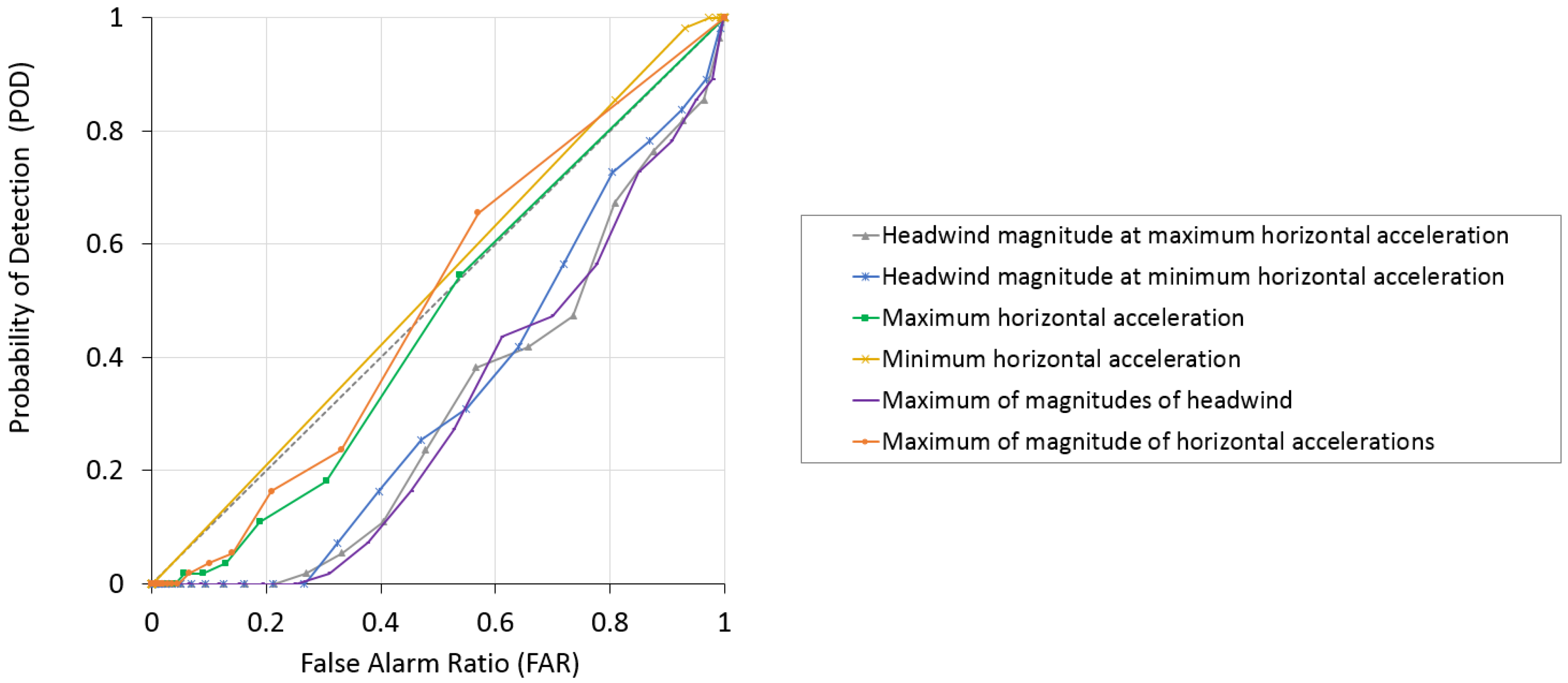
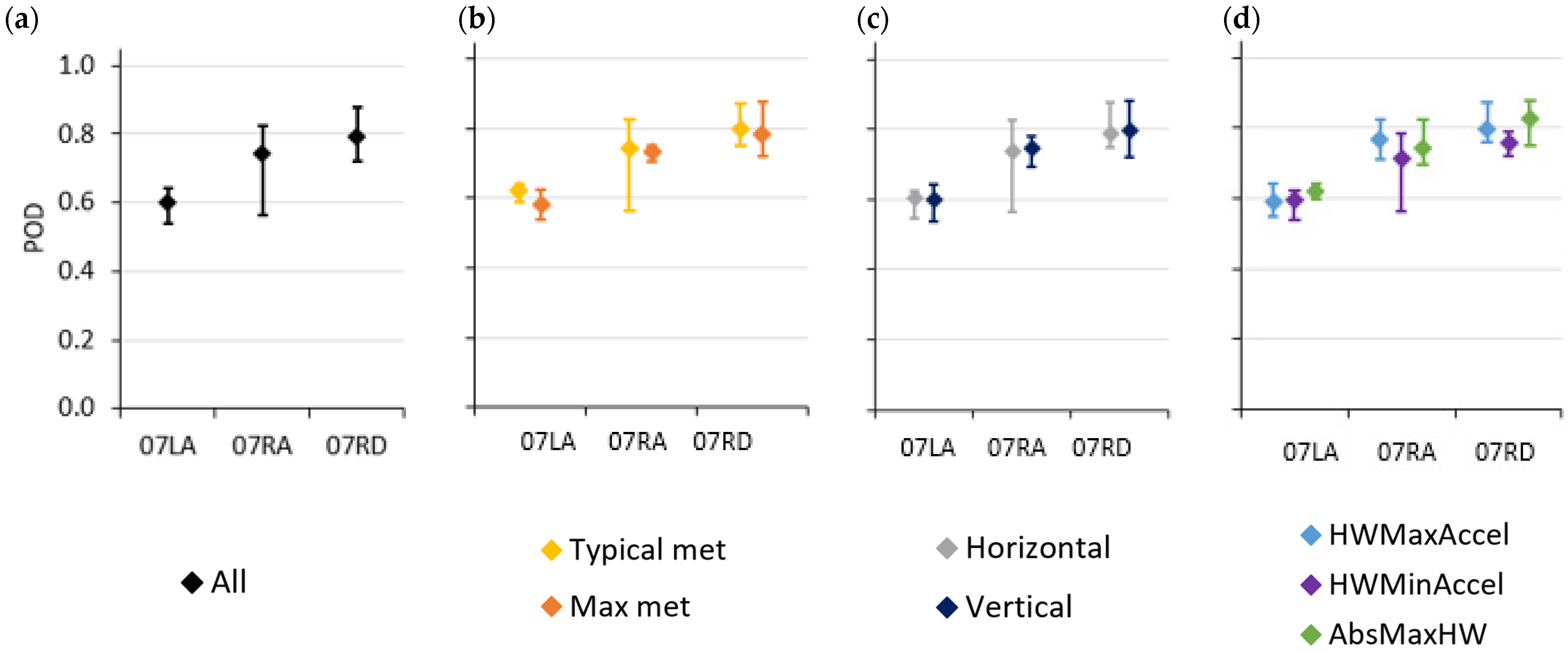
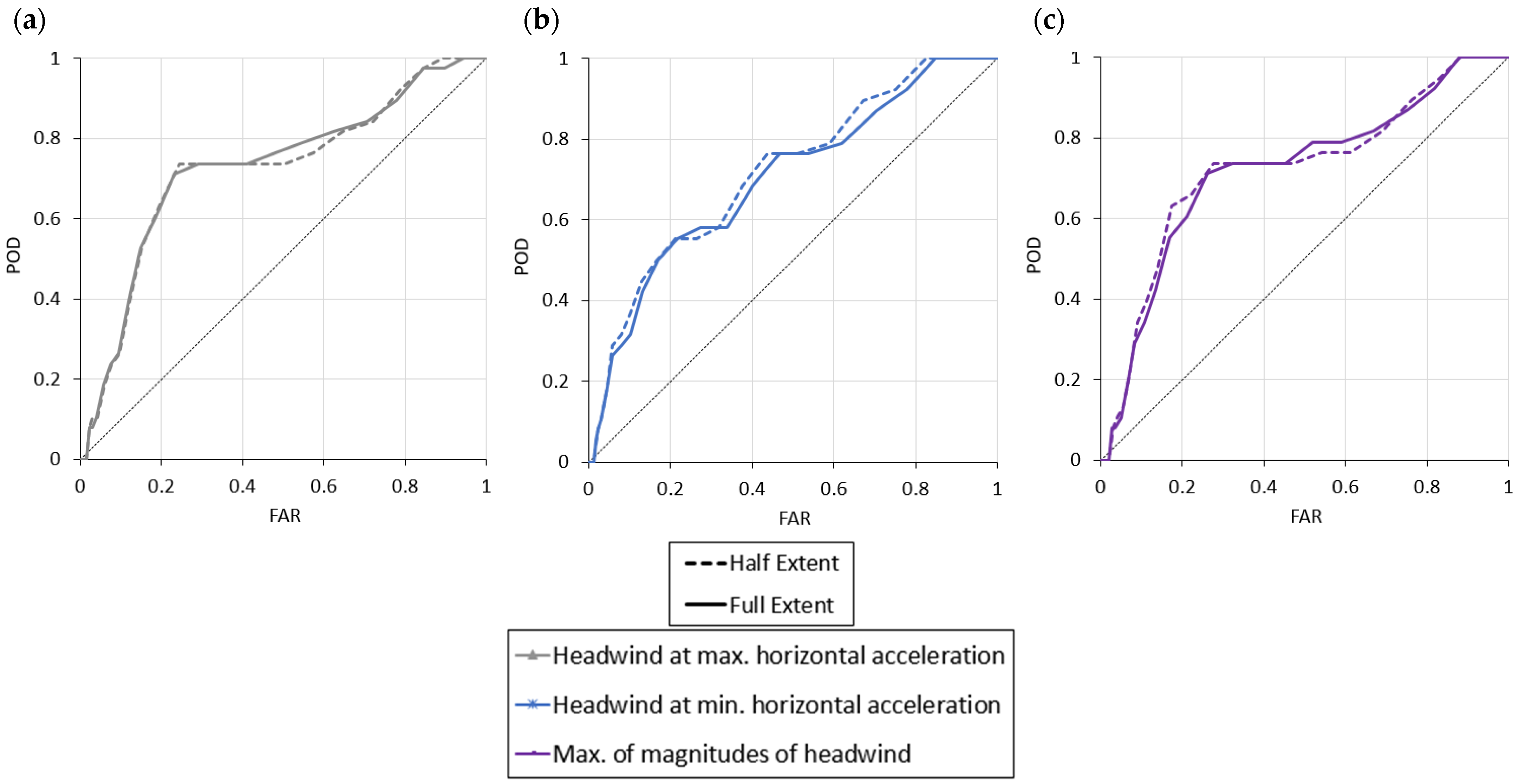
3.4. Now-Casting Skill Analyses

Acceleration and headwind metrics (Table 2) were calculated and used to generate ROC curves and hence the relative skill of each type of metric assessed. Figure 10 presents two example sets of ROC curves; Figure 10a presents a maximum wind speed in a horizontal-acceleration case, and Figure 10b presents the results for a typical wind speed in a vertical-acceleration case. Here, as for the majority of the ROC curves generated, the skill of the headwind metrics that relate to the location of the maximum and minimum values of the acceleration were better than the skill of the underlying acceleration parameter. Only the headwind metrics were evaluated in subsequent analyses due to their better performance. The inter-comparison of Figure 10a,b also suggests that the vertical-acceleration parameters performed better that the horizontal parameters, but this is not true when comparing results from the same runway corridors.

The calculations for the 25 runway corridors were fundamentally the same as for the 07 runway corridors, apart from the headwind calculation, which was rotated by 180 degrees, i.e., the aircraft was travelling from a northeasterly direction rather than southwesterly. Figure 11 presents the series of ROC curves for 25RA. These curves indicate that the metrics used to identify wind shear for the 07 runway corridors had no skill in terms of identifying wind shear for the 25RA runway. Analysis of the meteorological conditions associated with the pilot wind-shear reports discussed below helps to explain this.

Figure 12 presents the wind roses associated with all wind-shear cases for the four runway corridors studied (Table 4). Here, the wind data presented correspond to values recorded by the Cheung Chau wind profiler at the time and elevation of the pilot-reported wind shear. The wind direction ranges for the 25RA runway corridor were similar to those for the 07 runway corridors, indicating that the conditions were less than ideal because landings occurred with the wind advecting in the same direction as the aircraft. Wind-speed magnitudes corresponding to the 25RA pilot reports (mean wind speed of 3.4 m/s) were significantly lower than for the other runway corridors (mean wind speeds in the range 5.2 m/s to 7.6 m/s); this difference in wind magnitude explains why the high-headwind thresholds were not appropriate for the 25 runway corridor. The wind-shear cases for the easterly approaches could have been caused by local fluctuations in southerly winds, and, noting that all reported 25RA wind-shear cases occurred between 03:20 and 09:20, a possible explanation is the influence of land breezes.

Following the methodology described in Section 2.6, ROC curves were used to identify the most suitable threshold criteria.

Table 6. Resultant wind-speed (m/s) thresholds calculated from the ROC-curve analysis. A quantitative indicator of performance is given in brackets for each scenario (with better performance indicated in bold, corresponding to POD × (1 − FAR) × (POD − FAR) > 0.2).

		Vertical		Horizontal
Metric	Runway	Typical	Max	Typical	Max
Magnitude of headwind at maximum acceleration	07LA	6.0 (0.16)	6.5 (0.12)	6.0 (0.17)	5.5 (0.10)
	07RA	7.5 (0.28)	8.5 (0.25)	7.0 (0.28)	6.5 (0.19)
	07RD	6.5 (0.28)	6.0 (0.21)	5.0 (0.22)	5.0 (0.18)
Magnitude of headwind at minimum acceleration	07LA	6.0 (0.17)	6.0 (0.10)	6.0 (0.15)	5.0 (0.12)
	07RA	7.0 (0.24)	7.0 (0.17)	7.0 (0.15)	5.0 (0.11)
	07RD	5.5 (0.24)	6.0 (0.20)	6.5 (0.27)	6.0 (0.23)
Maximum magnitude of both headwind metrics	07LA	6.5 (0.19)	6.5 (0.13)	6.5 (0.17)	5.5 (0.12)
	07RA	8.5 (0.26)	8.5 (0.24)	7.0 (0.25)	7.5 (0.20)
	07RD	6.5 (0.26)	6.0 (0.23)	6.5 (0.27)	6.0 (0.23)

presents the thresholds separately for each of the three headwind metrics corresponding to both the vertical and horizontal accelerations and the two wind-speed cases for the three 07 runway corridors; the quantitative parameter used to quantify the threshold is also given. These results are the first that indicate the trends in skill of the now-casting system; specifically, performance is best for the 07R runway corridors and the combined metric.

Applying these thresholds allowed for the calculation of POD values; these are summarised in Figure 13. As indicated by the threshold quantification above, the performance was best for runway corridor 07RD (Figure 13a). The typical wind-speed modelling appeared to perform slightly better in comparison to a maximum wind-speed approach (Figure 13b); most likely this relates to the issue of having had relatively few measurements within the inversion layer previously mentioned, which added to uncertainty in terms of a specification of a single maximum wind-speed value. There was a slight indication that headwinds associated with the vertical-acceleration parameter were a better metric than the corresponding horizontal parameter (Figure 13c). Since the vertical-headwind parameter could be used to identify wind shear resulting from both trapped waves and directional wind shear (Figure 6a and Figure 8a) but the horizontal wind-shear metric was most relevant to the flow structures resulting from localised oscillating flow (Figure 6c), this result suggests that both types of wind shear were present in this dataset. The final graph in this series (Figure 13d) indicates that the headwind associated with the minimum acceleration performed less well in comparison to the other two headwind metrics. Overall, the POD values presented in Figure 13 behaved consistently across runways, which boosts confidence in the conclusions presented above.

3.5. Further Sensitivity Testing

Using a computationally inexpensive model (as opposed to, for instance, a mesoscale meteorological model) facilitates the testing of different model inputs. This was demonstrated through the use of different input meteorological conditions i.e., typical and maximum wind speeds; furthermore, six metrics quantifying horizontal and vertical wind shear were calculated. This section presents results of some additional sensitivity testing that was undertaken during the study.

Table 4 summarises the along-runway extents that were considered for each runway corridor. Figure 14 presents the results of the sensitivity of ROC curves to this horizontal extent for the three headwind metrics for one example runway corridor (07RA) and one set of input meteorological conditions (typical). The graphical results presented in this figure did not show a clear trend in terms of better performance for either the half or full runway, but when the corresponding performance indicators were collated (

Table 7. Sensitivity of the quantitative indicator of performance (better performance indicated in bold with +1 indicative of ideal performance) to the horizontal extent of data included in ROC calculations. The full runway length or the half-runway extent is based on direction of approach. 07RA runway corridor, typical met, horizontal acceleration, 40 min wind-shear time window.

	Metric Performance
Runway Extent	Headwind at Max. Acceleration	Headwind at Min. Acceleration	Max. of Magnitudes of Headwind
Half	0.275	0.148	0.246
Full	0.260	0.145	0.236

), the half runway results were slightly better, although differences between the configurations were not statistically significant. The half runway performed better for all runways, which is reassuring in terms of the study configuration because restricting the modelled domain to a half runway is a better representation of the real-world spatial extent, i.e., when landing, aircraft have usually touched down before the midpoint of the runway, and aircraft use at least half the runway for ground roll to gain sufficient speed prior to lift off. The now-casting skill analyses presented in Section 3.4 correspond to the half-runway model configuration.

Sensitivity to the time window (Figure 2) used in the calculations was determined in the preliminary stages of the project. At that stage, performance was better for the 40 min time window, so this value was used in subsequent calculations; further system refinements were carried out during the study, but a time-window sensitivity analysis was not repeated until the final stages.

Table 8. Sensitivity of the quantitative indicator of performance (better performance indicated in bold with +1 indicative of ideal performance) to the extended wind-shear time window. 07RA runway corridor, typical met, horizontal acceleration, half runway extent.

	Metric Performance
Extended Time Window (mins)	Headwind at Max. Acceleration	Headwind at Min. Acceleration	Max. of Magnitudes of Headwind
20	0.343	0.170	0.309
40	0.275	0.148	0.246
60	0.214	0.120	0.206
80	0.188	0.113	0.194

summarises the sensitivity of the quantitative performance indicator (i.e., POD × (1 − FAR) × (POD − FAR)) to the time window for the 07RA runway corridor and typical meteorological conditions. These results indicate that a 20 min time window led to better performance compared to the longer time windows because for all performance metrics, the quantitative indicator of performance increased toward unity with a decrease in the time window. As is the case for the sensitivity testing relating to the runway extent, this result, whereby performance was better when a more precise time period was considered, indicates that the system performed consistently with regard to the input meteorological-measurement datasets.

4. Discussion

This paper describes a wind-shear now-casting system for Hong Kong International Airport and presents evaluation results corresponding to the application of the system for the historical four-month period from January to April 2018. The work is a continuation of previous studies [16,17,18] in which the core flow-field modelling component of the system was configured to replicate the generation of mountain waves that are generated downwind of Lantau Island that impact aircraft movements at the airport. The data processing of real-time meteorological measurements into a format that can be used by the system is a non-trivial exercise due to the requirement for the derivation of inversion-layer parameters, and has been described elsewhere [19].

The method for the assignment of wind-shear events to modelled time periods was outlined, followed by a description of the system structure. A brief overview of the flow-field modelling component of the system was provided, including details of the required system inputs. Motivation for the six wind-shear metrics selected was given, and the approach taken to quantifying now-cast skill in terms of the probability-of-detection (POD) parameter was described.

The study results commenced with a quantification of the pilot wind-shear reports: 152 reports, with the majority relating to the 07LA runway corridor. Of relevance to the calculation of the now-cast skill parameters is that there is most likely a number of wind shear events that occur during the modelled period that were not reported. This is because flights do not occur at all times during the day and night; in addition, when pilots report wind shear, evasive action may be taken—for instance the flight may be diverted to another runway or airport. Consequently, the now-casting system false-alarm rate is high because in a number of cases the system predicts wind shear but there is no corresponding record. The meteorological conditions during this four-month time period were predominantly neutral and convective due to the combination of relatively high wind speeds and the marine heat-flux environment, with the prevailing inversion-layer wind direction being easterly with a mean wind speed of 7 m/s. The consideration of 20 min periods, two wind conditions (typical and maximum wind speed in the inversion layer), and two runways (south and north) led to the generation of a large dataset of headwind conditions for analysis: over 27,000 cases. The metric calculations were described using two example cases corresponding to a trapped-waves case and a large directional wind-shear case. Example ROC curves were presented from the total of 192 generated. An expression was defined that quantifies ROC-curve behaviour, which was used to identify which wind-shear metrics demonstrate the best performance. The three metrics derived from the magnitude of the headwind at the locations of maximum and minimum accelerations had more skill compared to the acceleration metrics. This is because changes in wind shear are less disruptive when headwind magnitudes are low, i.e., wind conditions are adverse when sharp changes in headwind occur during high-headwind episodes. The aggregate metric, defined as the maximum magnitude of headwind at locations of both the minimum and maximum accelerations, performed best. In addition, system skill was better for the southerly runway compared to the northerly runway. POD values for the westerly aircraft movements were in the range of 0.6 to 0.8, indicating that the system demonstrated some skill in terms of identification of wind shear. The relatively poor performance of the selected metrics in predicting wind shear for the easterly 25RA runway corridor relates to wind-shear cases with low-magnitude tailwinds, possibly due to the interaction of land breezes with prevailing southerly winds. The sensitivity of the results to system inputs and configuration was presented, specifically comparing performance when modelling using half-runway and full-runway output domains, as well as time windows ranging from 20 min to 80 min. These spatial and temporal evaluations had broadly consistent conclusions, i.e., restricting the modelling to better represent the exact real-world situation led to better performance; however, spatial and temporal incompatibilities associated with model inputs means that it was not possible to be overly precise in terms of where and when wind-shear events occur.

This system could be developed to run operationally on a high-specification, multi-core PC. Real-time meteorological inputs (microwave radiometer, wind profiler, Cheung Chau surface anemometer, and weather-buoy data) would be transferred via bespoke application-programming interfaces (APIs) to the PC. A Windows task scheduler could be used to run the required meteorological pre-processing scripts [19] prior to executing the FLOWSTAR model runs. The three headwind metrics relating to the magnitude of the headwind at the locations of the minimum and maximum accelerations would then be derived from the FLOWSTAR outputs for each runway corridor using both input meteorological datasets. Metric values would be compared to the proposed threshold values (Table 6) in order to determine whether the wind conditions are adverse, giving rise to an alert.

There is a number of items that could be refined within the system. The wind-shear modelling time corresponds to the microwave-radiometer measurement time, and the data were extracted from the wind-profiler dataset for the same time. In reality, for easterly winds, the time taken for the air mass to pass from Cheung Chau to HKIA, a distance of approximately 16 km, ranges from less than an hour to up to a few hours, depending on wind speed; this time lag was considered in an earlier study [18] but was not allowed for in the current system. Wind-speed and -direction information recorded at the airport in real time could be used to refine headwind estimates at the airport; for instance, the Doppler LIDAR [6] data could be used as an input to the system. With regard to the acceleration metrics, the use of the product of the magnitude of the headwind and the magnitude headwind gradient may demonstrate slightly better performance than the current metrics, where the signs of headwind and the headwind gradient are included in the calculations. Finally, the sensitivity testing suggests that using a 20 min time window to link wind-shear alerts to modelled time periods would be better than the 40 min window condition used in this study. Operationally, it would be advisable to execute multiple system configurations simultaneously—for instance, taking current and historic wind-profiler data from Cheung Chau, as well as differing estimates of wind speed in the inversion layer. Such an approach would lead to an ensemble-model result that, together with data from other modelling systems and instrumentation, may produce a relatively accurate indication of wind shear. It is recommended that all these refinements be undertaken prior to the development of an operational now-casting system.

A consequence of the time taken for the air mass to pass from Cheung Chau to HKIA is that, for the subset of easterly prevailing wind directions, the system could be considered a short-term forecast, although other inputs (microwave-radiometer and weather-buoy data) are recorded at or near the airport and better represent current conditions.

5. Conclusions

Systems involving real-time meteorological measurements are used to alert pilots of wind shear that may cause disruption to aircraft landing and take-off movements, but measurements are restricted in terms of their spatial extent and have accuracy limitations. Thus, numerical models that are able to generate representations of 3D flow fields can be useful for now- and forecasting applications, particularly when constrained to available measurement data. Large-scale numerical weather-prediction models such as WRF are used for forecasting applications, but a consequence of their relatively coarse resolution is that they may not resolve fine-scale flow features, including localised wind shear, and their formulation limits modelling-step changes in meteorological parameters, as occurs at the inversion layer.

The results presented here and in previous articles demonstrate that FLOWSTAR can be configured to model fine-scale 3D fields of flow in complex-terrain environments, forced using available measurement data. Many factors influence system accuracy. The location of instrumentation recording data that are used as input is important because FLOWSTAR requires meteorological parameters that are representative of conditions upwind of the model domain; for the HKIA application described here, model predictions are likely to be more accurate when the wind advects from an easterly/southeasterly direction. Measurement accuracy and resolution also impact model results; a data-quality flag is provided alongside the wind-profiler measurements. In addition, the FLOWSTAR model includes some simplifications that also limit the accuracy of modelled flows—for instance, an assumption that the inversion layer has negligible depth. The now-casting system described should be developed to include likelihood and uncertainty parameters, which would be issued alongside any alert/non-alert values. The likelihood parameter would relate to the magnitudes of the calculated metric values in relation to the threshold parameters in an attempt to quantify wind-shear strength, and the uncertainty parameter would account for the suitability and accuracy of measurement-data inputs. The air-mass travel time from Cheung Chau to the airport could be used to estimate the advance warning time; this would vary with meteorological conditions. In terms of the now-cast time window, it is also worth noting that wind-shear events are not instantaneous, so a now-cast can be used to observe increases and decreases in wind-shear strength during episodes.

FLOWSTAR is suitable for other now- and forecasting applications. The model is currently being used to generate onshore wind-energy forecasts where the model is able to represent flow variations in remote areas of complex terrain where meteorological measurements are sparse. The model is also suitable for offshore wind-energy applications and more generally for flow-field modelling in coastal environments where irregular changes in land-/sea-surface properties require high-resolution studies.

References

1. Chan, P.W. A significant wind shear event leading to aircraft diversion at the Hong Kong international airport. Meteorol. Appl. 2012, 19, 10–16. [Google Scholar] [CrossRef]
2. Chan, P.W.; Li, Q.S. Some observations of low-level wind shear at the Hong Kong International Airport in association with tropical cyclones. Meteorol. Appl. 2020, 27, e1898. [Google Scholar] [CrossRef] [Green Version]
3. Synergetics. Terrain Induced Wind Effects at St Helena Airport. Available online: https://synergetics.com.au/articles/case-studies/133-terrain-induced-wind-effects-at-st-helena-airport (accessed on 5 December 2022).
4. Kim, G.H.; Choi, H.W.; Seok, J.H.; Kim, Y.H. Prediction of Low Level Wind Shear Using High Resolution Numerical Weather Prediction Model at the Jeju International Airport, Korea. J. Korean Soc. Aviat. Aeronaut. 2021, 29, 88–95. [Google Scholar] [CrossRef]
5. Rasheed, A.; Sørli, K. A multiscale turbulence prediction and alert system for airports in hilly regions. In Proceedings of the IEEE Aerospace Conference IEEE, Big Sky, MT, USA, 1–8 March 2014; pp. 1–10. [Google Scholar]
6. Shun, C.M.; Chan, P.W. Applications of an infrared Doppler lidar in detection of wind shear. J. Atmos. Ocean. Technol. 2008, 25, 637–655. [Google Scholar] [CrossRef]
7. Chan, P.W.; Yeung, K.K. Experimental use of a weather buoy in windshear monitoring at the Hong Kong International Airport. In Proceedings of the 8th Session WMO/IOC Data Buoy Co-operation Panel and Scientific and Technical Workshop, Geneva, Switzerland, 1–4 November 2002. [Google Scholar]
8. Chan, P.W.; Shun, C.M.; Wu, K.C. Operational LIDAR-based system for automatic windshear alerting at the Hong Kong International Airport. In Proceedings of the 12th Conference on Aviation, Range, and Aerospace Meteorology, Atlanta, GA, USA, 29 January–2 February 2006; Volume 6. [Google Scholar]
9. Skamarock, W.C.; Klemp, J.B.; Dudhia, J.; Gill, D.O.; Liu, Z.; Berner, J.; Wang, W.; Powers, J.G.; Duda, M.G.; Barker, D.M.; et al. A Description of the Advanced Research WRF Model Version 4 (No. NCAR/TN-556+STR); National Center for Atmospheric Research: Boulder, CO, USA, 2019. [Google Scholar]
10. Walters, D.; Baran, A.J.; Boutle, I.; Brooks, M.; Earnshaw, P.; Edwards, J.; Furtado, K.; Hill, P.; Lock, A.; Manners, J.; et al. The Met Office Unified Model Global Atmosphere 7.0/7.1 and JULES Global Land 7.0 configurations. Geosci. Model Dev. 2019, 12, 1909–1963. [Google Scholar] [CrossRef] [Green Version]
11. Chan, P.W.; Hon, K.K. Performance of super high resolution numerical weather prediction model in forecasting terrain-disrupted airflow at the Hong Kong International Airport: Case studies. Meteorol. Appl. 2016, 23, 101–114. [Google Scholar] [CrossRef]
12. Hon, K.K. Predicting Low-Level Wind Shear Using 200-m-Resolution NWP at the Hong Kong International Airport. J. Appl. Meteorol. Climatol. 2020, 59, 193–206. [Google Scholar] [CrossRef]
13. Hon, K.K. Tropical cyclone track prediction using a large-area WRF model at the Hong Kong Observatory. Trop. Cyclone Res. Rev. 2020, 9, 67–74. [Google Scholar] [CrossRef]
14. Beljaars, A.C. The parametrization of surface fluxes in large-scale models under free convection. Quart. J. R. Met. Soc. 1995, 121, 255–270. [Google Scholar] [CrossRef]
15. Carruthers, D.J.; Hunt, J.C.R.; Weng, W.S. A computational model of stratified turbulent airflow over hills–FLOWSTAR I. In Proceedings of the ENVIROSOFT: Computer Techniques in Environmental Studies; Springer-Verlag: Berlin/Heidelberg, Germany, 1988; pp. 481–492. [Google Scholar]
16. Carruthers, D.; Ellis, A.; Hunt, J.; Chan, P.W. Modelling of wind shear downwind of mountain ridges at Hong Kong International Airport. Meteorol. Appl. 2014, 21, 94–104. [Google Scholar] [CrossRef]
17. Stocker, J.; Carruthers, D.; Johnson, K.; Hunt, J.; Chan, P.W. Modelling adverse meteorological conditions for aircraft arising from airflow over complex terrain. Meteorol. Appl. 2019, 26, 182–194. [Google Scholar] [CrossRef] [Green Version]
18. Stocker, J.; Carruthers, D.; Johnson, K.; Hunt, J.; Chan, P.W. Optimized use of real-time vertical-profile wind data and fast modelling for prediction of airflow over complex terrain. Meteorol. Appl. 2016, 23, 182–190. [Google Scholar] [CrossRef] [Green Version]
19. Stocker, J.; Johnson, K.; Forsyth, E.; Smith, S.; Gray, S.; Carruthers, D.; Chan, P.W. Derivation of High-Resolution Meteorological Parameters for Use in Airport Wind Shear Now-Casting Applications. Atmosphere 2022, 13, 328. [Google Scholar] [CrossRef]
20. Carslaw, D.C.; Ropkins, K. Openair—An R package for air quality data analysis. Environ. Model. Software 2012, 27, 52–61. [Google Scholar] [CrossRef]
21. Team, R.C. R: A Language and Environment for Statistical Computing, R Version 4.0.3; R Foundation for Statistical Computing: Vienna, Austria, 2020. [Google Scholar]
Figure 1. Hong Kong International Airport runways © OpenStreetMap (and) contributors, CC-BY-SA.
Atmosphere 13 02094 g001
Figure 2. Example assignment of wind-shear event time (upper value, 15:53) to modelling period (lower values, 05, 25, and 45 past the hour), with reported and extended time windows.
Atmosphere 13 02094 g002
Figure 3. Flow chart showing data: processing and evaluation steps (orange), inputs (blue), intermediate outputs (yellow), and final outputs (green).
Atmosphere 13 02094 g003
Figure 4. Modelled headwind corresponding to a wind event occurring on 14 March 2018 on the vertical slice coinciding with 07LA (event time 13:36, modelled time 13:25); example maximum horizontal and vertical acceleration calculation locations indicated by black arrows; typical wind-speed conditions.
Atmosphere 13 02094 g004
Figure 5. Example receiver operating characteristic (ROC) curve, with threshold value indicated.
Atmosphere 13 02094 g005
Figure 6. Derivation of metrics for a wind event occurring on 7 January 2018 coinciding with 07LA (event time 09:25, local time zone, modelled time 09:05, local time zone): (a) modelled minimum and maximum vertical acceleration, (b) modelled headwind on vertical slice, (c) modelled minimum and maximum horizontal acceleration. Selected wind observations at CCH (every 100 m) are displayed as wind barbs (in knots) to the right of the headwind vertical slice.
Atmosphere 13 02094 g006
Figure 7. The main figure (a) shows calculated flowfield for 09:05 7 January 2018 at 100 m, with high-resolution detail corresponding approximately to the vertical output slice shown in Figure 6b. The inset (b) shows the observed vertical wind-speed (WS) and -direction (WD) profiles at CCH.
Atmosphere 13 02094 g007
Figure 8. Derivation of metrics for a wind event occurring on 2 February 2018 coinciding with 07RD (event time 12:50 local time zone, modelled time 13:05 local time zone): (a) modelled minimum and maximum vertical acceleration, (b) modelled headwind on vertical slice, (c) modelled minimum and maximum horizontal acceleration. Selected wind observations at CCH (every 100 m) are displayed as wind barbs (in knots) to the right of the headwind vertical slice.
Atmosphere 13 02094 g008
Figure 9. Calculated flowfield for 13:05 2 February 2018 at (a) 100 m above ground and (b) 200 m above ground. The inset (c) shows the observed vertical wind-speed (WS) and -direction (WD) profiles at CCH.
Atmosphere 13 02094 g009
Figure 10. Example receiver operating characteristic curves for all metrics calculated for (a) 07LA maximum wind speed horizontal acceleration and (b) 07RA typical wind speed vertical acceleration.
Atmosphere 13 02094 g010
Figure 11. Example receiver operating characteristic curves for all metrics calculated for 25RA typical wind speed with horizontal acceleration.
Atmosphere 13 02094 g011
Figure 12. Wind roses for wind-shear cases associated with the four runway corridors: (a) 07LA, (b) 07RD, (c) 07RA, and (d) 25RA; percentage of cases shown radially, and colurs indicate wind-speed band (plots generated using the openair package [20] within R software [21]).
Atmosphere 13 02094 g012
Figure 13. Modelled minimum, maximum, and average probability-of-detection ranges for each runway, including variations with meteorological inputs and metrics: (a) overall, (b) binned according to typical and maximum wind-speed inputs, (c) binned according to horizontal- or vertical-acceleration metric type, and (d) binned according to headwind-metric type.
Atmosphere 13 02094 g013
Figure 14. Sensitivity testing of receiver operating characteristic curves for the 3 metrics to horizontal extent for the 07RA typical wind-speed horizontal-acceleration case using half the horizontal extent of the runway (−6000 to 0) and the full horizontal extent of the runway (−6000 to +6000): (a) headwind at the maximum horizontal acceleration, (b) headwind at the minimum horizontal acceleration, and (c) maximum of the aforementioned headwinds.
Atmosphere 13 02094 g014