Abstract
The Yunnan province of China is a typical humid region but with several severe region-wide droughts. Drought indices are generally used to identify and characterize drought events, and then play a key role in drought prediction. Therefore, a novel prediction model was proposed to predict a comprehensive drought indicator (meteorological composite index, MCI) in Yunnan province. This model combined the recurrent neural networks (RNN) based on a gated recurrent neural unit (GRU) and convolutional neural networks (CNN) with optimization using the modified particle swarm optimization (PSO) algorithm. In this model, pre-processed predictor data were input into the GRU module to extract the time features of the sequences. Furthermore, the feature matrices were input into the CNN module to extract the deep local features and the inter-relationship of the predictors. The model was trained and used to predict the monthly MCI drought index of the representative five stations of Yunnan province from 1960 to 2020. The combined model was evaluated by comparison with traditional machine learning models such as the least absolute shrinkage and selection operator (LASSO) and random forest (RF), and the traditional GRU model. The results show significantly improved skills in root mean square error, mean absolute error and Nash–Sutcliffe efficiency coefficient. This novel method was valuable for the monthly drought prediction in Yunnan province and related climate-risk management.
1. Introduction
As one of the severe climate hazards, drought is caused by cumulatively low precipitation and can cause severe consequences to the economy, society and environment [1,2]. With the growing global warming trend, drought events have been generally occurring quicker and becoming more intense in China [3]. As the accurate prediction of drought is an increasingly urgent need, previous drought-related studies mainly concentrated on semi-arid and semi-humid regions, such as Northeastern, Northwestern, and Northern China. However, humid regions such as Yunnan province located in the Southwest of China also experienced several severe region-wide droughts in the past decades [4,5,6], which were paid little attention. A severe drought event hit Yunnan in 2010, causing a water shortage affecting 7.42 million people and 4.59 million livestock, replacing 50% of the grain yield. Consequently, drought prediction for this region calls for attention and study.
In general, statistical, dynamical, and hybrid models have been used in the prediction of droughts [7]. Markov chain has been widely used to deal with the stochastic process [8]. It was employed by Paulo and Pereira [9] to predict the shift in drought levels after three months. Avilés et al. [10] used the Markov chain model to predict the dry and wet periods and found it performed better than the Bayesian model. Wang Yanji et al. [11] used this method to predict and analyze future drought development with the standardized precipitation drought index (SPI) in China. The fuzzy rule-based modeling technique was also widely used in drought forecasting. For example, it was employed to predict regional drought [12,13] and downscale local hydrological variables from large-scale atmospheric circulation [14].
The differentially integrated moving average autoregressive model (ARIMA) also plays an important role in time series forecasting, which transforms non-stationary time series smoothly and then regresses them [15]. This model is simple in structure, and easy to construct and train. Yeh and Hsu [16] used a seasonal ARIMA model to predict SPI drought indices at various time scales and obtained good results. This method was shown to be robust in the study on the prediction of agricultural drought index [17].
Due to the unique local conditions in geography, geomorphology, and climatology, Yunnan province holds quite complex drought-driving mechanisms that are different from other regions, which are not only closely associated with precipitation and evaporation but also the interaction between monsoons, topographic features, and large-scale atmospheric circulation [18]. Therefore, beyond the traditional physically based models, more powerful tools such as an artificial intelligence model could be a better choice for drought prediction in this region.
In recent years, various types of machine learning and deep learning models have been receiving more and more popularity in the prediction of precipitation and drought. Mengmeng Liao [19] used an ensemble method incorporating the extreme gradient boosting decision tree, graph sampling aggregation model, and long short-term memory network model (LSTM) to forecast rainfall in Lanzhou located in a semi-arid region, and the results showed that the proposed model had the best results in several indices (accuracy, recall, and F1 score) in the five machine learning and deep learning models. Mi Qianchuan et al. [20] proposed a deep learning method based on the long short-term memory neural network to predict the standardized precipitation evapotranspiration index over China, showing the deep neural network holds higher skills than ARIMA. The convolutional neural network (CNN) is a dominate tool for computing vision but few have used it for drought prediction. In this study, CNN was employed to extract spatial features from the two-dimension atmospheric variables. The gated recurrent neural unit (GRU) module is an ideal tool to compute the accumulative effect of the time series, so it is very useful for drought prediction. It was employed to predict drought in three cities in Henan province [21], showing a great increase in accuracy and reliability compared with the traditional models.
The above research indicates that deep learning models have shown to have an advantage over the traditional statistic methods (Markov chain, fuzzy rule-based model, ARIMA and so on), especially based on the LSTM or GRU. However, most of the above deep learning models are single models, which lack deep mining of data features. In this paper, the GRU and CNN model was combined to obtain deep data features. More specifically, the GRU module was used for temporal feature extraction, and the CNN model was applied to extract both the local features and inter-relationships between the predictors. The hyper-parameters of the GRU–CNN model were optimized using a modified PSO algorithm. This model was applied to predict the monthly drought index (meteorological composite index, MCI) [22] in the humid region of Yunnan province. This combined deep learning approach finally showed significant improvement over two traditional machine learning methods and the GRU deep learning model.
2. Data and Methods
2.1. Study Site
Yunnan province is located at latitude 20°8′32′′–29°15′8′′and longitude 97°31′39′′–106°11′47′′. It lies in the plateau region of the southwest border in China and covers 494,000 km2. As a typical climate over Southwest China, it holds a complex and diverse environment and is impacted by the world’s most powerful Indian monsoon and East Asian monsoon and the Qinghai–Tibet Plateau. Its climate is characterized by distinct wet and dry seasons and precipitation varies greatly. As a result, this humid region suffers from severe droughts.
2.2. Data Collection and Processing
To test the proposed algorithms in this paper, five representative stations in the central, northwestern, southeastern, northeastern, and southwestern Yunnan were selected (Figure 1) and their monthly observed data of temperature, humidity, and precipitation at the relevant meteorological stations from 1960 to 2020 (from the National Meteorological Information Center/China Meteorological Administration) were used.
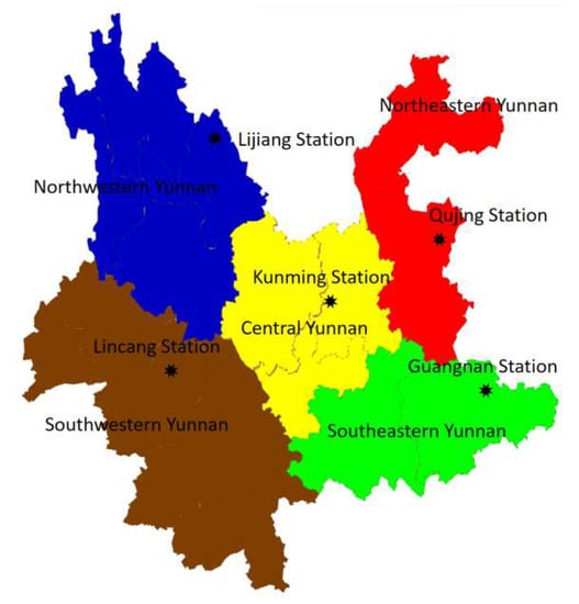
Figure 1.
Yunnan research site.
MCI was developed from the comprehensive meteorological drought index (CI) by the National Climate Center, China Meteorological Administrator [22]. The indicators were fit for real-time meteorological drought monitoring and the history of the same period meteorological drought assessment, which was calculated as
where, SPIW60 is a normalized weighted precipitation index for the past 60 days; MI30 is the relative wetness index for the last 30 days; SPI90 and SPI150 denote the standardized precipitation index for the 90-day time scale and 150-day time scale, respectively. The values of a, b, c, and d are weighting coefficients added to each calculation factor, which depend on the meteorological conditions of the study area, the calculations of these coefficients are complex, they are just tools to measure the strength of drought, so the details of them will not be given for the reason of simplifying the length of article; Ka is the value of seasonally adjusted coefficients depending on the sensitivity of crops to soil moisture in different seasons. The meteorological drought classes of the MCI drought index are computed as shown in Table 1.

Table 1.
Drought classification of MCI index.
2.3. Methods
2.3.1. Pearson Analysis of Potential Predictors
Pearson analysis is a statistical method used to measure the correlation between variables and has a wide application in data analysis and prediction [23]. Correlation coefficients take values between −1 and 1, with a higher absolute value indicating a stronger correlation. This correlation coefficient is generally expressed as r. For two time series of X and Y, its Pearson correlation coefficient is calculated as
where and are the means of the data, and r is the Pearson correlation coefficient.
For the extraction of potential predictors from the probable predictors, correlations between MCI and sixteen candidate variables were individually calculated. The variables with high correlation (Table 2) were identified and selected as predictors.

Table 2.
Correlation analysis results of candidate predictors.
The identification and selection of predictors in the development of drought prediction models are important steps for the accurate prediction of droughts. According to the results of Table 2, nine predictors are chosen including precipitation, relative humidity, 10 m wind speed, peak sunshine hours, evaporation, runoff, convective available potential energy, surface runoff, and subsurface runoff. What is more, the previous MCI data also acts as a predictor which contains information on the persistence of drought. The time series of predictors of the past five months were also used as the input of our deep learning model and the MCI for the next three months was set as the label values (i.e., the dependent variable). The predictor time series were standardized using the Z-score method to conform to a normal distribution [24]. The training set, the validation set, and the test set accounted for 60%, 20% and 20% of the dataset, respectively.
2.3.2. The Development and Application of GRU–CNN
GRU was introduced by Chung, J. et al. in 2014 as an alternative solution to ease the complexity of LSTM units. It has fewer trainable parameters because it has no output layer of LSTM. GRU is a variant of the long short-term memory (LSTM) network with a simplification and improvement of the latter [25]. GRU introduces a gating mechanism that synthesizes forgetting and input gates into an update gate with a forgetting function. GRU also mixes cell states and hidden states and adds some other modifications to solve the problems of missing long-term memory and gradient in the backpropagation of LSTM [26]. Its structural diagram is shown in Figure 2.
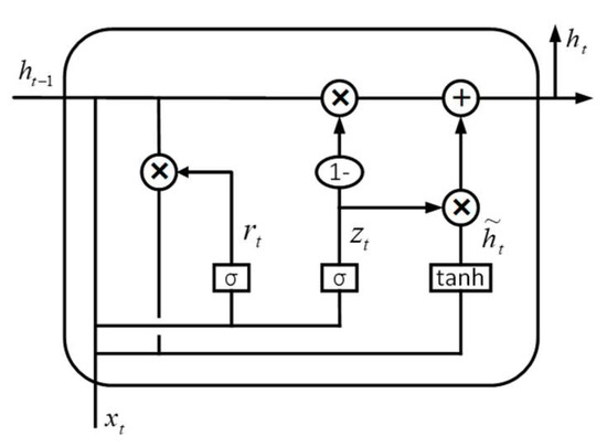
Figure 2.
Structure of GRU model.
In the figure, ht−1 is the hidden state at the moment, and xt is the input at the moment, and the reset gate output rt and the update gate output zt are calculated as follows.
where is the sigmoid activation function, wxr and wxz are the weight relations between xt and rt and zt, respectively, while whr and whz are the weight relations between ht−1 and rt and zt, respectively, and the corresponding bias terms rt and zt are denoted by br and bz, respectively [25].
The candidate state h˜t at the current moment is calculated by
where wxh and whh are the weight relationships between h˜t and xt and ht−1, bh is the corresponding bias terms, and is the vector element products. The final output ht is calculated as [27].
GRU simplifies the structure of LSTM. Compared with LSTM, the training parameters of GRU are greatly reduced, and during the training process, the latter converges faster than the former, and its training efficiency is substantially improved [28].
CNN is a kind of deep neural network and is widely used in computer vision. The pioneering work of CNN is LeNet-5 proposed by LeCun [29], and its real outbreak stage is that AlexNet won the championship in the classification task of the ImageNet competition in 2012, and the classification accuracy rate is far higher than the classification results achieved by traditional methods. It mainly consists of a convolutional layer, pooling layer, and fully connected layer. The convolutional layer is the core component of the CNN and consists of one or more convolutional kernels. Every kernel is a matrix of learnable parameters whose size is generally taken as odd numbers, such as 3 × 3 or 5 × 5. The operation process of convolution is shown in Figure 3.
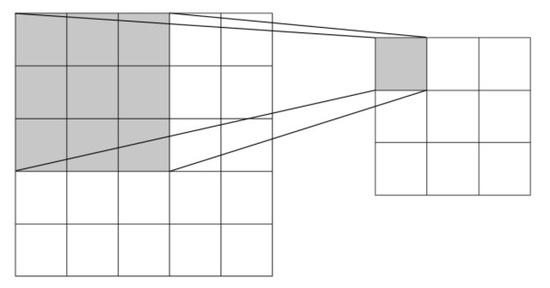
Figure 3.
Convolution operation process of the CNN model.
As can be seen from the figure, the convolution kernel is scanned row-by-row over the height and width of the image, and the convolution between the convolution kernel and the input image matrix is calculated to finally obtain the spatial characteristics of the image matrix, and the formula for the convolution operation is as follows:
where represents the value of the i-th row and j-th column of the output matrix of the convolutional layer, o is the input matrix of the convolutional network, w is a convolutional kernel matrix of the size , and represents the bias value of the i-th row and j-th column of the l-th layer.
The pooling layer is often spliced behind the convolutional layer and is a network structure first proposed by Lecun et al. [29]. Pooling layers can preserve features while simplifying the data. The most commonly used pooling operation at this stage is maximum pooling, as shown in Figure 4.
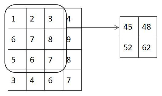
Figure 4.
Maximum pool process of the CNN model.
In the above figure, the left side is the input data with a size of 4 × 4 and the solid line box is the convolution kernel with a size of 3 × 3. It can be seen that, after maximum pooling, the amount of data is greatly reduced, but the features of the data are preserved, and such an operation can effectively reduce the number of parameters and prevent the model from overfitting [30]. The processed data are computed by the fully connected layer and then input into the activated function (ReLU for regression or Softmax for classification).
The PSO algorithm, was first proposed by Kenndy and Eberhart in 1995. The algorithm simulates the foraging behavior of birds and fish organisms in nature, and in essence, imitates the mechanism of group search to find the optimal solution to the problem [31]. Particle swarm algorithms are widely used in the current fields of path planning and numerical optimization because of a low number of parameters, a simple structure of the constructed model and uncomplicated background knowledge, and ease of operation and implementation. The relevant formulas of the particle swarm algorithm are as follows.
where is the number of iterations; and denote the exact dimensional coordinates and migration of the i-th particle at the t-th iteration, respectively; is the inertia weight; denotes the part optimal solution of the i-th particle at the t-th iteration; denotes the global optimal solution at the t-th iteration; and and are the learning factors [32]. In this paper, this factor is taken as 2; and are random numbers between 0 and 1.
To increase the convergence speed and effect of the algorithm, the inertia weights were improved in this paper so that they gradually become smaller with the increase in the number of iterations to allow the model to better converge to the global optimum, which is calculated as follows.
where is the value of at the t-th iteration; and are the maximum and minimum values of inertia weights set, respectively, and 0.9 and 0.4 were taken for both in this paper; is the maximum number of iterations, which was set to 50 in this paper.
In summary, we combined the GRU and CNN model to obtain the deep data features. The approved PSO algorithm was employed to optimize the hyper-parameters of this model including the number of hidden nodes in the first and second layers of the GRU, the number and size of convolutional kernels of the CNN.
2.4. Model Building and Experiments
To predict the MCI drought index in the Yunnan province, a novel GRU–CNN model fused with the modified PSO algorithm was proposed. The input data were the predictor time series of the past five months with a dimension of , and the MCI drought indices of the next three months acted as the label and target values to be predicted with a dimension of . Firstly, the pre-processed time series of the predictors were fed into the GRU unit to extract the temporal features. Secondly, the CNN module was used to extract the deep local features. The CNN module was composed of a two-layer CNN network and a fully connected layer. The structure diagram of the model is shown in Figure 5.
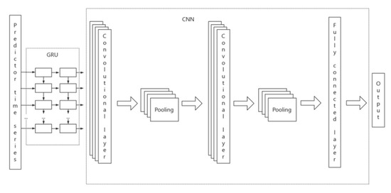
Figure 5.
Structure diagram of GRU–CNN model.
After the setup of the CNN–GRU model, its hyper-parameters were tuned using the PSO algorithm. The optimization process of the model hyper-parameters is shown in Figure 6, and the overall initial hyper-parameter settings of the GRU–CNN model based on the PSO algorithm are shown in Table 3.
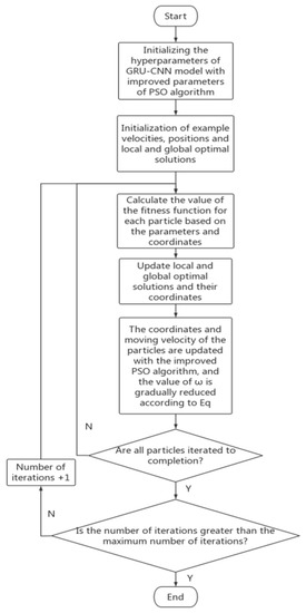
Figure 6.
Hyperparameters optimization process of the improved PSO algorithm.

Table 3.
Initial hyper-parameter settings of the GRU–CNN model based on the PSO algorithm.
For comparison with our GRU–CNN model with hyper-parameter tuning using the modified PSO algorithm, three machine learning methods were run including the least absolute shrinkage and selection operator (LASSO) [33], random forest (RF) [34] model and a GRU model with its hyper-parameters tuned with the PSO algorithm. LASSO and RF are two traditional machine learning methods and have been developed rapidly in subsequent improvements and have the advantages of low training difficulty and strong generalization ability and are widely used in regression prediction. The hyper-parameter settings of the LASSO and RF models are shown in Table 4. The GRU model was ran with its parameter settings and hyper-parameter tuned the same as our GRU–CNN model.

Table 4.
Hyper-parameter settings of the LASSO and RF.
2.5. Evaluation Metrics
The mean absolute error (MAE), root mean square error (RMSE), and Nash–Sutcliffe efficiency coefficient (NSE) [35] were used to test the predictive effect of the model, many articles have used them as the measures to evaluate the performance of models proposed [25,26,30], the three formulas are calculated as follows.
where is the number of data, is the observed value, and is the predicted value; is the Nash–Sutcliffe efficiency coefficient, refers to the observed value at time , refers to the simulated value at time , and refers to the average of the observed values. The more the Nash–Sutcliffe efficiency coefficient tends to 1, the higher the credibility of the model, and when the Nash–Sutcliffe efficiency coefficient tends to negative infinity infinitely, the lower the credibility of the model is indicated.
3. Results
The deep learning model (Figure 5) was set with the initial hyper-parameters in Table 3 and then ran as shown in Figure 6. With the same data set, we also carried out prediction experiments with LASSO, RF and GRU. The prediction skills for the MCI drought indices with first, second and third months leading are shown in Table 5, Table 6 and Table 7.

Table 5.
Performance of MCI drought index prediction models computed in the 1st month in the future.

Table 6.
Performance of MCI drought index prediction models computed in the 2nd month in the future.

Table 7.
Performance of MCI drought index prediction models computed in the 3rd month in the future.
As shown in Table 5, Table 6 and Table 7, the GRU–CNN model outperformed all other methods (LASSO, RF, and GRU) under the MEA, RMSE, and NSE metrics. As the simplest method, the LASSO was used here as the baseline. RMSE is widely used to measure the skill of regression modeling. From the average of five stations, compared with LASSO, RF and GRU, GRU–CNN reduced their RMSE by 36–41%, 71–74% and 86–88% in turn (average). RF was much better than LASSO with a 36–41% reduction and the GRU was much better with a 54–56% reduction. However, GRU–CNN exceeded GRU with a 51–54% reduction. These methods also showed a similar difference in MAE. The GRU–CNN model also held the maximum NS.
As we all know, drought is a very complex, nonlinear and cumulative climate phenomenon. As a result, the sequence of time series of predictors plays a key role in drought prediction, which means a great challenge to the regression technique. LASSO has the lowest skill because it is a simple and linear method. RF can deal with complex nonlinear problems and shows better skills than LASSO. GRU is a powerful method to compute the cumulative effect and does better than the previous two machine learning methods. The GRU–CNN model introduces the CNN module to extract the deep part features of the predictors and then gains the highest skills.
The superiority of the model has been demonstrated by the above tables (Table 5, Table 6 and Table 7). Then, we used the combined model to predict the MCI for the five selected stations. In Figure 7, Figure 8 and Figure 9, we show the prediction effect of the different models with Lincang station as an example. Other stations had similar effects, which are not shown here to save space.
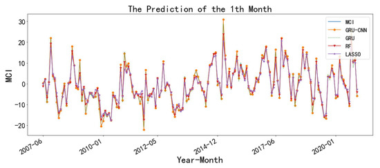
Figure 7.
The prediction of the MCI at the Lincang station with 1-month leading.
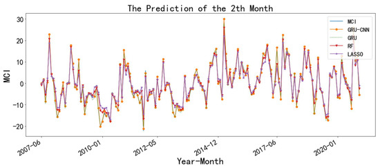
Figure 8.
The prediction of the MCI at the Lincang station with 2-month leading.
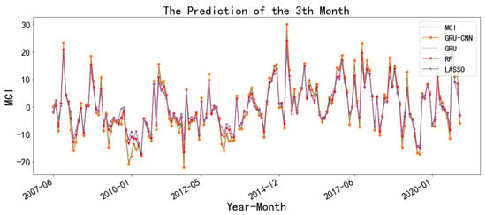
Figure 9.
The prediction of the MCI at the Lincang station with 3-month leading.
As an accumulation effect in water shortage, the predictability of drought is much lower than surface temperature and precipitation in nature. As a result, accurate prediction of drought index is a great challenge. Meanwhile, the reliable prediction of drought classification [23] (i.e., abnormally dry, moderate drought, severe drought, extreme drought) that is based on the rating of the drought index is very valuable in disaster-risk management. The experiments of prediction of drought classification were carried out to compare the ability of the above methods. Figure 10 shows the prediction skills of the different prediction models in this paper for the drought classification (computed with MCI) of the Lincang station for the next three months. The conclusion was similar to that of the drought index, where the two deep learning models significantly outperformed the machine learning models, and the GRU–CNN model further performed better than the GRU model.
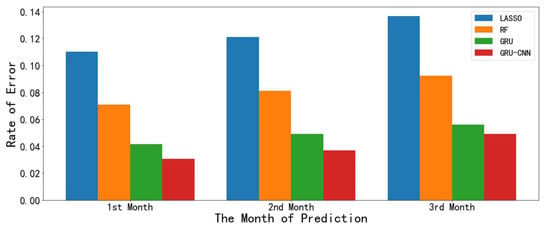
Figure 10.
The average rate of error in the prediction of drought classification in the next three months at LinCang.
4. Discussion and Conclusions
(1) Machine learning is a powerful and widely used technique for predictive modeling. However, on the condition of big data, deep learning is considered a better solution. At present, many studies have been carried out in drought prediction with machine learning methods and simple deep learning models. In this paper, an improved deep learning model was introduced by combining a gated recurrent neural network (GRU) and a convolutional neural network (CNN) with hyper-parameters tuned with an improved PSO algorithm. This model was employed to predict the meteorological composite index (MCI) for the next three months at representative stations in the Yunnan province and was compared with two traditional machine learning methods and a simple deep learning method.
(2) Both the deep learning GRU model and the GRU–CNN model significantly outperformed the traditional machine learning methods (LASSO and random forest) in the drought index prediction. This is because drought is an accumulation effect of precipitation and water shortage. The deep learning model containing a recurrent neural network such as GRU can excel in similar problems, while LASSO and random forest usually cannot perform well, thus showing lower predictive skills.
(3) The GRU–CNN model was a much more effective method in the prediction of the drought index in Yunnan province. It had reduced error (RMSE) by about half compared to the present GRU model. The CNN module is a useful tool to extract the deep local features and interrelationship of predictors so that the introduction of the CNN module can bring significant improvement to the original GRU model.
(4) Because of the above reasons, the proposed model gained more powerful abilities to deal with the complexities of time series predictions, such as the MCI drought index. The performance of the evaluation results has demonstrated the correctness of the institution of theories.
The Limitations
Although the proposed GRU–CNN model does have advantages compared with traditional models, there are still some defects that cannot be ignored in the present research:
(1) The selection and identification of predictors are very important steps for accurate prediction of droughts. The predictors selected in this paper are only based on local data. Due to the complex and diverse environment in Yunnan province, the climate there is affected by large-scale elements, such as El Niño–Southern Oscillation [36], North Atlantic oscillation, and Pacific Decadal Oscillation [37]. Although the absence of these large-scale climate elements does not hurt the value of our idea in this model, their introduction will improve the upper limit of the prediction skills of the model and should be considered in future work.
(2) Drought is complex and this research only covers the prediction of the drought index MCI of Yunnan province. A range of timescales with stable frequencies of drought including onset, severity, area, and duration of droughts are valuable for climate-risk management. Moreover, the spatial extent of drought and how this evolves was not been taken into account either. From this perspective, there are many works to do in the future.
In summary, the GRU–CNN model optimized with the improved PSO algorithm proposed in this paper can significantly improve the regression prediction of monthly drought index and the prediction of drought class based on the MCI compared with the traditional machine learning models represented by LASSO, random forest and the basic recurrent neural network deep learning model. Further study and implications of this idea will improve the prediction of drought indices and similar regression prediction studies.
Author Contributions
Conceptualization, P.M. and J.L. (Jiahui Liu); methodology, J.L. (Jiahui Liu); software, J.L. (Jiahui Liu); validation, P.M., J.L. (Jiahui Liu) and C.L.; formal analysis, P.M., J.L. (Jiahui Liu) and C.L.; investigation, P.M., J.L. (Jiahui Liu), C.L. and J.L. (Jiannan Liu); resources, P.M., J.L. (Jiahui Liu), C.L. and J.L. (Jiannan Liu); data curation, P.M., J.L. (Jiahui Liu), C.L. and J.L. (Jiannan Liu); writing—original draft preparation, P.M., J.L. (Jiahui Liu) and C.L.; writing—review and editing, P.M., J.L. (Jiahui Liu) and C.L.; visualization, J.L. (Jiahui Liu); supervision, P.M. and C.L.; project administration, P.M. and C.L.; funding acquisition, P.M. and C.L. All authors have read and agreed to the published version of the manuscript.
Funding
This research was funded by the National Key Research and Development Plan of China grant number (2017YFC1502306).
Institutional Review Board Statement
Not applicable.
Informed Consent Statement
Not applicable.
Data Availability Statement
National Climate Center: http://ncc-cma.net/cn/ (accessed on 6 November 2022).
Conflicts of Interest
The authors declare no conflict of interest.
References
- Zhang, B.; Tian, J.; Song, H.; Ma, P. Harm of agrometeorological disasters to agriculture and defense strategies. Nanfang Agric. Mach. 2019, 50, 76. (In Chinese) [Google Scholar]
- Hammer, G.L.; Hansen, J.W.; Phillips, J.G.; Mjelde, J.W.; Hill, H.; Love, A.; Potgieter, A. Advances in application of climate prediction in agriculture. Agric. Syst. 2001, 70, 515–553. [Google Scholar] [CrossRef]
- Dai, A. Increasing drought under global warming in observations and models. Nat. Clim. Change 2013, 3, 52–58. [Google Scholar] [CrossRef]
- Cheng, Q.; Gao, L.; Zhong, F.; Zuo, X.; Ma, M. Spatiotemporal variations of drought in the Yunnan–Guizhou Plateau, southwest China, during 1960–2013 and their association with large-scale circulations and historical records. Ecol. Indic. 2020, 112, 106041. [Google Scholar] [CrossRef]
- Wang, M. Research Progress on drought in Yunnan, China. Heilongjiang Agric. Sci. 2017, 122–124. [Google Scholar] [CrossRef]
- Ma, X.; Bai, S.; Huang, Y. Analysis on Drought Characteristics and drought resistance Countermeasures in Yunnan. China Rural. Water Conserv. Hydropower 2012, 101–104. (In Chinese) [Google Scholar]
- Mariotti, A.; Schubert, S.; Mo, K.; Peters-Lidard, C.; Wood, A.; Pulwarty, R.; Huang, J.; Barrie, D. Advancing drought undestangding, monitoring, and prediction. Bull. Am. Meteorol. Soc. 2013, 94, 186–188. [Google Scholar] [CrossRef]
- Kollár, A. Betting Models Using AI: A Review on ANN, SVM, and Markov Chain; MPRA Paper No. 106821; Munich Personal RePEc Archive: Munich, Germany, 2021. [Google Scholar]
- Paulo, A.A.; Pereira, L.S. Prediction of SPI drought class transitions using markov chains. Water Resour. Manag. 2007, 21, 1813–1827. [Google Scholar] [CrossRef]
- Avilés, A.; Célleri, R.; Solera, A.; Paredes, J. Probabilistic forecasting of drought events using markov chain-and bayesian network-based models: A case study of an andean regulated river basin. Water 2016, 8, 37. [Google Scholar] [CrossRef]
- Wang, Y.; Liu, J.; Wang, P.; Han, P.; Zhu, D.; Zhang, S. Research on Drought Prediction of standardized precipitation index based on Weighted Markov model. Agric. Res. Arid. Areas 2007, 25, 198–203. (In Chinese) [Google Scholar]
- Pongracz, R.; Bogardi, I.; Duckstein, L. Application of fuzzy rule-based modeling technique to regional drought. J. Hydrol. 1999, 224, 100–114. [Google Scholar] [CrossRef]
- Abdourahamane, Z.S.; Acar, R. Fuzzy rule-based forecast of meteorological drought in western Niger. Theor. Appl. Climatol. 2019, 135, 157–168. [Google Scholar] [CrossRef]
- Bardossy, A.; Bogardi, I.; Matyasovszky, I. Fuzzy rule-based downscaling of precipitation. Appl Clim. 2005, 82, 119–129. [Google Scholar] [CrossRef]
- Kinney, W.R., Jr. ARIMA and Regression in Analytical Review: An Empirical Test. Account. Rev. 1978, 53, 48–60. Available online: https://www.jstor.org/stable/245725 (accessed on 20 May 2022).
- Yeh, H.F.; Hsu, H.L. Stochastic Model for Drought Forecasting in the Southern Taiwan Basin. Water 2019, 11, 2041. [Google Scholar] [CrossRef]
- Myronidis, D.; Ioannou, K.; Fotakis, D.; Dorflinger, G. Streamflow and Hydrological Drought Trend Analysis and Forecasting in Cyprus. Water Resour. Manag. 2018, 32, 1759–1776. [Google Scholar] [CrossRef]
- Overland, J.E.; Wang, M. Large-scale atmospheric circulation changes are associated with the recent loss of Arctic sea ice. Tellus A: Dyn. Meteorol. Oceanogr. 2010, 62, 1–9. [Google Scholar] [CrossRef]
- Liao, M. Spatio-Temporal and Spatial Prediction of Rainfall in Semi-Arid Area Based on Deep Learning. Master’s Thesis, Lanzhou University, Lanzhou, China, 2021. (In Chinese). [Google Scholar]
- Liu, X.; Song, W.; Qian, F.; Wang, L.; Feng, L.; Xie, W. Meteorological drought prediction method based on vmd-cqpso-gru model. J. N. China Univ. Water Resour. Hydropower 2021, 42, 31–40. (In Chinese) [Google Scholar]
- Mi, Q.; Cao, X.; Li, Y.; Li, X.; Tang, Y.; Ren, C. Application of deep learning method to drought prediction. J. Appl. Meterogolitical Sci. 2022, 33, 104–114. [Google Scholar]
- Zhang, Q.; Xie, W.; Chen, X.; Zhai, P.; Wu, B.; Duan, J. Regional drought process and its variation characteristics in the middle-lower reaches of the Yangtze River from 1961 to 2019. Acta Meteorol. Sin. 2021, 79, 570–581. [Google Scholar]
- Cleophas, T.J.; Zwinderman, A.H. Bayesian Pearson correlation analysis. In Modern Bayesian Statistics in Clinical Research; Springer: Cham, Switzerland, 2018; pp. 111–118. [Google Scholar]
- Altman, E.I. Predicting financial distress of companies: Revisiting the Z-score and ZETA models. In Handbook of Research Methods and Applications in Empirical Finance; Bell, A.R., Brooks, C., Prokopczuk, M., Eds.; Edward Elgar Publishing: Cheltenham, UK, 2013. [Google Scholar]
- Chung, J.; Gulcehre, C.; Cho, K.; Bengio, Y. Empirical Evaluation of Gated Recurrent Neural Networks on Sequence Modeling. arXiv 2014, arXiv:1412.3555. [Google Scholar]
- Du, R. Design of Stock Trading Strategy Based on Gru Improved LSTM Gate Controlled Short-Term Memory Network. Master’s Thesis, Shanghai Normal University, Shanghai, China, 2020. (In Chinese). [Google Scholar]
- Cahuantzi, R.; Chen, X.; Güttel, S. A comparison of LSTM and GRU networks for learning symbolic sequences. arXiv 2021, arXiv:2107.02248. [Google Scholar]
- Indolia, S.; Goswami, A.K.; Mishra, S.P.; Asopa, P. Conceptual understanding of convolutional neural network- A feep learning approach. Procedia Comput. Sci. 2018, 132, 679–688. [Google Scholar] [CrossRef]
- Lecun, Y.; Bottou, L.; Bengio, Y.; Haffner, P. Gradient-based learning applied to document recognition. Proc. IEEE 1998, 86, 2278–2324. [Google Scholar] [CrossRef]
- Xu, J. Optimization and Implementation of CNN Image Recognition Algorithm Based on Zynq. Master’s Thesis, Nanjing University of Posts and Telecommunications, Nanjing, China, 2021. (In Chinese). [Google Scholar]
- Norouzi, H.; Bazargan, J. Effects of uncertainty in determining the parameters of the linear Muskingum method using the particle swarm optimization (PSO) algorithm. J. Water Clim. Change 2021, 12, 2055–2067. [Google Scholar] [CrossRef]
- Ranstam, J.; Cook, J.A. LASSO regression. J. Br. Surg. 2018, 105, 1348. [Google Scholar] [CrossRef]
- Belgiu, M.; Drăguţ, L. Random forest in remote sensing: A review of applications and future directions. ISPRS J. Photogramm. Remote Sens. 2016, 114, 24–31. [Google Scholar] [CrossRef]
- Xu, N. Research on UAV 3D path planning based on Improved PSO algorithm. Electron. Meas. Technol. 2022, 45, 78–83. (In Chinese) [Google Scholar]
- Agana, N.A.; Homaifar, A. A deep learning based approach for long-term drought prediction. In Proceedings of the SoutheastCon 2017, Concord, NC, USA, 30 March–2 April 2017; pp. 1–8. [Google Scholar]
- Özger, M.; Mishra, A.K.; Singh, V.P. Long lead time drought forecasting using a wavelet and fuzzy logic combination model: A case study in Texas. J. Hydrometeorol. 2012, 13, 284–297. [Google Scholar] [CrossRef]
- Shin, J.Y.; Kwon, H.-H.; Lee, J.-H.; Kim, T.W. Probabilistic long-term hydrological drought forecast using Bayesian networks and drought propagation. Meteorol. Appl. 2020, 27, e1827. [Google Scholar] [CrossRef]
Publisher’s Note: MDPI stays neutral with regard to jurisdictional claims in published maps and institutional affiliations. |
© 2022 by the authors. Licensee MDPI, Basel, Switzerland. This article is an open access article distributed under the terms and conditions of the Creative Commons Attribution (CC BY) license (https://creativecommons.org/licenses/by/4.0/).