Article

Evaluating the Impact of Vehicular Aerosol Emissions on Particulate Matter (PM2.5) Formation Using Modeling Study

by
Odón R. Sánchez-Ccoyllo
1,*,
Alan Llacza
2,
Elizabeth Ayma-Choque
1,
Marcelo Alonso
3,
Paula Castesana
4 and
Maria de Fatima Andrade
5
1
Escuela Profesional de Ingeniería Ambiental, Universidad Nacional Tecnologica de Lima Sur (UNTELS), Av. Bolivar S/N, Sector 3 Grupo 1, Mz. A, Sublote 3, Villa El Salvador, Lima 15834, Peru
2
National Meteorology and Hydrology Service (SENAMHI), Lima 15072, Peru
3
Faculty of Meteorology, Federal University of Pelotas, Pelotas 96001-970, RS, Brazil
4
Consejo Nacional de Investigaciones Científicas y Técnicas (CONICET), Ciudad de Buenos Aires C1425FQB, Argentina
5
Department of Atmospheric Sciences, Institute of Astronomy, Geophysics and Atmospheric Sciences, Universidade de São Paulo, São Paulo 05508-090, SP, Brazil
*
Author to whom correspondence should be addressed.
Atmosphere 2022, 13(11), 1816; https://doi.org/10.3390/atmos13111816
Submission received: 2 October 2022 / Revised: 18 October 2022 / Accepted: 24 October 2022 / Published: 1 November 2022
(This article belongs to the Section Air Quality)

Abstract

:
Automobile emissions in urban cities, such as Peru, are significant; however, there are no published studies of the effects of these emissions on PM2.5 (fine particulate matter) formation. This study aims to analyze the contributions of vehicle aerosol emissions to the surface mass concentration of PM2.5 in the Metropolitan Area of Lima and Callao (MALC), one of the most polluted cities in Latin America and the Caribbean (LAC) known to have high concentrations of PM2.5. In February 2018, we performed two numerical simulations (control and sensitivity) using the Weather Research and Forecasting model coupled with Chemistry (WRF-Chem). We considered both trace gasses and aerosol emissions from on-road traffic for the baseline simulation (hereinafter referred to as “control”); gasses without particulate emissions from vehicles were considered for the sensitivity simulation (hereinafter referred to as WithoutAerosol). For control, the model’s performance was evaluated using in situ on-ground PM2.5 observations. The results of the predicted PM2.5 concentration, temperature, and relative humidity at 2 m, with wind velocity at 10 m, indicated the accuracy of the model for the control scenario. The results for the WithoutAerosol scenario indicated that the contributions of vehicular trace gasses to secondary aerosols PM2.5 concentrations was 12.7%; aerosol emissions from road traffic contributed to the direct emissions of fine aerosol (31.7 ± 22.6 µg/m3).

1. Introduction

Exposure to high concentrations of PM2.5 (fine particulate matter having an aerodynamic diameter less than 2.5 µm) affects every organ in the human body and is associated with several diseases, including neuro-degenerative issues [1], alterations in placental genes [2], pulmonary damage [3,4], and hypertension in young people [5,6]. Sources of PM2.5 include vehicular traffic, industrial activity, energy generation, sea spray, secondary aerosol production, and dust [7,8,9]. The primary source of PM2.5 in urban cities is vehicular transport, due to the imperfect combustion of fuels, such as gasoline, diesel, and natural gas, along with emissions from non-exhaust sources, such as brake and tire wear [6,10,11,12,13,14]. Despite the importance of vehicular emissions, to date, no study so far has considered the contribution of vehicle emissions to the formation of secondary fine particles in any urban area in Peru. The city of Lima (capital city of Peru) occupies the 22nd position in the list of 40 most polluted cities in the world, based on the mean annual concentration of PM2.5 (28 µg/m3) in 2018, and the 8th position in the list of the 15 most polluted cities of the Latin America and the Caribbean (LAC) regions [15]. The Metropolitan Area of Lima and Callao (MALC) has more than 11 million inhabitants [16] over an area of 2819 km2; notably, 35% of total inhabitants of Peru live in this region, resulting in a population density of 3809.56 inhabitants/km2. The World Bank reported that the gross domestic product (GDP) per capita of Peru was USD 6958 in 2018. The MALC is a coastal city with about 2 million vehicles; this region frequently exceeds the annual Peruvian National Ambient Air Quality Standards (PNAAQS) of PM2.5 (25 µg/m3, annual mean) and World Health Organization (WHO) Air Quality Guidelines of PM2.5 (10 µg/m3, annual mean) [17]. High PM2.5 concentration from traffic emissions can reduce road visibility [18].
The weather research and forecasting coupled with chemistry (WRF-Chem) model has been applied by scholars worldwide to investigate and forecast air pollutants [19,20,21,22,23,24]. The spatio-temporal traffic emissions were calculated in Colombia by the authors of [24]. The dispersion pollutant was analyzed in a street canyon under traffic flow by the authors of [25,26]. The COPERT traffic emissions model and WRF-Chem model were coupled to simulate air pollution concentrations in Budapest, Hungary by the authors of [27]. The authors of [28] demonstrated that the average temperatures, simulated using CTMs and observed in February 2016, were higher than those observed in July 2016. Still, there are limited studies that quantify the impact of vehicular emission on the air quality of LAC using chemistry transport models (CTMs). The authors of [29] analyzed the impact of primary trace gasses on the formation of secondary particles in São Paulo, Brazil. In the MALC, there are very few applications of CTMs [30]. Therefore, new studies are needed to improve the air quality of the MALC [31].
To date, only a few studies have analyzed the sources and impacts of aerosols on human health in the MALC. Studies have shown a positive association between fine aerosol and morbidity (mainly related to respiratory and cardiovascular illnesses) in the MALC [17]. The mortality rate drop associated with decreasing PM2.5 concentration was analyzed using the AirQ+ software (version 2.0) [32]. The authors of [33] also determined the relationship between mortality due to the COVID-19 pandemic in 2020 and the PM2.5 concentration from 2012 to 2016. Consequently, several studies have been conducted on the changes in atmospheric pollution resulting from lockdown measures applied in various countries in the world, including Peru. The authors of [34] utilized the in situ ground-observed atmospheric pollutant data from 63 cities worldwide, including MALC; they demonstrated that, during the full-lockdown phase, the PM2.5 concentration declined by 43% in the MALC. PM2.5 concentrations were estimated from 2010 to 2016 using a machine learning (ML) random forest model [31]. The authors of [35] reported that the sulfate concentration in Lima in Peru was higher than that of São Paulo in Brazil and Medellin in Colombia, and according to the United States Environmental Protection Agency [36] in the MALC, more than 10,000 deaths annually can be attributed to fine particle matter exposure.
According to a report of the Asociación Automotriz del Peru (AAP, translated as the Automotive Association of Peru), in Peru, the average age of private vehicles is about 16 years old, and the average age of public vehicles is about 23 years old [37]. The ages of vehicles are old and therefore fuel consumption is poor in the MALC. According to the TomTom Traffic Index (TOM2) report, in 2018, the MALC was the third-most traffic-congested region in the world, following the cities of Mumbai in India and Bogotá in Colombia [38]. Additionally, according to the Japan International Cooperation Agency report [39], on the most important roads of the MALC, the average speed of vehicles during both the morning and night peak hours of traffic is less than 20 km/h; the cost for working hours lost because of the traffic congestion add up to USD 6750 [37].
In this study, in 2018–2019, the average, maximum, and minimum annual air temperatures in the MALC were 19.0, 31.0, and 13.2 °C, respectively, and the average, maximum, and minimum annual relative humidity was 84.0, 98.0, and 46.0%, respectively. This study was carried out in scientific collaboration with the Emissions in South America (EMiSA) network, made up of five countries from South America, and international scientists [40]. This study aims to analyze the contributions of vehicle aerosol emissions to the surface mass concentration of PM2.5 in the Metropolitan Area of Lima and Callao (MALC) in February 2018, using the air quality model WRF-Chem (version 4.0).

2. Materials and Methods

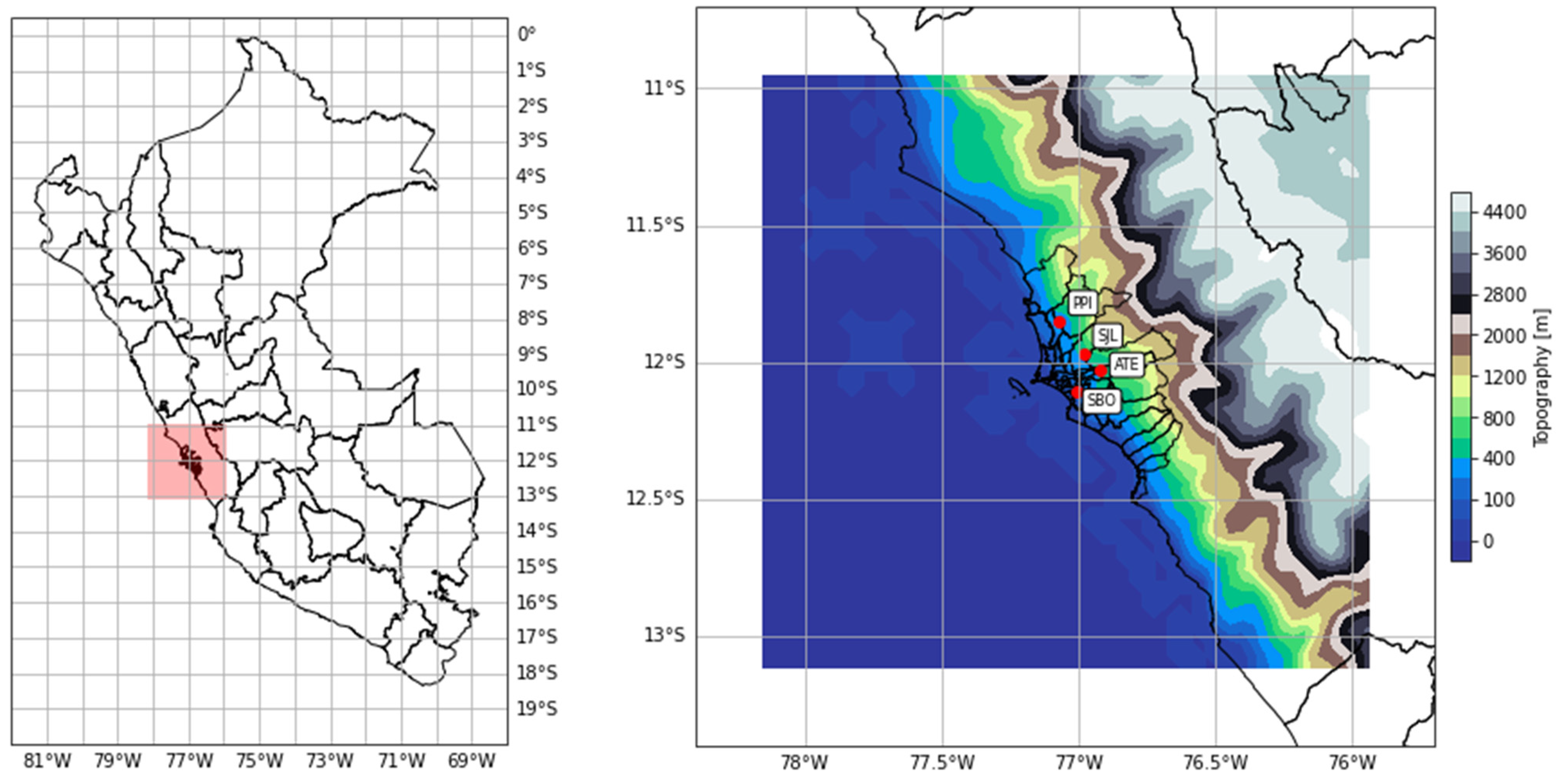
2.1. Description of Study Area and Data

In this study, for the MALC, we selected four automatic air-quality monitoring stations (AAQMS), due to the availability of the measured concentrations of PM2.5 for these stations. They were located in Ate [12°1′34″ S, 76°55′7″ W; altitude: 362 m above sea level (MASL)], San Borja (SBO) (12°6′31.06″ S, 77°0′27.96″ W; altitude: 136 MASL), San Juan de Lurigancho (SJL) (11°58′53.7″ S, 76°55′57.6″ W; altitude: 239 MASL), and Puente Piedra (PPI) (11°51′47.71″ S, 77°4′26.88″ W; altitude: 180 MASL), as shown in Figure 1. From the PPI station, there were also observations of additional meteorological variables. The Ate station, which was located in the eastern part of Lima, was characterized as the predominant source of heavy-duty vehicles and light-duty vehicles. The SBO station was located in an area where the predominant residential source was cooking, and the SJL station, also located in the eastern part of Lima, was characterized as the predominant source of light-duty vehicles and residential sources. The PPI station, located in the northern part of Lima, was characterized by commercial areas, heavy-duty vehicles, and light-duty vehicles.
The hourly concentrations of the PM2.5 data were obtained from the AAQMS operated by the National Meteorology and Hydrology Service of Peru (SENAMHI) for February 2018. Additionally, we considered the hourly measurements of air temperature at a height of 2 m (T2), relative humidity at a height of 2 m (RH2), and wind speed at a height of 10 m (WS10) that were available for the PPI AAQMS acquired from the SENAMHI for the same study period. These environmental data were used to evaluate the performance of the outputs of the WRF-Chem model for different scenarios.
According to a report by [41] for PROTRANSPORTE (Instituto Metropolitano Protransporte de Lima, translated as Metropolitan Protransport Institute of Lima), the total vehicle fleets in the MALC consisted of six vehicle types: light vehicles (47.7%), taxis (7.7%), pickup trucks (27.6%), motorcycles (1.4%), busses (3.1%), and trucks (12.3%). According to a report by the Instituto Nacional de Estadistica e Informatica (INEI; translated as “National Institute of Statistics and Informatics”), the total vehicular traffic was 72,238,205 (79%) units per year for light-duty vehicles (LDV) and 19,282,049 (21%) units per year for heavy-duty vehicles (HDV), as counted at the toll collection sites in the MALC in 2018. In addition, the total traffic volume was 91,520,254 (100%) units in 2018 in the MALC [42].

2.2. Meteorological Conditions in February 2018

On 1 February 2018, an anticyclonic circulation (ACi) was observed at 500 hPa, SW of MALC (16° S, 77° W); this ACi generated a temperature inversion, which resulted in a static stability at low atmosphere. The average air dewpoint temperature during the study period was 19.5 ± 0.6 °C. The accumulated daily precipitation on 26 February 2018, was 1.0 mm, which could be attributed to the cyclonic circulation at 850 hPa, NW of the MALC (11° S, 80° W); no precipitation occurred on the other days of February 2018. The maximum (Tmax), minimum (Tmin) air temperature measured at JCAi was 24.3–29.5 °C and 19.0–21.9 °C, respectively, while the thermal amplitude (Tmax–Tmin) was 2.8–9.4 °C (Figure 2), with relatively minor variations, due to the permanent presence of low stratus clouds over the MALC and JCAi, owing to their locations being close to the sea.

2.3. Ground-Measured PM2.5 Records: Filling Data Gaps with Machine Learning (ML)

We employed the simple linear regression (SLR) ML model to record the hourly PM2.5 measurements from the on-ground AAQMS, to predict the missing data (MID) of the PM2.5 in the four AAQMS: Ate (9.97% of MID), SBO (13.1% of MID), SJL (6.99% of MID), and PPI (6.69% of MID). The SLR was implemented in Python, using scikit-learn ML reference library, as previously applied by [43]. Notably, the SLR model was dependent on the unknown PM2.5 data-gaps predicted (target or response) from the AAQMS PM2.5 observation-data (predictor) [44]. For the test set phase of the SLR model, the training set was chosen randomly, with 80% of the available measured data acquired from the four AAQMS (487 hourly PM2.5 data) and 20% being the measured dataset (122 hourly PM2.5 data). The SLR model performed efficiently, with a mean absolute error (MAE) of 8.3 µg/m3 and RMSE (root mean square error) of 12.46 µg/m3. More details of the MAE and RMSE have been explained [45,46,47].

2.4. Weather Research and Forecasting Coupled with Chemistry (WRF-Chem) Model Description

The WRF-Chem model is a numerical model that can simulate meteorological variables and the concentrations of atmospheric pollutants simultaneously [19,48]. In this study, we applied the WRF-Chem model (version 4.0) to the entire MALC region. For the initial and boundary conditions of the WRF model, we retrieved the meteorological variables from the Global Tropospheric Analyses and Forecast Grids (GDAS/FNL), with a horizontal resolution of 0.25° × 0.25° (https://rda.ucar.edu/datasets/ds083.3/, accessed on 10 August 2020), developed by the National Center for Environmental Prediction (NCEP). We selected the following physics schemes: Purdue Lin for microphysics [49], rapid radiative transfer model for longwave radiation [50], Goddard shortwave for shortwave radiation, Noah land surface model for land surface physics, Yonsei University for planetary boundary layer scheme [51], Grell 3D scheme for cumulus parameterization [52], and four surface-soil levels for land surface; the vertical resolution was implemented using 32 levels. Further, we selected the vegetation and land-use types of classifications based on the 24-category data of the United States Geological Survey (USGS) [53]. The topography was retrieved from the advanced spaceborne thermal emission and reflection radiometer-global digital elevation Model (ASTER GDEM). The resolution of the WRF-Chem model was 5 × 5 km; this model domain surrounded the MALC with 50 (W − E) × 50 (S − N) grids, as suggested by [30].
In this study, the gas-phase chemical reactions were considered using the regional acid deposition model (RADM2) chemical mechanism, while the aerosol reactions were considered using the modal aerosol dynamics model for Europe (MADE) combined with the secondary organic-aerosol model (SORGAM). For the preparation of boundary conditions for chemical analysis, an idealized profile was used, such as the one used by [19], for gas species and aerosols, respectively. We incorporated the dry deposition, according to the authors of [48]. The parameterizations of this model for the control case are consolidated in Table 1. The predictions were established to run from 30 January 2018 to 2 March 2018; the run for 30–31 January 2018 was considered for the spin-up of the model to reduce the effects of the initial chemical and meteorological conditions. In this study, the WRF dynamical core selected the Advanced Research WRF (ARW) model to run an ARW simulation. We used Eulerian nonhydrostatic equations, Arakawa C-grid staggering, and three-dimensional for real data, and adaptive time step (adjusted based on the Courant-Friedrichs-Lewy condition), simple diffusion, and positive-definite advection for moisture. The format of the input, history, restart, and boundary files are netCDF format. We selected the dry deposition of gas species and aerosols, no biomass burning emissions, no Goddard Chemistry Aerosol Radiation and Transport aerosol module (GOCART) dust emissions, no GOCART Dimethyl Sulfate (DMS) emissions from the sea surface, and no feedback from the aerosols to radiation schemes; emissions were speciation for RADM2/SORGAM.

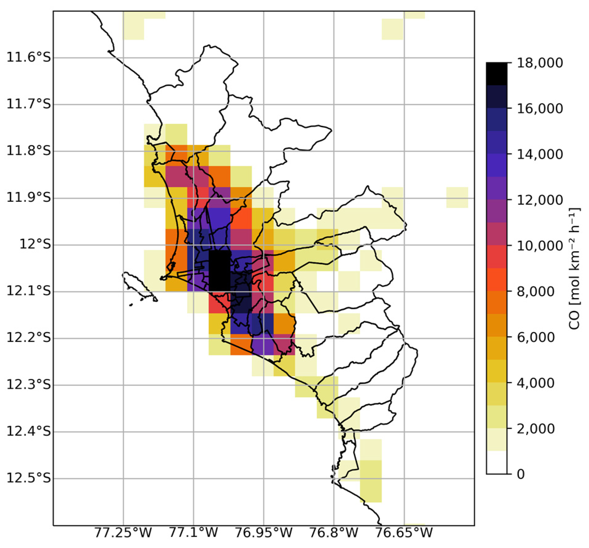
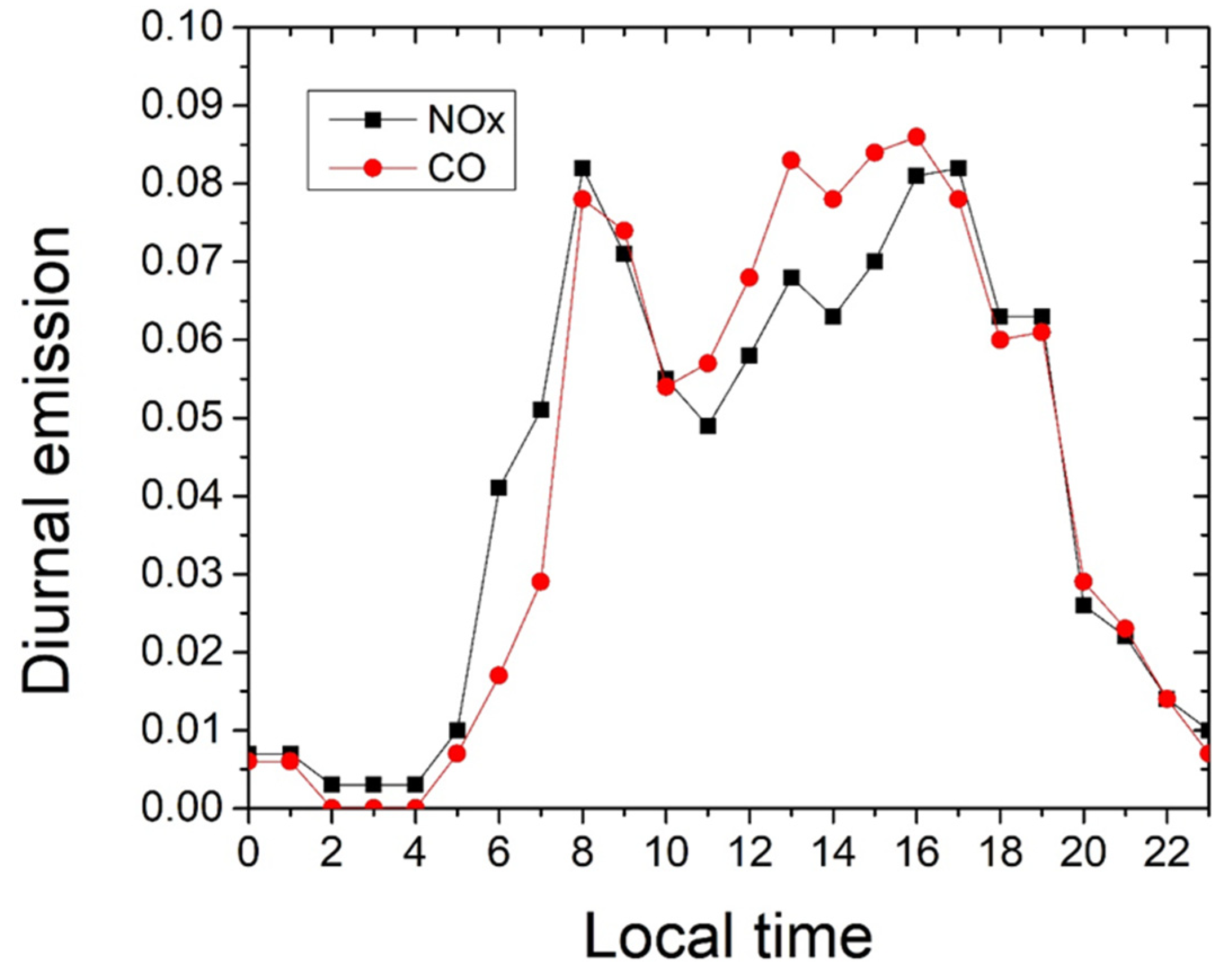
2.5. Anthropogenic Vehicle Emissions in the Metropolitan Area of Lima and Callao (MALC)

We calculated the total vehicle emissions in the MALC using the motor vehicle emissions model established by [54]. In general, this method requires three parameters from ground transportation (mobile emission factor, number of vehicles, and the distance (km) covered by vehicles per day for each type of vehicle). Therefore, the total emissions of CO, SO2, volatile organic compounds (VOCs), PM2.5, PM10, NO2, and NO were input as the vehicle emissions data in each grid cell, obtained using Equation (1) [55], as follows:
VE = Num * EF * VKTr
where,
VE = vehicle emissions (g/day),
Num = number of vehicles,
EF = mobile emission factor (g/km), and
VKTr = vehicle kilometer travel per day for each type of vehicle (km/day).
The EF and VKTr data for Equation (1) were obtained from [41]; the EF data was for six vehicle types (motorcycles, buses, trucks, pickup trucks, LDV, and taxis) for the following pollutants: CO, NOx, particulate matter, SO2, and VOCs.
Subsequently, we carried out the distribution of the spatial disaggregation of anthropogenic mobile emissions (CO, NOx, particulate matter, SO2, and VOCs), based on a mass-conserving emissions preprocessor [29,56] with the horizontal resolution of the grid cells being 5 × 5 km (see Figure 3); the spatial distributions were based on the traffic emissions approach [54], while assuming that the total vehicle numbers were distributed proportionate to the road’s length, for each grid cell of 5 × 5 km. The road information was systematized by the OpenStreetMap data (https://www.openstreetmap.org/relation/288247, accessed on 19 July 2021) and retrieved freely from the Geofabrik website (https://www.geofabrik.de/, accessed on 21 July 2021), in accordance with [29,54].
The hourly variations in the mobile ground emissions data in each grid cell in the WRF-Chem model are based on the temporal profile of [57] was used (Figure 4). In addition, the temporal variations in the data for LDV could be mostly attributed to the CO emissions and those in the data for HDV could be mostly attributed to the NOx emissions [58].
The spatiotemporally allocated emissions were utilized as input for the WRF-Chem model, as previously applied by [24]. Notably, in this study, we considered only automobile emission inventories, e.g., previous works of [29,54], because according to a report of the Ministerio del Ambiente del Peru (MINAM, translated as the Ministry of Environment of Peru), the primary source of air pollution in the MALC is vehicular transport, accounting for 89% of the total emissions [59].

2.6. Statistical Metrics Approach to Evaluate the Model Performance

We evaluated the output of the meteorological variables predicted by the WRF-Chem model by comparing the output data with the hourly measurements data of the meteorological variables (ground temperature, surface relative humidity, and wind speed) acquired from the SENAMHI (available for the PPI station). These simulated hourly meteorological variables were evaluated using the following statistical techniques: mean bias (MB), RMSE, and mean gross error (MGE), in accordance Appendix A with [60,61,62]. Air temperature at a height of 2 m above the ground, relative humidity at a height of 2 m above the ground, and wind speed at a height of 10 m above the ground were measured hourly using the automatic meteorological monitoring system operated by the SENAMHI.
The performance of the model to predict the PM2.5 concentrations was evaluated using the statistical approach proposed by [63], including the determination of the mean fractional bias (FraB) and mean fractional error (FraE), with the recommended criteria being −60% ≤ FraB ≤ 60% and FraE ≤ 75%. At the PPI, SBO, and Ate stations, the hourly PM2.5 concentrations were measured 3 m above the ground, while at the SJL station, the hourly PM2.5 concentrations were measured 6 m above the ground, using the Thermo Scientific Model 5014i Beta, which is automatic equipment that utilizes Beta ray attenuation, at each of the four AAQMSs operated by the SENAMHI.

2.7. Sensitivity Tests

To evaluate the impact of aerosol vehicular emissions on PM2.5 concentrations in the MALC, we considered two vehicle emissions in the WRF-Chem (version 4.0) model: (i) simulations of hourly measurements of air pollutants and meteorological variables were carried out for both vehicular emission gasses and aerosols, which was used as the simulation control case, hereinafter referred to as “Control”, to evaluate the performance of the model; (ii) simulations of vehicular gas emissions, without considering vehicular aerosol-emissions, hereinafter referred to as “WithoutAerosol,” were employed to evaluate the contribution of vehicular aerosol emissions to the surface concentration of PM2.5. The differences between the results of the Control and WithoutAerosol simulations were considered as the impact of vehicular aerosol emissions on the PM2.5 formations in the MACL; this numerical simulation was adapted from previous works [29,56,64].

3. Results and Discussion

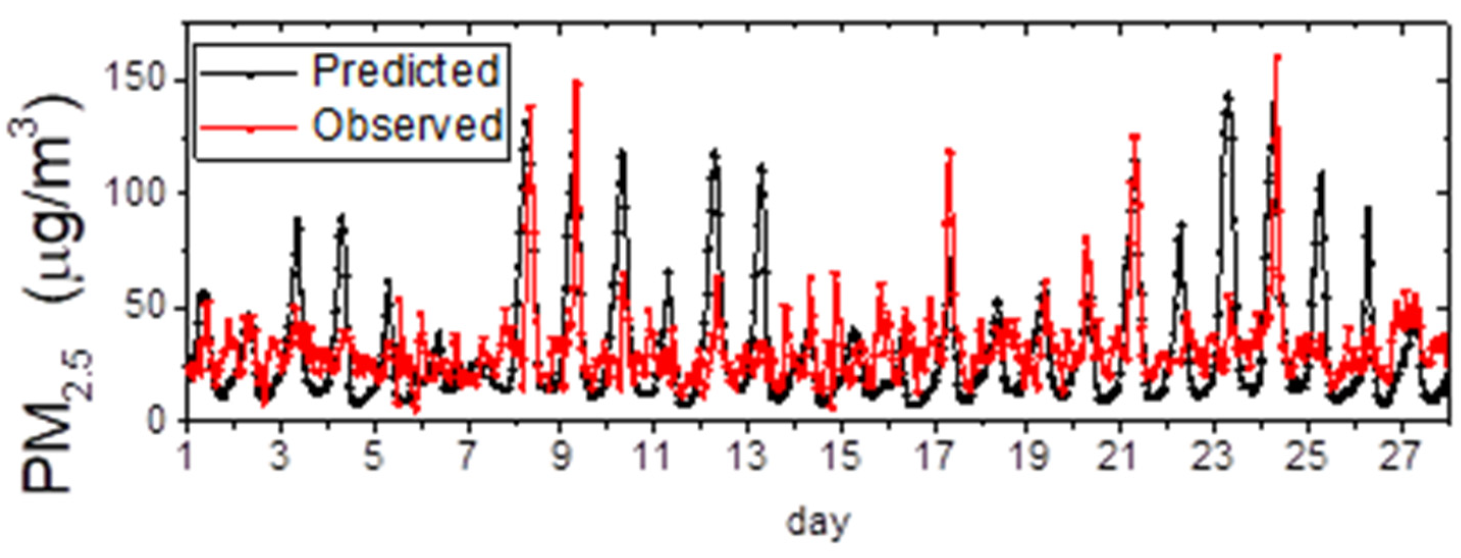
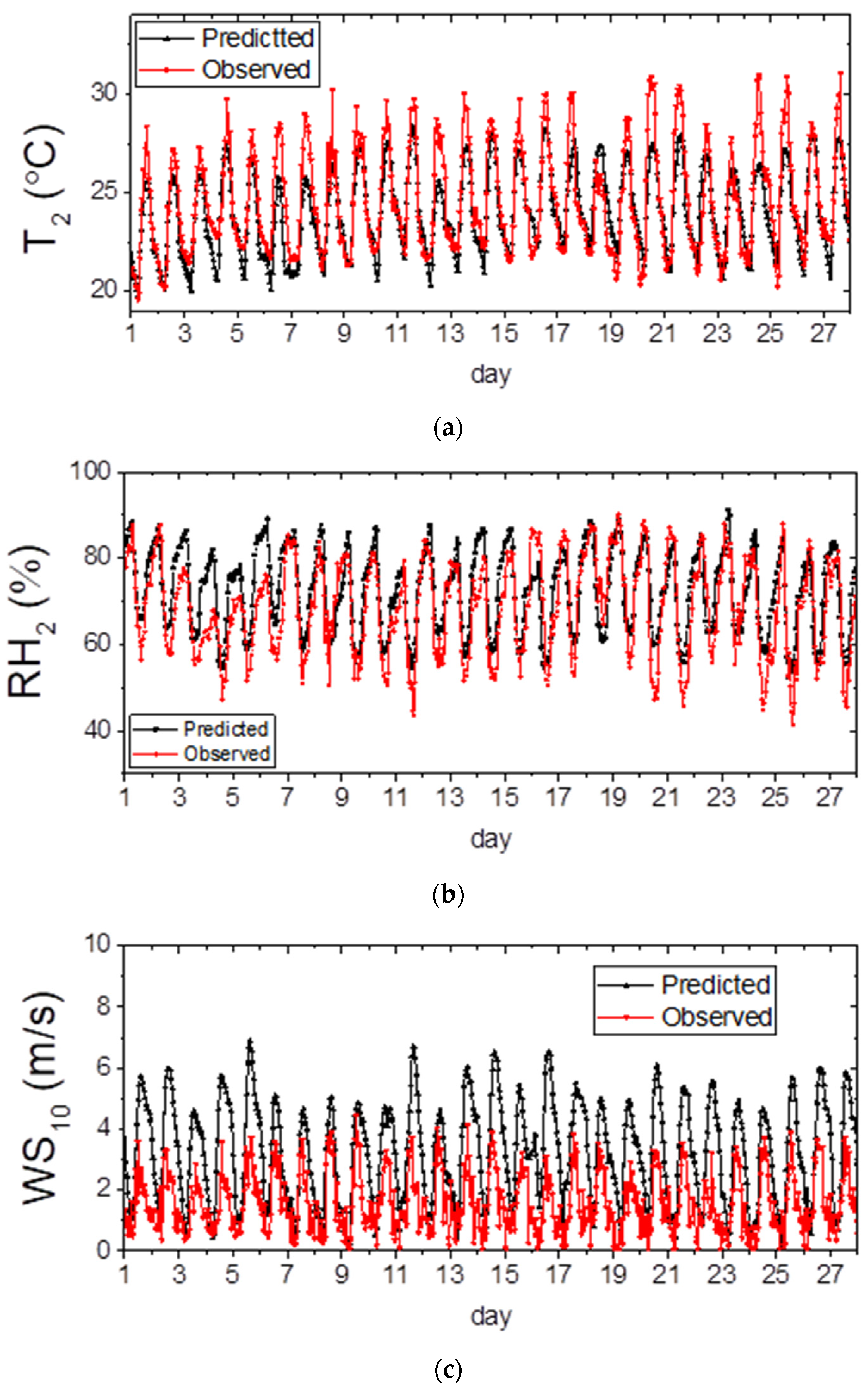
3.1. Evaluation of Model Performance in Terms of Determining PM2.5 Concentration and Meteorological Variables

As shown in Figure 5, we compared the results of the simulations of the hourly concentrations of PM2.5 obtained using the WRF-Chem model for the control case simulation (Control) and those measured at Ate AAQMS for February 2018. The hourly temporal variation simulations of PM2.5 concentrations captured the fine aerosol hourly temporal variations in the observed PM2.5 in Ate (Figure 5). At this station, the measured hourly PM2.5 concentrations were 5–160 µg/m3, whereas the predicted hourly PM2.5 concentrations were 7–143 µg/m3 (Figure 5).
The results of the WRF-Chem model for control portrayed four AAQMSs in the MALC, namely, Ate, SBO, SJL and PPI; we used the FraB and FraE metrics, as per the criteria suggested by [63], to enable the model to accurately predict the PM2.5 concentrations for the different stations (Table 2). The statistical indicators of the accuracy of the WRF-Chem model were comparable with previous works [65].
In Figure 6, we showed a comparison between the measured and simulated hourly air temperature data at a height of 2 m (T2), measured and simulated hourly relative humidity data at a height of 2 m (RH2), and hourly wind speed measured and simulated data at a height of 10 m (WS10) for February 2018 in the MALC. The model slightly underestimated the T2 data, compared to the observed data (Figure 6a). In addition, the simulated maximum temperatures were a little lower than the measured values. Hourly temperature (T2 data) and simulated maximum temperature were slightly lower than their measured temperatures. This may be due to the fact that the sensible heat flux (SHF) simulated with the WRF model was slightly lower than the SHF measured in Metropolitan Lima, whereas the measured and simulated minimum temperatures were similar for most of the time series during the study period (Figure 6a). The diurnal variations in the observed RH2 were well-captured by the WRF-Chem model (Figure 6b). The diurnal variations in the high values of the measured hourly RH2 data were also accurately simulated by the model. The RMSE of RH2 at PPI was 7.05% (Table 3), which is smaller than other values calculated in other studies, such as one conducted in China, the authors of [66] calculated an RMSE of 12.7% for RH2. The authors of [67] calculated an RMSE of 16.60% for RH2. In this study, the hourly WS10 values simulated by the WRF-Chem model was overpredicted (Figure 6c). Another previous study has also proven that the WRF-Chem model overpredicts the WS10 values [62,68,69,70,71].
Table 3 portrays the model performance in determining the meteorological variables for Lima. The air temperature was slightly underpredicted. The MB of the temperature was −0.57 °C. The mean gross error (MGE) of the temperature was 1.05 °C, which was less than the benchmark (≤2.0 °C) applied by [68]. The measured and simulated average temperatures during the study period were 24.6 ± 2.7 °C and 24.0 ± 2.1 °C, respectively, which were close; therefore, we could conclude that the WRF-Chem model was effective in simulating the temperature for the study area, with an RMSE error of 1.38 °C (Table 3). The measured and simulated average relative humidity values were 68.7 ± 11.1% and 72.4 ± 9.6%, respectively, which confirmed that the relative humidity was overestimated by the MB value of 3.63% that met the benchmark of RH2 (≤±10%) applied by [65]; the MGE was 5.86%, which met the benchmark of RH2 (≤20%) applied by [65], and RH2 portrayed an RMSE simulation error of 7.05% (Table 3). However, for China, the authors of [71] underpredicted the RH2, with MB = −7.3%. In this study, the wind velocity was overpredicted; the MB of wind velocity was 1.66 m/s. The MGE of wind velocity was 1.72 m/s, which was below the benchmark (≤2.0 m/s) applied by [68]. The RMSE of wind velocity was 2.05 m/s.

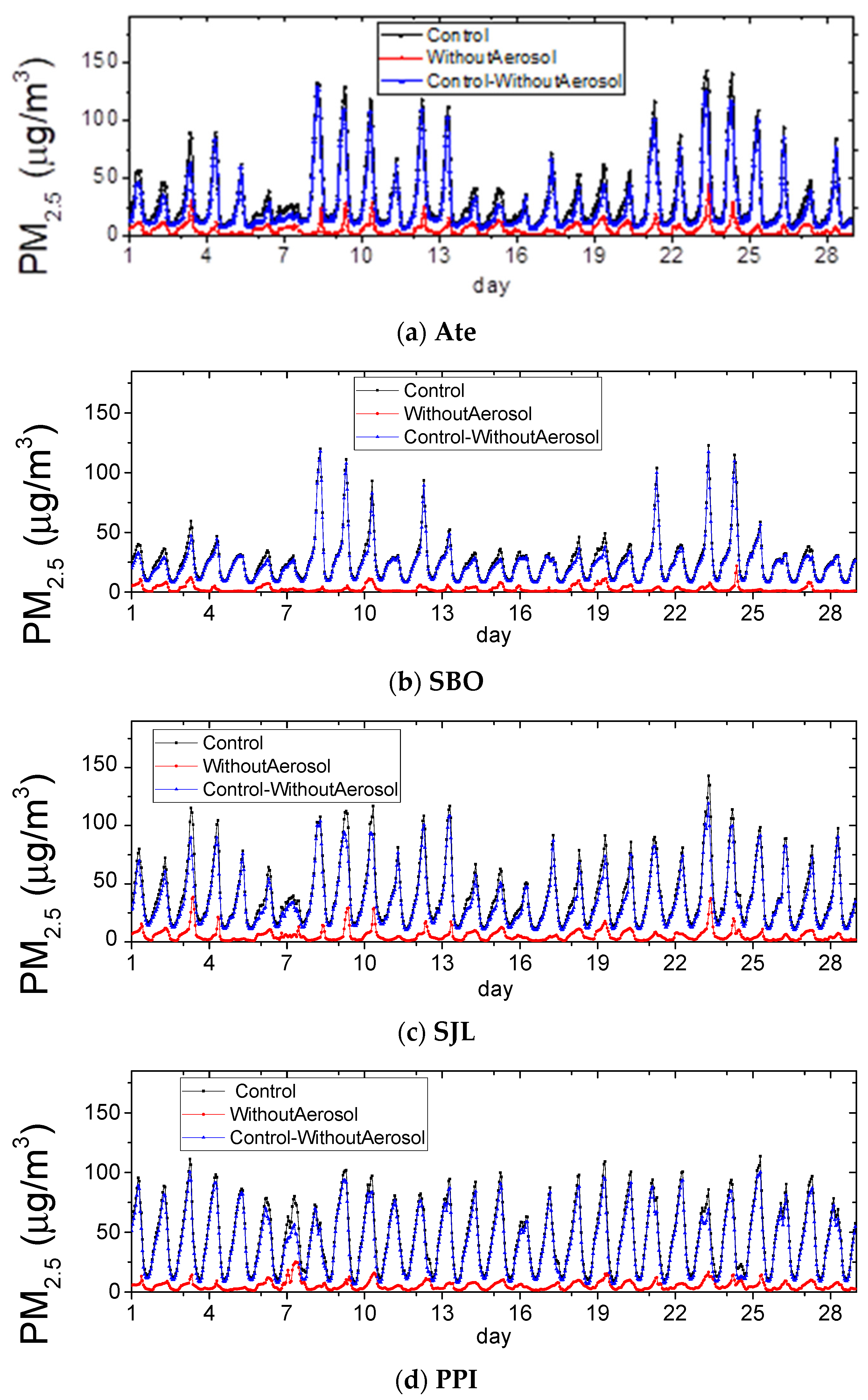
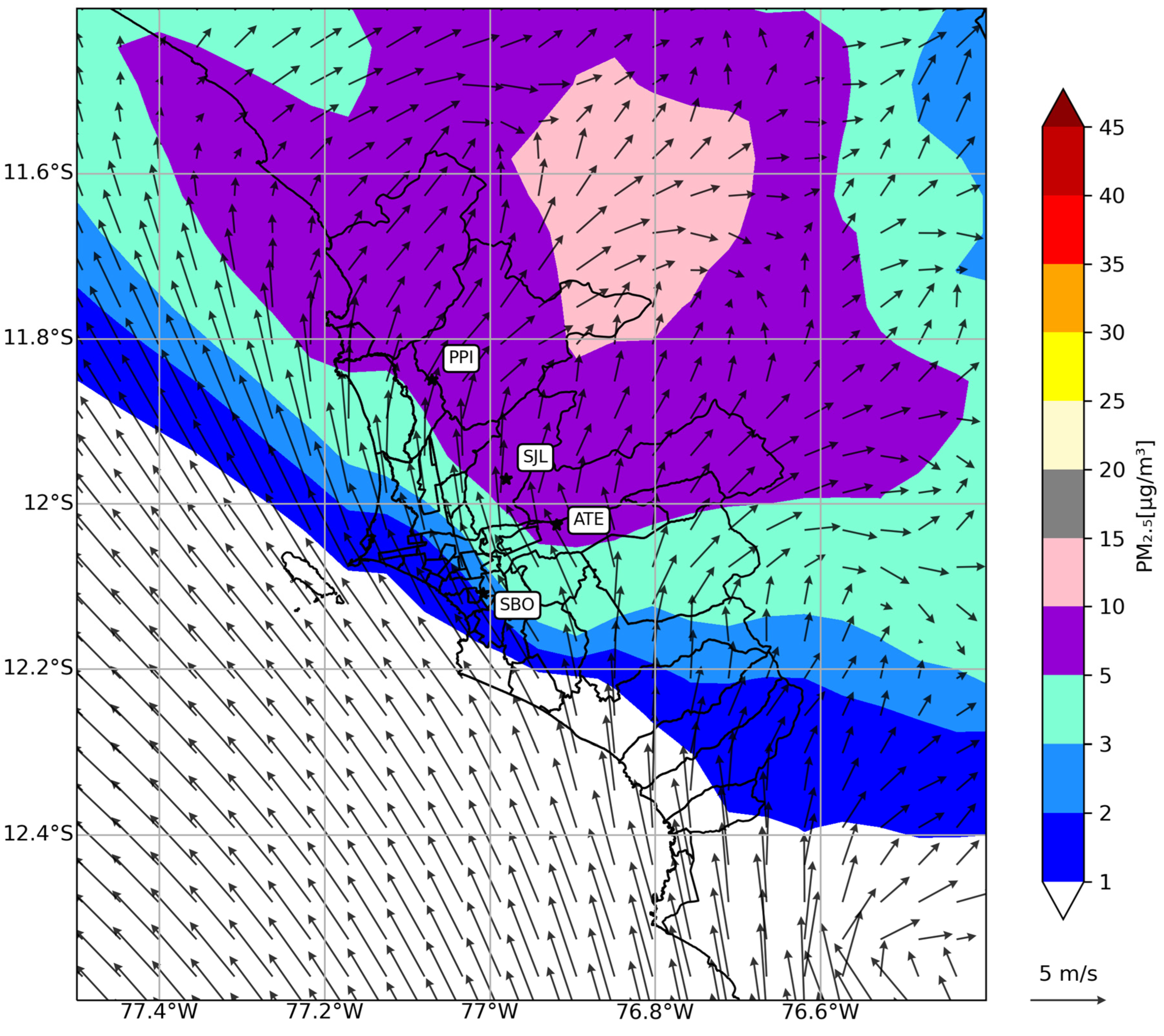
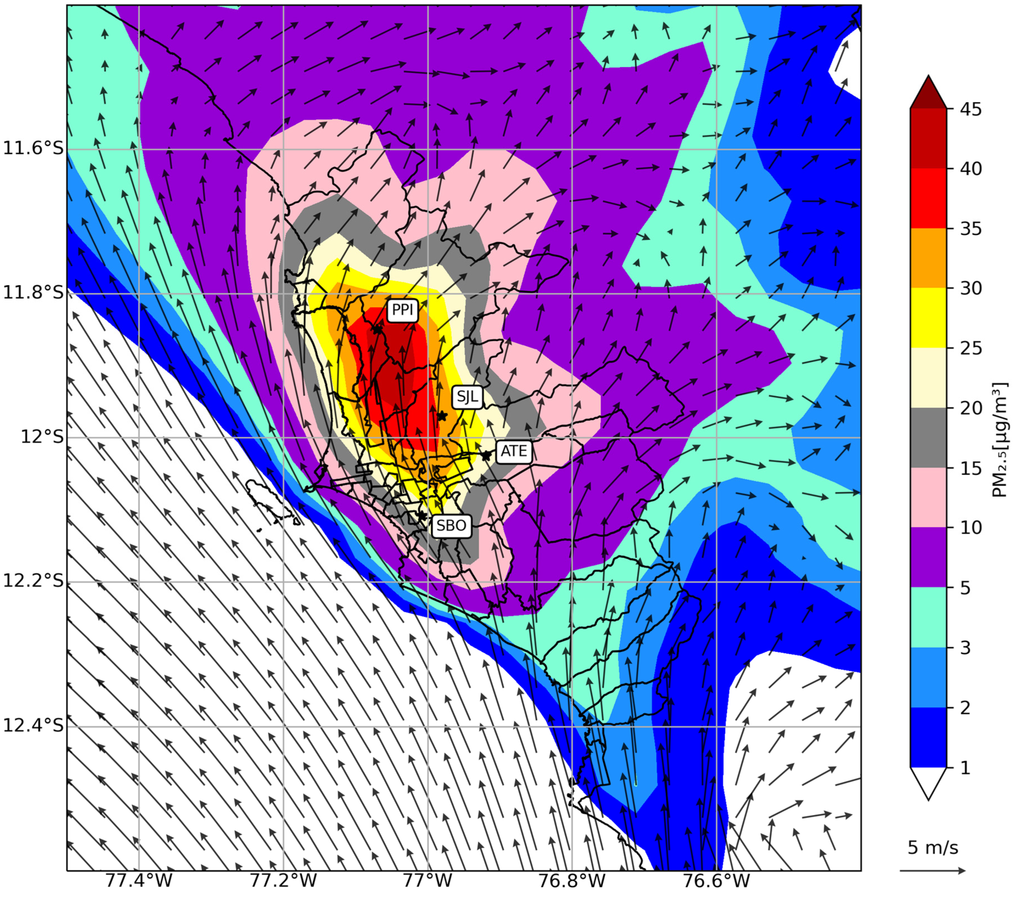
3.2. Effect of Vehicular Aerosol Emission on PM2.5 Formation

Figure 7 portrays a comparison of the hourly time series for February 2018 between the control and WithoutAerosol scenarios, with the difference between the control and WithoutAerosol (Control-WithoutAerosol) results indicating the impacts of vehicle aerosol emissions on the formation of PM2.5 in the four AAQMSs considered in this study in the MALC. First, at the Ate AAQMS, the hourly values of the impact of transport aerosol emissions on the hourly formation of PM2.5 were 6–128 µg/m3, whereas the hourly values of the control scenario were 7.4–142.8 µg/m3 (Figure 7a); in terms of the hourly values for the entire month of February for the WithoutAerosol scenario, the vehicular gas emissions added to the formations of fine aerosol were 16.9% of the total PM2.5. Second, for the SBO AAQMS, the contribution of vehicular aerosol emissions to the hourly formation of PM2.5 was 7.5–117.7 µg/m3 (Figure 7b); the hourly levels for the control scenario varied from 8.1 µg/m3 to 122.9 µg/m3 (Figure 7b). Third, for SJL AAQMS, the vehicular aerosol emissions contributed 10.4–119.1 µg/m3 to the hourly formation of PM2.5 (Figure 7c). Fourth, for the PPI AAQMS, the contribution of transport aerosol emission to the hourly formation of PM2.5 was 6.4–100.5 µg/m3; however, the hourly values for the control scenario were 8.5–113.6 µg/m3 (Figure 7d). Considering the four AAQMSs mentioned above, the results of the WRF-Chem model indicated that the impact of vehicular aerosol emissions on the formation of the maximum hourly PM2.5 and in terms of the hourly values for the entire month of February for the (Control-WithoutAerosol) scenario of PM2.5 contributed 128.2 µg/m3 and (31.7 ± 22.6 µg/m3) to the formations of secondary fine aerosols, respectively. In addition, the impact of primary-gas automobile emissions could be attributed to the formation of secondary particles of PM2.5, with 12.7% of the total PM2.5 mass concentrations compared to the control scenario in February 2018.
Figure 8 portrays a spatial distribution of the mean monthly PM2.5 concentrations for the control scenario during February 2018. For the Ate AAQMS, the simulated PM2.5 concentrations was 20–25 µg/m3; for SBO station, the simulated PM2.5 concentrations varied from 15–20 µg/m3. For SJL AAQMS, the simulated PM2.5 concentrations were 30–40 µg/m3; in addition, for PPI AAQMS, the simulated PM2.5 concentration was 45 µg/m3. The mean simulated values for PM2.5 concentration for the control in all study areas of the MALC were 15–45 µg/m3. Moreover, the prevailing wind direction during our study period was from the south of the MALC; therefore, low concentrations of PM2.5 remain in the southern regions of Lima and high values were simulated for the northern regions of Lima, such as PPI (Figure 8).
Figure 9 portrays the spatial distribution of the simulated average monthly PM2.5 concentrations for February 2018 for the WithoutAerosol simulation performed using the WRF-Chem model. In the WithoutAerosol simulation at the SBO station, the contributions of gaseous-phase emissions from vehicles to formations of secondary fine particles ranged from 1 µg/m3 to 2 µg/m3. For the other three AAQMS (Ate, SJL, and PPI), in the WithoutAerosol simulation, the contributions of vehicle gas emissions to the formation of secondary fine aerosols ranged from 5 µg/m3 to 10 µg/m3. Additionally, the values of the WithoutAerosol in the MALC noted that the contributions of secondary fine particles ranged from 1 µg/m3 to 10 µg/m3, with low values of mean monthly PM2.5 observed in the southern region of the MALC, and high values observed in the northern and eastern regions of the MALC. The highest values of the simulated mean monthly PM2.5 for WithoutAerosol in the study area were located NE of the MALC (11.65° S; 76.8° W); the plume observed from 10 µg/m3 to 15 µg/m3 may indicate the PM2.5 formations transported to the peak plume by the wind blowing from the SW direction (Figure 9).
Figure 10 portrays the spatial distribution of the impact of vehicle aerosol emissions on PM2.5 formation for February 2018. The contributions of automobile aerosol emissions ranged from 15 µg/m3 to 20 µg/m3 at the AAQMSs of Ate and SBO, respectively. For the SJL site, the contribution of vehicular aerosol emissions to the formation of secondary particles varied from 30 µg/m3 to 40 µg/m3. For PPI, the formation of PM2.5 ranged from 40 µg/m3 to 45 µg/m3. In addition, the impact of road-traffic aerosol emissions contributed to the formation of secondary PM2.5 particles, ranging from 15 µg/m3 to 45 µg/m3 in the MALC during the total investigation period. The high PM2.5 values were observed in the northern regions of the MALC, such as PPI; the PM2.5 particles were transported from the central and southern regions of Lima to the northern part of Lima by the wind, with the wind being blown from the southern direction (Figure 10).

4. Conclusions

Although the important role of road-traffic transport emissions for local environments is well established, there is a lack of evidence regarding the effects of fine atmospheric aerosol (PM2.5) emissions from automobiles. Furthermore, such studies have not been conducted in Peru. The aim of this study was to analyze the contributions of vehicle aerosols emissions to surface mass concentration of PM2.5 in the MALC megacity.
We carried out two numerical simulations using the CTM named WRF-Chem model (version 4.0). First, we applied the control simulation (control), in which we performed atmospheric environmental simulations. We used the WRF-Chem model and considered both primary gas and aerosol emissions from automobiles. Two statistical techniques, the FraB and FraE, were applied to validate the predicted PM2.5 concentrations, using the in situ PM2.5 data observed on the ground. Second, a model sensitivity simulation was applied, which considered the same control simulation, without the emissions of aerosols from vehicles (WithoutAerosol). The simulations of the PM2.5 concentrations for the control examination met the precision criteria of the model because the FraB and FraE values met the criteria for PM2.5 recommended by [63]. The simulations of air temperature, relative humidity, and wind speed for the control examination met the accuracy criteria of the model, as the MGE and RMSE results met the accuracy criteria applied by [65]. The WithoutAerosol scenario portrayed that the vehicular gas emissions contributed to the formation of the secondary particles of PM2.5 concentrations significantly (12.7%), compared to the control scenario; however, the impact of aerosol emissions from road traffic was attributable to the formation of secondary fine aerosol (31.7 ± 22.6 µg/m3).
Future studies must perform vertical measurements of atmospheric pollutants, mainly in the planetary boundary layer of the atmosphere of the urban cities in Peru, to validate the vertical simulations using the WRF-Chem model.

Author Contributions

Conceptualization, O.R.S.-C. and M.d.F.A.; methodology, O.R.S.-C. and M.d.F.A.; software, A.L.; validation, O.R.S.-C.; data curation, E.A.-C.; writing—original draft preparation, O.R.S.-C.; writing—review and editing, M.d.F.A., E.A.-C., A.L., M.A. and P.C. All authors have read and agreed to the published version of the manuscript.

Funding

This research was funded by CONCYTEC-FONDECYT now ProCIENCIA, grant number 424-2019-FONDECYT and this study was developed by the Universidad Nacional Tecnológica de Lima Sur (UNTELS) under the contract 424-2019-FONDECYT.

Institutional Review Board Statement

Not applicable.

Informed Consent Statement

Not applicable.

Data Availability Statement

The WRF-Chem model (version 4.0) model used in this study can be found here: https://www2.mmm.ucar.edu/wrf/users/download/get_source.html accessed on 17 May 2022. For the initial and boundary conditions of the WRF model, we retrieved the meteorological variables from the Global Tropospheric Analyses and Forecast Grids (GDAS/FNL), with a horizontal resolution of 0.25° × 0.25° are available at https://rda.ucar.edu/datasets/ds083.3/ accessed on 17 May 2022.

Acknowledgments

We would like to thank Lara Schwars from the University of California, USA, for their valuable insights pertaining to the revision of this manuscript. We would like to thank the anonymous reviewers that gave us interesting suggestions to improve the article.

Conflicts of Interest

The authors declare no conflict of interest.

Acronyms

ACi, Anticyclonic circulation; AAP, Asociación Automotriz del Peru; CTM, chemistry transport models; EMiSA, Emissions in South America; FE, mobile factor emissions; LAC, Latin America and the Caribbean regions; LT, local time; MAE, mean absolute error; MB, mean bias; FraB, mean fractional bias; FraE, mean fractional error; MGE, mean gross error; MALC, Metropolitan Area of Lima and Callao; MID, missing data; MADE, modal aerosol dynamics model for Europe; RAMD2, regional acid deposition model; RMSE, root mean square error; SORGAM, secondary organic-aerosol model; SLR, simple linear regression; USEPA, United States Environmental Protection Agency; USGS, United States Geological Survey; VOCs, volatile organic compounds; WRF-Chem, Weather Research and Forecasting coupled with chemistry; K, The horizontal (Kh) and vertical (Kv) eddy viscosities.

Appendix A

The formulas for statistical model evaluation used in this study are described below:
  • Mean bias (MB):
M B = 1 N k = 1 N ( A k O k )
2.
Root mean square error (RMSE):
R M S E = k = 1 N ( A k O k ) 1 N
3.
Mean Gross Error (MGE):
M G E = 1 N k = 1 N | A k O k | O k × 100
4.
Fractional bias (FraB):
F r a B = 2 N k = 1 N ( A k O k ) ( A k + O k ) × 100
5.
Fractional error (FraE):
F r a E = 2 N k = 1 N | A k O k | ( A k + O k ) × 100
6.
Mean absolute error (MAE):
M A E = 1 N k = 1 N | A k O k |
where Ak and Ok are the predicted and observed PM2.5 and meteorological variables, respectively, and N is the hourly PM2.5 concentration or meteorological variables observed-predicted pairs.

References

  1. Cristaldi, A.; Fiore, M.; Conti, G.; Pulvirenti, E.; Favara, C.; Grasso, A.; Copat, C.; Ferrante, M. Possible association between PM2.5 and neurodegenerative diseases: A systematic review. Environ. Res. 2022, 15, 112581. [Google Scholar] [CrossRef] [PubMed]
  2. Kaur, K.; Lesseur, C.; Deyssenroth, M.A.; Kloog, I.; Schwartz, J.D.; Marsit, C.J.; Chen, J. PM2.5 exposure during pregnancy is associated with altered placental expression of lipid metabolic genes in a US birth cohort. Environ Res. 2022, 211, 113066. [Google Scholar] [CrossRef] [PubMed]
  3. Wen, J.; Chuai, X.; Gao, R.; Pang, B. Regional interaction of lung cancer incidence influenced by PM2.5 in China. Sci Total Environ. 2022, 10, 149979. [Google Scholar] [CrossRef]
  4. Guo, X.; Lin, Y.; Lin, Y.; Zhong, Y.; Yu, H.; Huang, Y.; Yang, J.; Cai, Y.; Liu, F.; Li, Y.; et al. PM2.5 induces pulmonary microvascular injury in COPD via METTL16-mediated m6A modification. Environ. Pollut. 2022, 303, 119115. [Google Scholar] [CrossRef]
  5. Liang, X.; Chen, J.; An, X.; Liu, F.; Liang, F.; Tang, X.; Qu, P. The impact of PM2.5 on children’s blood pressure growth curves: A prospective cohort study. Environ. Int. 2022, 1, 107012. [Google Scholar] [CrossRef] [PubMed]
  6. Li, J.; Dong, Y.; Song, Y.; Dong, B.; Martin, R.; Shi, L.; Ma, Y.; Zou, Z.; Ma, J. Long-term effects of PM2.5 components on blood pressure and hypertension in Chinese children and adolescents. Environ. Int. 2022, 161, 107134. [Google Scholar]
  7. Siudek, P. Seasonal distribution of PM2.5-bound polycyclic aromatic hydrocarbons as a critical indicator of air quality and health impact in a coastal-urban region of Poland. Sci. Total Environ. 2022, 827, 154375. [Google Scholar] [CrossRef]
  8. Yang, J.; Kang, S.; Ji, Z.; Tripathee, L.; Yin, X.; Yang, R. Investigation of variations causes and component distributions of PM2.5 mass in China using a coupled regional climate-chemistry model. Atmos. Pollut. Res. 2020, 11, 319–331. [Google Scholar]
  9. Liu, W.; Xu, Y.; Liu, W.; Liu, Q.; Yu, S.; Liu, Y.; Wang, X.; Tao, S. Oxidative potential of ambient PM2.5 in the coastal cities of the Bohai Sea, northern China: Seasonal variation and source apportionment. Environ. Pollut. 2018, 236, 514–528. [Google Scholar] [CrossRef]
  10. Tofful, L.; Canepari, S.; Sargolini, T.; Perrino, C. Indoor air quality in a domestic environment: Combined contribution of indoor and outdoor PM sources. Build. Environ. 2021, 202, 108050. [Google Scholar] [CrossRef]
  11. Pinto, J.A.; Kumar, P.; Alonso, M.F.; Andreão, W.L.; Pedruzzi, R.; Santos, F.S.; Moreira, D.M.; Albuquerque, T.T.A. Traffic data in air quality modeling: A review of key variables, improvements in results, open problems and challenges in current research. Atmos. Pollut. Res. 2020, 11, 454–468. [Google Scholar] [CrossRef]
  12. Andrade, M.F.; Kumar, P.; Freitas, E.D.; Ynoue, R.Y.; Martins, J.; Martins, L.D.; Nogueira, T.; Perez-Martinez, P.; Miranda, R.M.; Albuquerque, T.; et al. Air quality in the megacity of São Paulo: Evolution over the last 30 years and future perspectives. Atmos. Environ. 2017, 159, 66–82. [Google Scholar] [CrossRef]
  13. Ibarra-Espinosa, S.; Ynoue, R.Y.; Ropkins, K.; Zhang, X.; Freitas, E.D. High spatial and temporal resolution vehicular emissions in south-east Brazil with traffic data from real-time GPS and travel demand models. Atmos. Environ. 2020, 222, 117136. [Google Scholar] [CrossRef]
  14. Soleimani, M.; Akbari, N.; Saffari, B.; Haghshenas, H. Health effect assessment of PM2.5 pollution due to vehicular traffic (case study: Isfahan). J. Transp. Health 2022, 24, 101329. [Google Scholar] [CrossRef]
  15. IQAir. 2018 World Air Quality Report Region and City PM2.5 Ranking [Internet]. 2018 [Cited 2021 Jul 17]. Available online: https://www.iqair.com/world-air-quality-ranking (accessed on 18 July 2021).
  16. City Population. All Urban Agglomerations of the World with a Population of 1 Million Inhabitants or More [Internet]. 2022 [Cited 2022 Jan 2]. Available online: https://citypopulation.de/en/world/agglomerations/ (accessed on 3 January 2022).
  17. Tapia, V.; Steenland, K.; Sarnat, S.E.; Vu, B.; Liu, Y.; Sánchez-Ccoyllo, O.; Vasquez, V.; Gonzales, G.F. Time-series analysis of ambient PM2.5 and cardiorespiratory emergency room visits in Lima, Peru during 2010–2016. J. Expo. Sci. Environ. Epidemiol. 2020, 30, 680–688. [Google Scholar]
  18. Luo, L.; Bai, X.; Liu, S.; Wu, B.; Liu, W.; Lv, Y.; Guo, Z.; Lin, S.; Zhao, S.; Hao, Y.; et al. Fine particulate matter (PM2.5/PM1.0) in Beijing, China: Variations and chemical compositions as well as sources. J. Environ. Sci. 2022, 121, 187–198. [Google Scholar] [CrossRef]
  19. Grell, G.A.; Peckham, S.E.; Schmitz, R.; McKeen, S.A.; Frost, G.; Skamarock, W.C.; Eder, B. Fully coupled ‘online’ chemistry within the WRF model. Atmos. Environ. 2005, 39, 6957–6975. [Google Scholar] [CrossRef]
  20. Jat, R.; Gurjar, B.R.; Lowe, D. Regional pollution loading in winter months over India using high resolution WRF-Chem simulation. Atmos. Res. 2021, 249, 105326. [Google Scholar] [CrossRef]
  21. Kong, Y.; Sheng, L.; Li, Y.; Zhang, W.; Zhou, Y.; Wang, W.; Zhao, Y. Improving PM2.5 forecast during haze episodes over China based on a coupled 4D-LETKF and WRF-Chem system. Atmos. Res. 2021, 249, 105366. [Google Scholar] [CrossRef]
  22. Sati, A.P.; Mohan, M. Impact of increase in urban sprawls representing five decades on summer-time air quality based on WRF-Chem model simulations over central-National Capital Region, India. Atmos. Pollut. Res. 2021, 12, 404–416. [Google Scholar] [CrossRef]
  23. Sicard, P.; Crippa, P.; Marco, A.; Castruccio, S.; Giani, P.; Cuesta, J.; Paoletti, E.; Feng, Z.; Anav, A. High spatial resolution WRF-Chem model over Asia: Physics and chemistry evaluation. Atmos. Environ. 2021, 244, 118004. [Google Scholar] [CrossRef]
  24. Hernández, K.S.; Henao, J.J.; Rendón, A.M. Dispersion simulations in an Andean city: Role of continuous traffic data in the spatio-temporal distribution of traffic emissions. Atmos. Pollut. Res. 2022, 13, 101361. [Google Scholar] [CrossRef]
  25. Zhao, Y.; Jiang, C.; Song, X. Numerical evaluation of turbulence induced by wind and traffic, and its impact on pollutant dispersion in street canyons. Sustain. Cities Soc. 2021, 74, 103142. [Google Scholar] [CrossRef]
  26. Zheng, X.; Yang, J. CFD simulations of wind flow and pollutant dispersion in a street canyon with traffic flow: Comparison between RANS and LES. Sustain. Cities Soc. 2021, 75, 103307. [Google Scholar] [CrossRef]
  27. Kovács, A.; Leelossy, Á.; Tettamanti, T.; Esztergár-Kiss, D.; Mészáros, R.; Lagzi, I. Coupling traffic originated urban air pollution estimation with an atmospheric chemistry model. Urban Clim. 2021, 37, 100868. [Google Scholar] [CrossRef]
  28. Reátegui-Romero, W.; Sánchez-Ccoyllo, O.R.; Andrade, M.F.; Moya-Alvarez, A. PM2.5 Estimation with the WRF/Chem Model, Produced by Vehicular Flow in the Lima Metropolitan Area. Open J. Air Pollut. 2018, 7, 215–243. [Google Scholar] [CrossRef] [Green Version]
  29. Vara-Vela, A.; Andrade, M.F.; Kumar, P.; Ynoue, R.Y.; Muñoz, A.G. Impact of vehicular emissions on the formation of fine particles in the Sao Paulo Metropolitan Area: A numerical study with the WRF-Chem model. Atmos. Chem. Phys. 2016, 16, 777–797. [Google Scholar] [CrossRef] [Green Version]
  30. Sánchez-Ccoyllo, O.R.; Ordoñez-Aquino, C.G.; Muñoz, Á.G.; Llacza, A.; Andrade, M.F.; Liu, Y.; Reátegui-Romero, W.; Brasseur, G. Modeling Study of the Particulate Matter in Lima with the WRF-Chem Model: Case Study of April 2016. Int. J. Appl. Eng. Res. 2018, 13, 10129–10141. [Google Scholar] [CrossRef]
  31. Vu, B.N.; Sánchez, O.; Bi, J.; Xiao, Q.; Hansel, N.N.; Checkley, W.; Gonzales, G.F.; Steenland, K.; Liu, Y. Developing an advanced PM2.5 exposure model in Lima, Peru. Remote Sens. 2019, 11, 641. [Google Scholar] [CrossRef] [Green Version]
  32. Sánchez-Ccoyllo, O.R.; Ordoñez-Aquino, C.G.; Arratea-Morán, J.; Marín-Huachaca, N.S.; Reátegui-Romero, W. Describing aerosol and assessing health effects in Lima, Peru. Int. J. Environ. Sci. Dev. 2021, 12, 355–362. [Google Scholar] [CrossRef]
  33. Vasquez-Apestegui, B.; Parras-Garrido, E.; Tapia, V.; Paz-Aparicio, V.M.; Rojas, J.P.; Sanchez-Ccoyllo, O.R.; Gonzales, G.F. Association between air pollution in Lima and the high incidence of COVID-19: Findings from a post hoc analysis. BMC Public Health 2021, 21, 1161. [Google Scholar] [CrossRef] [PubMed]
  34. Sokhi, R.S.; Singh, V.; Querol, X.; Finardi, S.; Targino, A.C.; Andrade, M.F.; Pavlovic, R.; Garland, R.M.; Massagué, J.; Kong, S.; et al. A global observational analysis to understand changes in air quality during exceptionally low anthropogenic emission conditions. Environ. Int. 2021, 157, 106818. [Google Scholar] [CrossRef]
  35. Pereira, G.M.; Oraggio, B.; Teinilä, K.; Custódio, D.; Huang, X.; Hillamo, R.; Alves, C.; Balasubramanian, R.; Rojas, N.; Sanchez-Ccoyllo, O.R.; et al. A comparative chemical study of PM10 in three Latin American cities: Lima, Medellín, and Sao Paulo. Air Qual. Atmos. Health 2019, 12, 1141–1152. [Google Scholar] [CrossRef]
  36. USEPA. Assessing the Mortality Burden of Air Pollution in Lima-Callao [Internet]. 2021 [Cited 7 July 2022]. pp. 1–56. Available online: https://www.epa.gov/sites/default/files/2021-06/documents/lima_megacities_technical_report_20210514_english_0.pdf. (accessed on 11 April 2022).
  37. AAP. [Junk Bonos] [Internet]. 2020 [Cited 7 July 2022]. pp. 1–11. Available online: https://aap.org.pe/actualizateconlaaap/bono-chatarreo/Bono-Chatarreo.pdf (accessed on 14 January 2022).
  38. TOM2. TomTom Traffic Index: Mumbai Takes Crown of ‘Most Traffic Congested City’ in World [Internet]. 2019 [Cited 7 July 2022]. Available online: https://www.businesswire.com/news/home/20190603005831/en/TomTom-Traffic-Index-Mumbai-takes-Crown-%E2%80%98Most (accessed on 12 July 2021).
  39. JICA. [Survey to Collect Basic Information on Urban Transport in the Metropolitan Area of Lima and Callao. Final Report] [Internet]. 2013 [Cited 7 July 2022]. pp. 1–113. Available online: https://openjicareport.jica.go.jp/Pdf/12087532_01.Pdf (accessed on 28 January 2022).
  40. Huneeus, N.; Gon, D.H.; Castesana, P.; Menares, C.; Granier, C.; Granier, L.; Alonso, M.; Andrade, M.F.; Dawidowski, L.; Gallardo, L.; et al. Evaluation of anthropogenic air pollutant emission inventories for South America at national and city scale. Atmos. Environ. 2020, 235, 117606. [Google Scholar] [CrossRef]
  41. Deuman, I.; Walsh, I.C.C. Informe Final: Estudio de Línea Base Ambiental COSAC I [Internet]. Lima; 2005 [Cited 7 June 2022]. Available online: https://www.scribd.com/document/366319703/Resumen-Ejecutivo-Linea-Base-Ambiental (accessed on 6 June 2022).
  42. INEI. Transporte, Almacenamiento, Correo y Mensajería. Lima Metropolitana: Tráfico Vehicular Mensual Registrado, por Tipo de Vehículo y Centro de Recaudación-Garitas, 2011–2020 [Internet]. 2022 [Cited 30 June 2022]. Available online: https://www.inei.gob.pe/ (accessed on 1 July 2022).
  43. Lumiaro, E.; Todorović, M.; Kurten, T.; Vehkamäki, H.; Rinke, P. Predicting gas-particle partitioning coefficients of atmospheric molecules with machine learning. Atmos. Chem. Phys. 2021, 21, 13227–13246. [Google Scholar] [CrossRef]
  44. Topalović, D.B.; Davidović, M.D.; Jovanović, M.; Bartonova, A.; Ristovski, Z.; Jovašević-Stojanović, M. In search of an optimal in-field calibration method of low-cost gas sensors for ambient air pollutants: Comparison of linear, multilinear and artificial neural network approaches. Atmos. Environ. 2019, 213, 640–658. [Google Scholar] [CrossRef]
  45. Fung, P.L.; Zaidan, M.A.; Timonen, H.; Niemi, J.; Kousa, A.; Kuula, J.; Luoma, K.; Tarkoma, S.; Petäjä, T.; Kulmala, M.; et al. Evaluation of white-box versus black-box machine learning models in estimating ambient black carbon concentration. J. Aerosol. Sci. 2021, 152, 105694. [Google Scholar] [CrossRef]
  46. Pei, Z.; Zhang, D.; Zhi, Y.; Yang, T.; Jin, L.; Fu, D.; Cheng, X.; Terryn, H.A.; Mol, J.M.C.; Li, X. Towards understanding and prediction of atmospheric corrosion of an Fe/Cu corrosion sensor via machine learning. Corros. Sci. 2020, 170, 108697. [Google Scholar] [CrossRef]
  47. Yang, N.; Shi, H.; Tang, H.; Yang, X. Geographical and temporal encoding for improving the estimation of PM2.5 concentrations in China using end-to-end gradient boosting. Remote Sens. Environ. 2022, 269, 112828. [Google Scholar]
  48. Fast, J.D.; Gustafson, W.I.; Easter, R.C.; Zaveri, R.A.; Barnard, J.C.; Chapman, E.G.; Grell, G.A.; Peckham, S.E. Evolution of ozone, particulates, and aerosol direct radiative forcing in the vicinity of Houston using a fully coupled meteorology-chemistry-aerosol model. J. Geophys. Res. 2006, 16, 111. [Google Scholar] [CrossRef]
  49. Chen, S.H.; Sun, W.Y. A One-dimensional Time Dependent Cloud Model. J. Meteorol. Soc. Jpn. 2002, 80, 99–118. [Google Scholar] [CrossRef] [Green Version]
  50. Mlawer, E.J.; Taubman, S.J.; Brown, P.D.; Iacono, M.J.; Clough, S.A. Radiative transfer for inhomogeneous atmospheres: RRTM, a validated correlated-k model for the longwave. J. Geophys. Res. 1997, 102, 16663–16682. [Google Scholar] [CrossRef] [Green Version]
  51. Hong, S.Y.; Noh, Y.; Dudhia, J.A. New Vertical Diffusion Package with an Explicit Treatment of Entrainment Processes. Mon. Weather Rev. 2006, 134, 2318–2341. [Google Scholar] [CrossRef] [Green Version]
  52. Grell, G.A.; Dévényi, D. A generalized approach to parameterizing convection combining ensemble and data assimilation techniques. Geophys. Res. Lett. 2002, 29, 38-1–38-4. [Google Scholar] [CrossRef]
  53. Li, H.; Zhang, H.; Mamtimin, A.; Fan, S.; Ju, C.A. new land-use dataset for the weather research and forecasting (WRF) Model. Atmosphere 2020, 11, 350. [Google Scholar] [CrossRef] [Green Version]
  54. Andrade, M.F.; Ynoue, R.; Freitas, E.D.; Todesco, E.; Vela, A.V.; Ibarra, S.; Martins, L.D.; Martins, J.A.; Carvalho, V.S.B. Air quality forecasting system for Southeastern Brazil. Front. Environ. Sci. 2015, 3, 9. [Google Scholar] [CrossRef] [Green Version]
  55. Zhang, Q.; Tong, P.; Liu, M.; Lin, H.; Yun, X.; Zhang, H.; Tao, W.; Liu, J.; Wang, S.; Tao, S.; et al. A WRF-Chem model-based future vehicle emission control policy simulation and assessment for the Beijing-Tianjin-Hebei region, China. J. Environ. Manag. 2020, 253, 109751. [Google Scholar] [CrossRef]
  56. Vara-Vela, A.; Andrade, M.F.; Zhang, Y.; Kumar, P.; Ynoue, R.Y.; Souto-Oliveira, C.E.; Silva, L.F.J.; Landulfo, E. Modeling of Atmospheric Aerosol Properties in the São Paulo Metropolitan Area: Impact of Biomass Burning. J. Geophys. Res. Atmos. 2018, 123, 9935–9956. [Google Scholar] [CrossRef]
  57. Lents, J.; Davis, N.; Nikkila, N.; Osses, M. Lima Vehicle Activity Study. Final Report [Internet]. 2004 [Cited 7 July 2022]. Available online: http://www.gssr.net/ (accessed on 21 January 2022).
  58. Liu, Y.; Huang, W.; Lin, X.; Xu, R.; Li, L.; Ding, H. Variation of spatio-temporal distribution of on-road vehicle emissions based on real-time RFID data. J. Environ. Sci. 2022, 116, 151–162. [Google Scholar] [CrossRef]
  59. MINAM. El Perú y el Cambio Climático, Segunda Comunicación Nacional del Perú (Traslated as “Peru and Climate Change, Second National Communication of Peru”) [Internet]. Lima; 2010, [Cited 7 July 2022]. Available online: http://www.minam.gob.pe (accessed on 8 April 2022).
  60. Chuang, M.T.; Wu, C.F.; Lin, C.Y.; Lin, W.C.; Chou, C.C.K.; Lee, C.T.; Lin, T.H.; Fu, J.S.; Kong, S.S.K. Simulating nitrate formation mechanisms during PM2.5 events in Taiwan and their implications for the controlling direction. Atmos. Environ. 2022, 269, 118856. [Google Scholar] [CrossRef]
  61. Wang, X.; Li, L.; Gong, K.; Mao, J.; Hu, J.; Li, J.; Liu, Z.; Liao, H.; Qiu, W.; Yu, Y.; et al. Modelling air quality during the EXPLORE-YRD campaign–Part I. Model performance evaluation and impacts of meteorological inputs and grid resolutions. Atmos. Environ. 2021, 246, 118131. [Google Scholar] [CrossRef]
  62. Baykara, M.; Im, U.; Unal, A. Evaluation of impact of residential heating on air quality of megacity Istanbul by CMAQ. Sci. Total Environ. 2019, 651, 1688–1697. [Google Scholar] [CrossRef] [PubMed]
  63. Boylan, J.W.; Russell, A.G. PM and light extinction model performance metrics, goals, and criteria for three-dimensional air quality models. Atmos. Environ. 2006, 40, 4946–4959. [Google Scholar] [CrossRef]
  64. Chen, X.; Kang, S.; Yang, J.; Ji, Z. Investigation of black carbon climate effects in the Arctic in winter and spring. Sci. Total Environ. 2021, 751, 142145. [Google Scholar] [CrossRef]
  65. Ha Chi, N.N.; Kim Oanh, N.T. Photochemical smog modeling of PM2.5 for assessment of associated health impacts in crowded urban area of Southeast Asia. Environ. Technol. Innov. 2021, 21, 101241. [Google Scholar] [CrossRef]
  66. Sulaymon, I.D.; Zhang, Y.; Hopke, P.K.; Hu, J.; Zhang, Y.; Li, L.; Mei, X.; Gong, K.; Shi, Z.; Zhao, B.; et al. Persistent high PM2.5 pollution driven by unfavorable meteorological conditions during the COVID-19 lockdown period in the Beijing-Tianjin-Hebei region, China. Environ. Res. 2021, 198, 111186. [Google Scholar] [CrossRef]
  67. Nguyen, G.T.H.; Shimadera, H.; Uranishi, K.; Matsuo, T.; Kondo, A.; Thepanondh, S. Numerical assessment of PM2.5 and O3 air quality in continental Southeast Asia: Baseline simulation and aerosol direct effects investigation. Atmos. Environ. 2019, 219, 117054. [Google Scholar] [CrossRef]
  68. Wang, P.; Qiao, X.; Zhang, H. Modeling PM2.5 and O3 with aerosol feedbacks using WRF/Chem over the Sichuan Basin, southwestern China. Chemosphere 2020, 254, 126735. [Google Scholar] [CrossRef]
  69. Su, F.; Xu, Q.; Wang, K.; Yin, S.; Wang, S.; Zhang, R.; Tang, X.; Ying, Q. On the effectiveness of short-term intensive emission controls on ozone and particulate matter in a heavily polluted megacity in central China. Atmos. Environ. 2021, 246, 118111. [Google Scholar] [CrossRef]
  70. Kitagawa, Y.K.L.; Pedruzzi, R.; Galvão, E.S.; Araújo, I.B.; Alburquerque, T.T.A.; Kumar, P.; Nascimento, E.G.S.; Moreira, D.M. Source apportionment modelling of PM2.5 using CMAQ-ISAM over a tropical coastal-urban area. Atmos. Pollut. Res. 2021, 12, 101250. [Google Scholar] [CrossRef]
  71. Qiao, X.; Yuan, Y.; Tang, Y.; Ying, Q.; Guo, H.; Zhang, Y.; Zhang, H. Revealing the origin of fine particulate matter in the Sichuan Basin from a source-oriented modeling perspective. Atmos. Environ. 2021, 244, 117896. [Google Scholar] [CrossRef]
Figure 1. Map of the four automatic air-quality monitoring stations (AAQMS) in the MALC selected for this study. Namely, ATE, SBO and SJL illustrate the locations of the stations: ATE is Ate, SBO is San Borja, and SJL is San Juan de Lurigancho (SJL), which only recorded the PM2.5 measurements; PPI is Puente Piedra, where both the meteorological variables and PM2.5 measurements were recorded.
Atmosphere 13 01816 g001
Figure 2. The average value of daily temperature (T) measured at the Jorge Chavez airport in February 2018, along with maximum (Tmax) and minimum daily temperature (Tmin).
Atmosphere 13 01816 g002
Figure 3. Spatial distributions of CO emissions (in mol km−2 h−1) at 13:00 h UTC in the Metropolitan Area of Lima and Callao (MALC).
Atmosphere 13 01816 g003
Figure 4. Hourly emissions profile for NOx and CO for each grid cell in the weather research and forecasting model coupled with chemistry (WRF-Chem) model used in this study.
Atmosphere 13 01816 g004
Figure 5. Time series of observed hourly variations in the PM2.5 concentration for Ate automatic air-quality monitoring stations (AAQMS) in the Metropolitan Area of Lima and Callao (MALC), in comparison to the control case model result (predicted).
Atmosphere 13 01816 g005
Figure 6. Comparison between measured and simulated hourly meteorological variables for case–control (Control) scenario for (a) temperature, (b) relative humidity (RH), and (c) wind velocity.
Atmosphere 13 01816 g006
Figure 7. Comparison between simulation case base (control), sensibility simulation (WithoutAerosol), and impact of vehicular aerosol emission on PM2.5 formation (Control-WithoutAerosol) for (a) Ate, (b) for San Borja (SBO), (c) for San Juan de Lurigancho (SJL), and (d) Puente Piedra (PPI).
Atmosphere 13 01816 g007
Figure 8. Control (the control case simulation): Simulation of the mean PM2.5 concentrations (µg/m3), using both vehicular emissions of gasses and aerosols in the model (base case), for the entire investigation period; Namely, ATE, SBO, SJL and PPI illustrate the locations of the stations: ATE is Ate, SBO is San Borja, SJL is San Juan de Lurigancho (SJL), and PPI is Puente Piedra. A colorful vertical legend portrays the different PM2.5 values.
Atmosphere 13 01816 g008
Figure 9. WithoutAerosol (vehicular emission of gasses + without vehicular emission of aerosols): simulation of the mean PM2.5 concentration (µg/m3), considering the vehicle gas emissions and without vehicles aerosol emission (sensitivity simulation) for the entire study period. Namely, ATE, SBO, SJL and PPI illustrate the locations of the stations: ATE is Ate, SBO is San Borja, SJL is San Juan de Lurigancho (SJL), and PPI is Puente Piedra. A colorful vertical legend indicates the different PM2.5 values.
Atmosphere 13 01816 g009
Figure 10. Control-WithoutAerosol: Simulation of the effect of vehicular aerosol emission on PM2.5 concentration (µg/m3). Namely, ATE, SBO, SJL and PPI illustrate the locations of the stations: ATE is Ate, SBO is San Borja, SJL is San Juan de Lurigancho (SJL), and PPI is Puente Piedra. A colorful vertical legend indicates the different PM2.5 values.
Atmosphere 13 01816 g010
Table 1. Different types of parameterizations selected for the control case simulations.
Model OrganizedUsed
Domain
Simulation time
Lima
1 February–2 March 2018
Spin-up30–31 January 2018
Horizontal resolution5 km
Centered−12.034 S, −77.033 W
Map projectionMercator
Physical alternativesSelected scheme
MicrophysicsPurdue Lin
Shortwave radiationGoddard
Longwave radiationRapid radiative transfer model
Cloud fraction optionXu-Randall method
Surface layerRevised MM5 surface layer scheme
Land surfaceNoah Land Surface Model
Boundary layer schemeYonsei University
Cumulus parameterization Grell 3D
Dynamics alternativesSelected scheme
DiffusionSimple diffusion
K coefficients2D (horizontal) deformation
Chemical alternativesSelected scheme
Photolysis schemeMadronich F-TUV
Gas-phase mechanismRADM2 1
Aerosol model MADE 2/SORGAM 3
EmissionRADM2/MADE/SORGAM anthropogenic emissions
1 Regional acid deposition model (RADM2); 2 Modal aerosol dynamics model for Europe (MADE); 3 Secondary organic-aerosol model (SORGAM). The horizontal (Kh) and vertical (Kv) eddy viscosities (K).
Table 2. Hourly PM2.5 concentrations for the stations predicted using the WRF-Chem model for case-control.
Site CodeNum 4FraB 5 (%)FraE 6 (%)
Ate672−21.153.9
SBO 167255.473.6
SJL 267234.952.5
PPI 367222.864.3
Results indicated in bold met the criteria for PM2.5 proposed by [63]. 1 San Borja (SBO); 2 San Juan de Lurigancho (SJL); 3 Puente Piedra (PPI); 4 Num is the number of observed and predicted pairs hourly; 5 Mean fractional bias (FraB); 6 Mean fractional error (FraE).
Table 3. Comparison of meteorological variables for Lima for case-control (Control).
Statistical CalculateLima
Temperature (T2)
Modeled (°C)24.0 ± 2.1
Observed (°C)24.6 ± 2.7
MB 1 (°C)−0.57
MGE 2 (°C)1.05
RMSE 3 (°C)1.38
Relative humidity (RH2)
Modeled (%)72.4 ± 9.6
Observed (%)68.7 ± 11.1
MB (%)3.63
MGE (%)5.86
RMSE (%)7.05
Wind velocity (WS10)
Modeled (m/s)3.3 ± 1.7
Observed (m/s)1.6 ± 1.0
MB (m/s)1.66
MGE (m/s)1.72
RMSE (m/s)2.05
Numbers indicated in bold met the criteria of model accuracy used by [65]. 1 Mean bias (MB); 2 Mean gross error (MGE); 3 Root mean square error (RMSE).
Publisher’s Note: MDPI stays neutral with regard to jurisdictional claims in published maps and institutional affiliations.

