Article

Bioaerosol Concentration in a Cattle Feedlot in Neuquén, Argentina

by
Marisa Gloria Cogliati
1,*,
Paula Andrea Paez
2,*,
Luis Alfredo Pianciola
3,
Marcelo Alejandro Caputo
2 and
Paula Natalia Mut
2
1
Faculty of Environmental and Health Sciences, National University of Comahue, 8300 Neuquén, Argentina
2
Río Negro Research and Transfer Center, National University of Río Negro, 8332 Viedma, Argentina
3
Central Laboratory, Ministry of Health of the Province of Neuquén, 8300 Neuquén, Argentina
*
Authors to whom correspondence should be addressed.
Atmosphere 2022, 13(11), 1761; https://doi.org/10.3390/atmos13111761
Submission received: 16 September 2022 / Revised: 14 October 2022 / Accepted: 17 October 2022 / Published: 26 October 2022

Abstract

:
There is a global trend toward intensive livestock breeding, which tends to increase the microbial load in the environment as well as the presence of volatile compounds and dust that can cause health issues. Cattle is the major producer of Escherichia coli (E. coli), a group of foodborne bacteria associated with severe human diseases, and Neuquén province in Argentina has one of the highest rates of uremic hemolytic syndrome incidence in the world. This paper presents the results of two sampling events of E. coli bacteria at 39 sites in La Paisana ranch (LPR), in Añelo (Neuquén), considering locations inside the pens, upwind, and downwind of the feedlot with different time steps, using a Microflow α equipment. The ranch has approximately 600 heads and clean and controlled installations. The field experiment included sampling airborne aerosol deposition and concentration using passive and active methods. Concentrations were also estimated using an atmospheric dispersion model. During the field experiment, counts of up to 2970 CFU/m3 were obtained in the cattle stockyards and up to 111 CFU/m3 at a distance of 100 m.

Graphical Abstract

1. Introduction

Currently, there is a global trend toward the intensification and industrialization of animal breeding, especially cattle, in order to enhance efficiency and reduce production costs.
Bioaerosols are airborne particles of biological origin which include bacteria, fungi, viruses, microbial toxins, pollen, proteins, and enzymes; they can be individual organisms or can be attached to dust particles or small water droplets [1]). Matthias-Maser & Janicke [2] reported that bioaerosols might contribute to almost 25% of atmospheric aerosols both in dry air and in cloud water from data of the field campaign FELDEX 95 in a rural/urban environment and Fröhlich-Nowoisky et al. [3] in a review concerning the sources, abundance, composition, and effects of biological aerosols, pointed that for diameters larger than ~1 μm, bioaerosols typically account for around 30% in urban and rural air.
Cattle feedlot pens are effective production systems because the feeding is highly managed, and animals gain weight rapidly. However, because of the density of cattle heads, pens normally generate high concentrations of ammonia [4], methane [5], and a great variety of bioaerosols (bacteria, endotoxins, viruses, fungi, parasites, etc.) [6] and dust [7] changing nearby air quality
In livestock, bioaerosols are produced throughout the primary production environment due to the increased volumes of animals and organic waste present: accumulation of manure in pens and collection areas, in manure storage lagoons, and in the soil [8,9,10]. Without adequate treatment, these areas can also become sources of contamination of surface and groundwater [11]. Post-processing such as slaughter, application of manure in fields as fertilizer [12], and treatment of wastewater from livestock facilities [13] are sources of bioaerosols, which are transported toward the environment and residential areas [5]. Bioaerosols, together with other pollutants in the air, can negatively affect the health of people working in agricultural operations [14].
There is growing evidence that bioaerosol emissions also have a negative impact on the general population, especially in areas with a high density of livestock and in the vicinity of intensive livestock operations [14,15,16]. This problem has been markedly exacerbated by the increasing number of animals kept in close proximity to the human population [17,18].
Feed management regimes affect dust emissions in the feedlot pens. Cattle activity in the feedlots, particularly when surface moisture is low, may contribute to increased particulate matter (PM) emissions [19,20]. Particulate matter concentrations in the feedlots are usually higher at dawn and nightfall when animal activity is more intense and meteorological conditions more stable [21]. Changes in the feeding regime during those times can reduce dust emissions by replacing active periods with periods of eating and chewing the cud [19].
Cattle are the main carrier of the zoonotic pathogen Escherichia coli O157:H7. This pathogen has been related to numerous infectious outbreaks around the world [22] that can progress to Hemolytic Uremic Syndrome (HUS). HUS is a life-threatening disease, mainly in children, that can lead to blood transfusions and dialysis [23]. The province of Neuquén has one of the highest HUS incidence rates in the world, which is connected to the high proportion of E. coli O157:H7 (clade 8 strain of Shiga Toxin-producing E. coli (STEC) 0157) in Argentine cattle [24,25]. Hence, although this study focuses on aerosol behavior in feedlots, the microbiological analysis concentrates on the bacterium E. coli.
The magnitude of the risk of airborne transport of E. coli O157:H7 is not fully known. Berry et al. [26] studied the impact of proximity to a beef cattle feedlot on E. coli O157:H7 contamination of leafy greens finding that distance guidelines of 120 m may not be adequate to limit the transmission. Studies about emission rates in livestock or transport distances of bacteria are very limited because bioaerosol concentrations are assumed to be insignificant compared to non-biological particles [27]. As a consequence, given that outdoor cattle feedlots emit several pollutants into the air, including PM with an equivalent aerodynamic diameter of less than 10 µm (PM10), under different environmental and growing conditions, the approach of such studies consists of determining PM10 emission rates under different weather conditions. For instance, Bonifacio et al. [28] determined the PM10 emission rates from two large feedlot pens in Kansas under different weather conditions; McGinn et al. [6] modeled the PM10 emission rates in two feedlot pens in Australia.
Millner & Suslow [29] collected bioaerosol samples downwind of a cattle feedlot; and found higher concentrations of E. coli in air at 9 m and lower at 30 m, without any detection at distances greater than 60 m. The samples were negative for E. coli O157:H7. The importance of this pathogen in public health deserves more research to determine set-back distances or buffer zones to effectively reduce the risk of airborne E. coli O157:H7 contamination of produced crops and population.
Although some studies address the relationship between weather conditions and bioaerosol concentrations or the size distribution of bacterial aerosols, their relationship with meteorological factors has been recognized only preliminarily [30]. The air temperature, relative humidity, and wind speed affect the concentration and viability of bioaerosols [31]. Inert materials are raised into the air when the surface dries and the bonding forces weaken, when air motion is strong enough, or due to mechanical perturbation [7].
This study aims to assess the presence and airborne dispersion of E. coli from intensive confined cattle farming through measurements of bioaerosols in situ at the Loma de la Paisana ranch (LPR) in Añelo, Neuquén, with analysis of bacterium E. coli, total bacteria, and estimations of bioaerosol concentration and deposition using an atmospheric dispersion model; it also analyzes the incidence of meteorological conditions in the region on the dispersion of E. coli.

2. Study Area Characteristics and Climate

The study area includes a feedlot located at LPR, close to the town of Añelo in the valley of Neuquén River, northern Argentine Patagonia (Figure 1). Figure 1 also shows the distribution of the sampling points. Table 1 connects the sites marked in Figure 1 with the active (Ai) and passive (Pi) measurements made during each of the field experiments. The pens are distributed in the ranch, as shown in Figure 1b. The ranch has 600 heads of confined cattle only. Feedlot manure is collected and stored in a remote area. Drinking troughs with clean water, shade areas, and enough room for short walks are available to cattle in the feedlot (Figure 1b).
The main characteristic of the climate in the area is the constancy and intensity of wind [32] and corresponds to type BWk in Köeppen’s classification: cold desert with warm summer [33]. According to Prohaska [32] the annual distribution of wind directions presents a peak between 50–70% of westerly winds (including calm winds). The mean monthly wind speed presents minimum values in July and increases to reach a peak in October. It remains high during the summer and decreases as of March. The mean wind speed is 3.8 m/s reaching 6 and 5 m/s from the southwest to west sectors, respectively, and calm wind represents 18% [34]. The daily thermal amplitude reaches values between 17.0 °C and 19.0 °C at the end of the summer in Neuquén [32]. The mean monthly temperature in the hottest months is above 30 °C and the difference between the maximum temperature of the warmest month and the minimum temperature in the coldest month is greater than 30 °C in northern Patagonia [32].
Atmospheric pollution studies should include the analysis of source emissions and the influence of meteorological conditions on the dispersion of pollutants toward the receptors. High pollutant concentrations at a reception site might be related to atmospheric conditions rather than to the exceeding of emission thresholds at the source [35]. One of the variables that account for the atmospheric situation is the atmospheric pollution potential [35] which connects two atmospheric parameters in a region: the thickness of the boundary layer and the mean wind speed within the boundary layer or transport wind. Gassmann & Mazzeo [35] calculated the ventilation potential in Argentina considering the transport wind and the height of the mixed layer in the period 1972–1982. They found that the transport wind in Neuquén was 6.9 ± 5.3 m/s in autumn and 10.5 ± 7.1 m/s in spring, and the maximum average height of the mixed layer was 1100 m in winter and 2700 m in summer with standard deviation peaks of 543 m and 757 m in winter and spring, respectively [35].
As to atmospheric stability and taking into account the months when field experiments were made, i.e., February and April, the most frequent class in Neuquén was neutral stability (D) during measurement hours (15:00 HL in Figure 2) in the period 2015–2021. These data were obtained from the meteorological data archive of the Real-time Environmental Applications and Display system (READY, http://www.ready.noaa.gov (accessed on 10 May 2022)). In the same period and time, the mean mixing height was 662 ± 289 m and 630 ± 578 m, reaching peaks of 1870 m and 2610 m in April and February, respectively.

3. Materials and Methods

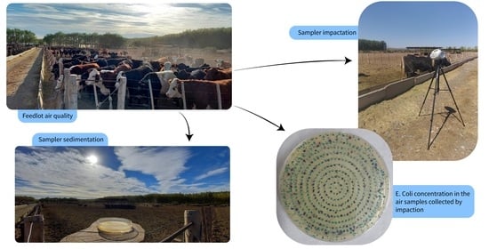
3.1. Sampling and Detection of Airborne E. coli Concentration

3.1.1. Sampling of Airborne E. coli

There are different methods for sampling bioaerosols, of which deposition and impaction belong to the relatively simple and most used collecting techniques [5,37] We included two types of sampling in our experiment: active and sedimentation samples. Airborne microorganisms were collected directly on Petri dishes prepared with a culture medium or nutrient [30,31,37]. Active measurements at LPR were made on 20 February 2020 and 5 April 2022 with an impaction microflow sampler (Microflow α Aquaria version 3.0.0 cod. G.1015) disposable 90 mm Petri dishes and a sampling speed of 30 L/min. The passive deposition samplings were all made on 5 April 2022. The impaction samplers were disinfected after each sampling with tissue paper soaked with 70% ethyl alcohol. The chromogenic culture media was CHROMagar™ (CHROMagar™ Orientation of CHROMagar).
Commonly, the concentrations of living microorganisms present in the air is the number of colony-forming units in the volume of air, the results of deposition sampling methods are expressed as bacterial colony-forming units (CFU) per unit area and unit time, so they cannot be compared directly with the results from volumetric measurements [5]. Samples were taken at a height of approximately 1.1 m and were georeferenced in situ, and the Petri dishes were distributed among the pens and windward and downwind from the emission points at the sites shown in Figure 1b (Mi). An additional measurement was made in the place where manure is stored (M23, not shown in Figure 1). The samples were kept cool until they arrived at the laboratory. Sampling times were set from 10 a.m. to 5 p.m. (LT, local time), which is when the greatest PM10 emissions take place, according to Bonifacio et al. [28].
The sampling method was designed during a prior experiment in a feedlot in Chel Cura (Choele Choel, Río Negro Argentina), where measurements were made with exposure times of 3, 5, and 10 min. Three-minute exposures within the pens resulted in saturated dishes, which hindered the measurement of CFU [38]. Based on these results, and considering that there were more cattle heads at LPR than in Chel Cura, as well as the studies by Bragoszewska et al. [30,39] and Environment Agency [40] the sampling speed was set at 30 L/min for active sampling (sites called Ai in Table 1). The locations of those sites are indicated as Mi in Figure 1b.
The sampling volume in the pens was 30 L and was augmented to 300 L with increasing distance from the more crowded areas. Deposition samples were called Pi (see Table 1) and were obtained from exposures of 10 and 30 min at the sites shown in Figure 1a (puntos Mi).

3.1.2. Microbial Analysis

The samples were incubated at 37 ± 1 °C for 48 h with readings at 24 h. Under the same conditions, a control measurement was made in CHROMagar medium using the reference strain E. coli ATCC 25922. The total count of bacteria present was also carried out, identifying them according to morphology, color and appearance.

3.2. Emission and Dispersion

USEPA [40] establishes a PM10 emission factor of 17 ton/1000 hd-yr as a methodology for the estimation of feedlot emissions. We estimated PM10 emissions based on these results adjusted by the number of heads in the pens to assess the emission; and Li et al. [37] we estimated bioaerosols as 25% of PM10 mass fraction.
The feedlot dispersion plumes were simulated using the HYSPLIT model, developed by the Air Resources Laboratory (ARL) [41], with meteorological observations from Neuquén station (see Figure 1a)—which is the closest one to the study area—and Global Data Assimilation System (GDAS) data. For modeling purposes, particles were assumed to be lifted by cattle activity and wind. The dry deposition rate was calculated assuming a particle density of 1.0 g·cm3 [12]. The values of the highest concentrations at the breathing level were estimated with a screening model.

4. Results and Discussion

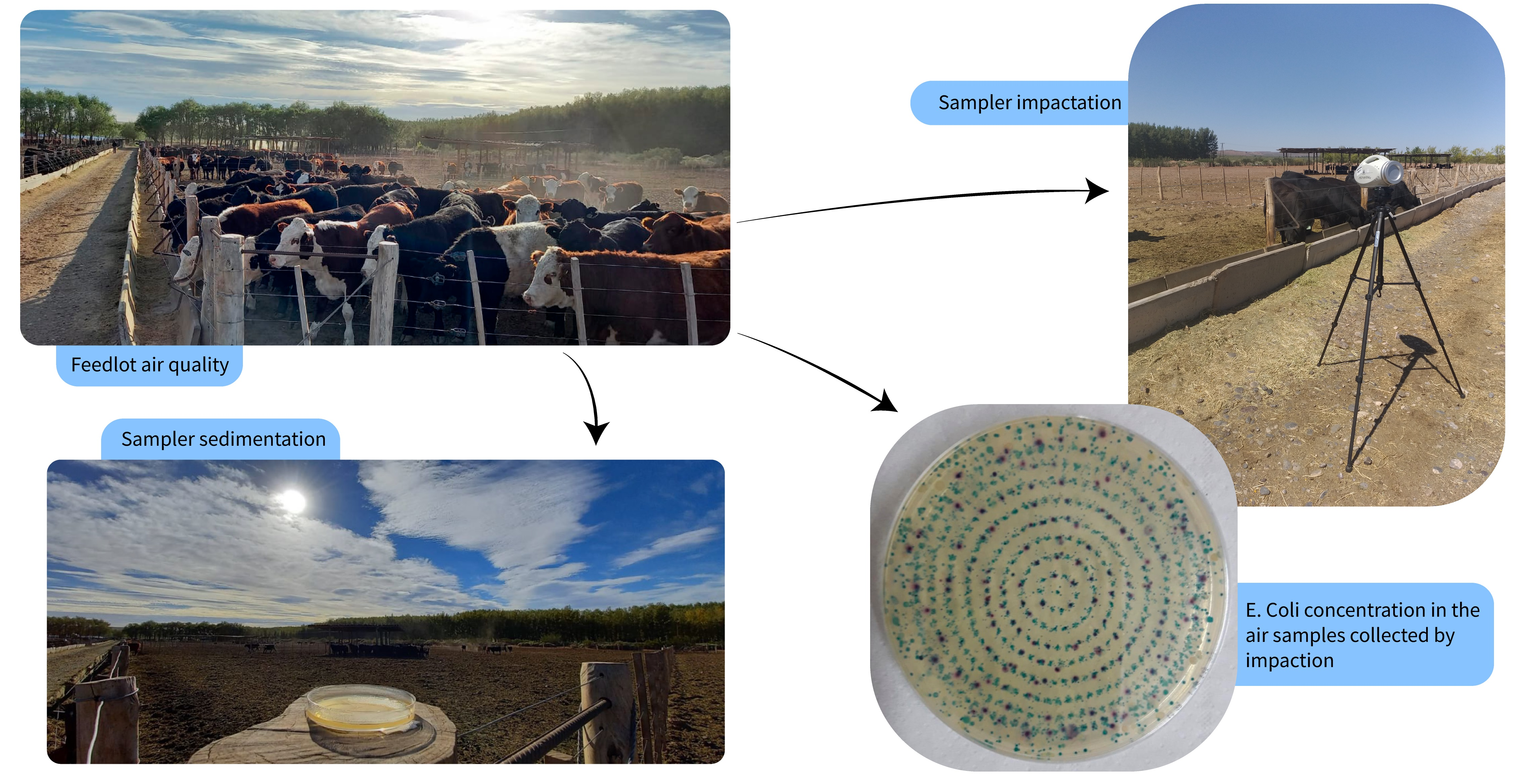
4.1. Weather Parameters and Airborne E. coli Concentration

The weather conditions during the sampling of 20 February 2020 and 5 April 2022 are informed in Table 2 and were estimated from GDAS data for the study area. The results of the active samplings in the field experiments showed that in-pen E-coli concentrations were greatest at sites M6 and M7 (see Table 3, Table 1). The maximum concentration of airborne E. coli in the two events under analysis was 2967 CFU/m3 and took place on 20 February 2020 (Table 3). On 5 April 2022, the maximum concentration was 33 CFU/m3. The average concentration was 1050 ± 1090 CFU/m3 on the 20 February 2020 and 8 ± 17 CFU/m3 on 5 April 2022 (Table 3), which amounts to a difference in concentration of 76.2%. According to the literature, concentration differences can be expected in connection to weather conditions and cattle activity [31].
The high temperatures that are prevalent in summer support the growth and physiological activity of bioaerosols [42]. The maximum growth rate of E. coli bacteria occurs in the range of 21–42 °C, and optimum growth is at 37 °C [43].The greatest count of E. coli was registered on 20 February 2020, after several days of air temperature ranging from 15.3 °C to 31.2 °C and an average ground temperature of 39.5 °C with low rainfall and low relative humidity. These ambient conditions favored dust and manure particle suspension by the light breeze (see Table 2). On 5 April 2022, the mean ground temperature was 30.3 °C at the time of sampling (see Table 2), and the air temperature range on the three previous days was 8.9–27.7 °C (see Table 2), with weak wind, which would limit bacteria growth and subsequent emission of particles from the surface into the air.
Factors affecting the abundance of microbial activity are quite complex and include meteorological parameters, weather conditions, the intensity of the source, and the geographical environment [30]. Zhong et al. [42] and Li et al. [31] analyzed the correlations between meteorological variables and bacteria concentration in bioaerosols and found that atmospheric temperature and wind speed have, respectively, positive and negative effects on bacterial concentrations; while relative humidity and wind direction would have no significant influence. The sampling results agree with those of Zhong et al. [42] who found that the seasonal distribution of bacterial concentration in bioaerosols was greatest in summer > autumn > winter > spring, with large fluctuations in summer and autumn.
To understand the airborne transport of E. coli, we collected air samples in situations and conditions that would allow describing the dissemination of these microorganisms around the source. In an exploratory analysis, we estimated the most unfavorable values associated with the highest concentrations at the breathing height, considering weather information and pen size (322 m × 176 m). The most unfavorable situations downwind of the feedlot would occur under a moderately stable atmosphere (SC (stability class): F), refs [36,44] at 183 m from the source, with the receptors assumed to be 1.5 m height above the ground (human breathing height). For which the following results were obtained:

4.2. Detection of E. coli by Impaction with Distance

E. coli concentrations in the air samples collected by impaction on 20 February 2020 were much higher than those obtained on 5 April 2022 (Table 3) in all comparable situations. At 180, 221, and 300 m from the feedlot pens, concentrations were 111 CFU/m3, 30 CFU/m3, and 20 CFU/m3, respectively. The presence of E. coli was observed to decrease by 82% with increasing distance from the source of the greatest emissions. Such a decrease agrees with the changes in concentration within the bioaerosol dispersion plume (see Table 4). The measurements at 180 m distance agree with the distance where the concentration peak would be found under worse air quality conditions using the screening method.
On 5 April 2022, the peak measured concentration was found at 160 m from the pen, with a value of 11 CFU/m3 (see Table 4) and a sampling period of 3 min.

4.3. Detection of E. coli by Deposition with Distance

The greatest deposition rate (DR) in the samples was 3.14 CFU/m2 s in the pen with the greatest number of animals (see Table 5). The second greatest value was 2.6 ± 0.5 CFU/m2 s, and in M1, M2, and M21 with a DR of 0.52 CFU/m2 s. The maximum DR in sites located far from the pens was 1.57 CFU/m2 s measured at M20, decreasing to 0.7 CFU/m2 s at M16 and to 0.52 CFU/m2 s at M21. The sampling point located 210 m away from the pens presented a deposition rate of 0.18 CFU/m2 s. In the area of manure collection (M23), the measure was 0.52 CFU/m2 s. (see Table 5 and Revised Supplementary Materials Tables S1–S5).

4.4. Detection of Total Bacteria with Distance on 5 April 2022

The active sampling total bacterial count on 5 April 2022 showed a greater presence of colonies inside the pens at M1 and M2 (see Table 6 and Figure 1). The maximum number of total bacteria colonies in air was 1467 CFU/m3, with a mean count of 889 ± 566 CFU/m3 on 5 April 2022 (see Table 6). Meanwhile, outside the pens, the mean bacteria count was 534 ± 586 CFU/m3, and the maximum was measured at M21 (see Table 6 and Figure 1), with 1378 CFU/m3 (see Table 6).
The passive sampling presented 51.35 CFU/m2 s inside the pens at M1 (see Table 7 and Figure 1) with a mean deposition of 26.45 ± 17.91 CFU/m2 s inside the pens (see Table 7) and a maximum of 60.78 CFU/m2 s at M20 (see Table 7 and Figure 1) downwind. The average deposition was 18.84 ± 17.94 CFU/m2 s (see Table 7).

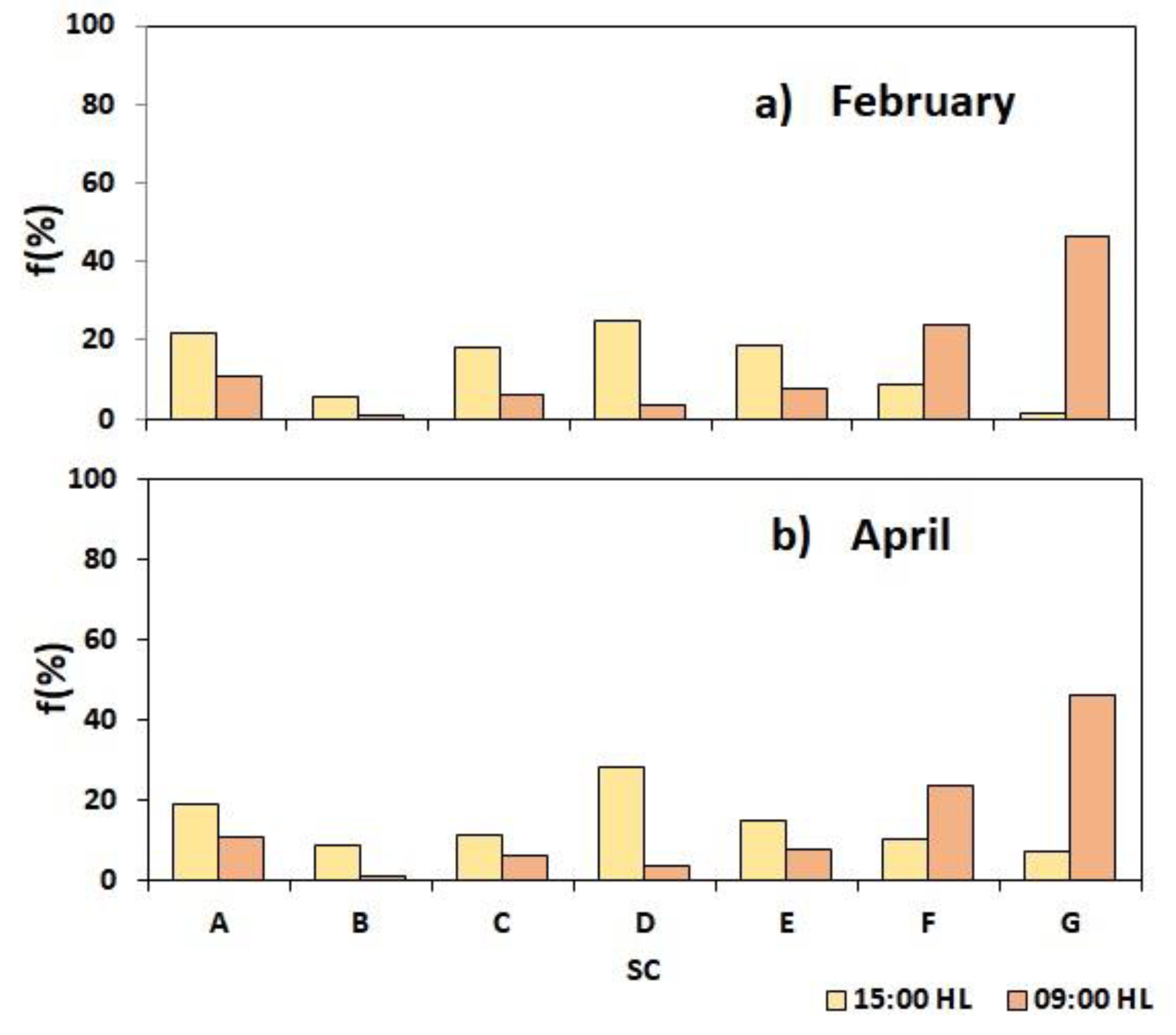
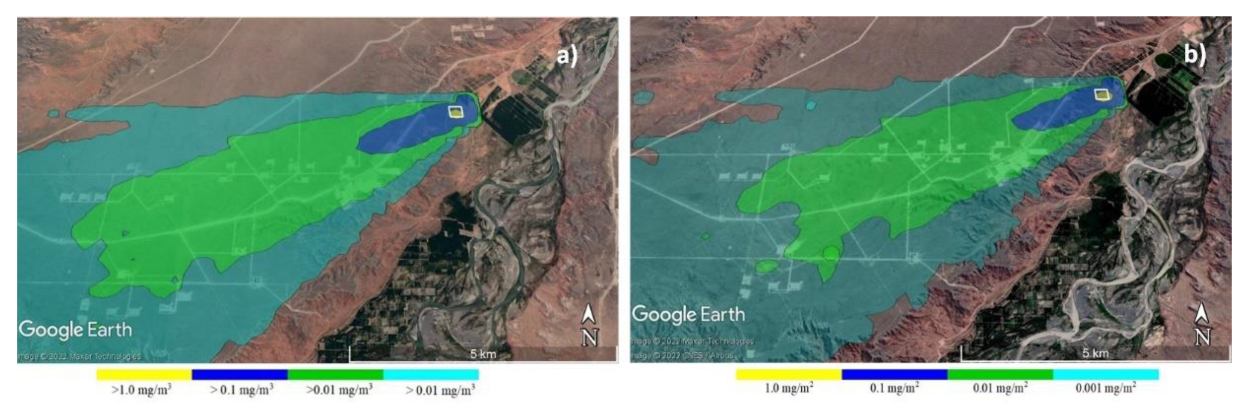
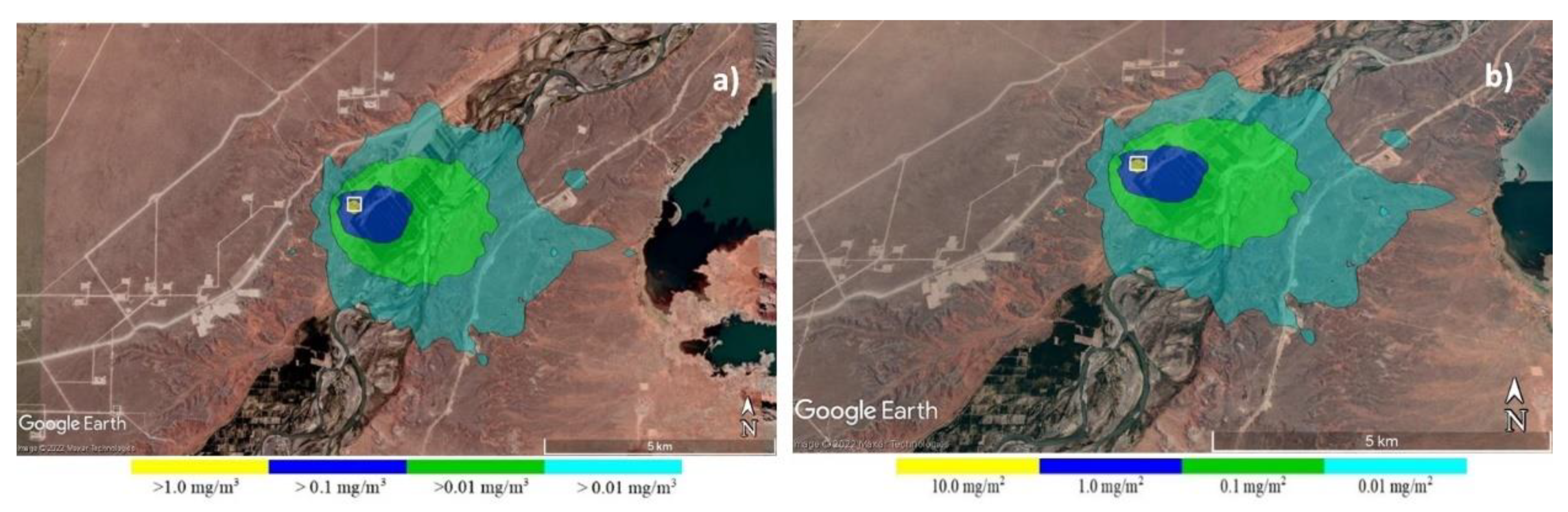
4.5. Bioaerosol Atmospheric Dispersion

Feedlot PM10 emissions were estimated based on the recommendations of USEPA [40], corrected by the number of heads at LPR, which resulted in a concentration of 27,945.2 kg/day 600 hd. Bioaerosols were estimated following the method defined in [44] and the result for LPR was 2812.5 mg/min [28] found that the emission from the feedlot pens they studied presented a diurnal variability with a peak between 10 am and 4 pm. Therefore, we assume that the emissions obtained in our work are associated with the time of maximum emissions at LPR.
Following the results of Jones and Harrison [7], we considered that bioaerosols were the 25% of the biological material that adhered to PM10, then, dispersion was modeled using the HYSPLIT model, and the 25% of the mean [40] pointed PM10 emission following the characteristics of LPR feedlot, resulting in 27,945.2 kg/day 600 hd. Dispersion estimates were calculated at the middle point of the sampling period.
Model vertical estimates show that the particles emitted on 5 April 2022 would reach a maximum height close to 1000 m, with peak concentrations in the lowest 500 m, while on 20 February 2020, the particles would reach 2000 m altitude with concentration peaks up to 1000 m. The maximum PM10 concentration on 20 February 2020 was 1.8 mg/m3, and 0.44 mg/m3 if only bioaerosol contribution is considered (see Figure 3a). The maximum concentration was at 340 m southwest of the feedlot, with a peak PM10 deposition of 8.6 mg/m2 and 2.1 mg/m2 of bioaerosols (see Figure 3b).
On 5 April 2022, the peak PM10 concentration was 7.3 mg/m3 or 1.7 mg/m3 if only bioaerosols are considered (see Figure 4a,b). The maximum deposition was 430 mg/m2 in the NE (M1–M4) and between 200 and 500 m downwind; bioaerosol concentration in a similar sector was 110 mg/m2 with a peak between 17 and 300 m from the center of the feedlot, in the farmer working area. These values agreed with the sampling results shown in Table 4. E coli concentration peaks on 20 February 2020 and 5 April 2022 were at 300 m and 210 m from the center of the feedlot. The spatial distribution of airborne bioaerosol concentrations obtained from the dispersion model agrees with the measured values (see Figure 3 and Figure 4 and Table 3). Site M6 had the greatest measured concentrations on 5 April 2022 and was located in the area of maximum concentration, as estimated by the model.

5. Conclusions

This paper presents the results of two sampling events of bacteria at 39 spots in La Paisana ranch, in Añelo (Neuquén, Argentina), with emphasis on E. coli, considering spots inside the pens, upwind and downwind of the feedlot, with different time steps, using a Microflow α equipment and deposition sampling methods.
Cattle are the major reservoir of STEC O157, a group of foodborne bacteria associated with severe human diseases, such as the UHS. The province of Neuquén has one of the highest UHS incidence rates in the world, which is connected to the high proportion of E. coli (clade 8 strain of STEC O157:H7) in Argentine cattle. In our field experiments, we did not evaluate the presence of that serotype in the air. This is an issue that needs to be studied with further measurements.
From the methodological point of view, the analysis indicates that sampling times of 1 min in the pens and 3 min downwind are correct to measure bacteria concentrations in this feedlot. E. coli bacteria were detected in both field experiments in the center of the pens and downwind areas. The passive method measures of total bacteria and the modeled dispersion estimates presented good agreement in terms of the spatial distribution of bioaerosol concentrations. The model proved to be an important tool in field experiments planning and distribution of downwind concentration; however, the spatial resolution should be higher.
Airborne aerosol concentrations are likely affected by weather conditions. The greatest concentration was found on 20 February 2020, which seemed to be associated with a higher surface temperature. The mean surface temperature on 20 February 2020 was 39.5 °C, which would stimulate the growth of E. coli as this temperature is within the range of maximum growth of these bacteria. The maximum PM10 concentration on 20 February 2020 was 1.8 mg/m3 and 0.44 mg/m3 if only bioaerosol contribution was considered with maximum heights up to 2000 m according to the height of the mixed layer. The 20 February 2020 maximum estimated deposition was at 340 m downwind. This would indicate that the greatest concentration of bacteria would be associated with summertime conditions, in agreement with Zhong et al. [42]. However, it should be noted that viable bacteria can be found at temperatures as low as 5 °C or less. The concentration of total bacteria on 5 April 2022 showed a similar pattern of E. coli distribution.
The air temperature range on the days preceding the measurements was favorable for the surface microbial load to persist. After that, cattle behavior and the wind would lift the bacteria into the air. Because the study area is located in an arid environment, the relative humidity in summer is particularly low. This situation would also favor the suspension of dust and manure particles from the ground by even a light breeze.
Bioaerosol emissions have a negative impact on the population, especially in areas with a high density of livestock and in the vicinity of intensive livestock operations. This is in line with the global trend toward the intensification and industrialization of animal breeding. The understanding of the spatial and temporal dynamics of atmospheric bioaerosols as well as the pathways of emission and transport is important for future research, mainly in areas such as the province of Neuquén, which has one of the highest HUS incidence rates in the world, connected to the high proportion of E. coli in Argentine cattle.

6. Note

The measurement experiment was planned according to the equipment and resources available. The results are indeed variable because measurements were carried out at different times and dates. In the first instance, we planned to measure under different meteorological situations and seasons to explore the general behavior of E.coli. In the planning stage of the research project, we had the possibility of full collaboration with the Central Laboratory of Neuquén province for the analysis, but the COVID-19 pandemic changed our plans. The laboratory was fully dedicated to covid PCR studies, and we also had trouble entering the feedlot. The costs of chemical analysis and field experiments increased, which impeded us from performing as many experiments as we had planned. We are considering performing more experiments in similar conditions to obtain more reliable results.

Supplementary Materials

The following supporting information can be downloaded at: https://www.mdpi.com/article/10.3390/atmos13111761/s1, Table S1. Concentration of bacteria E. coli in active sampling in LPR feedlot pens on 20th February 2020. Table S2. Concentration of E. coli in active sampling around LPR feedlot pens on 20th February 2020. Table S3. Concentration of E. coli in active sampling in LPR feedlot pens on 5th April 2022. Table S4. Deposition of bacteria E. coli in passive sampling in LPR feedlot pens on 5th April 2022. Table S5. Deposition of E. coli in the passive sampling around the LPR feedlot pens on 5th April 2022.

Author Contributions

Conceptualization, M.G.C. and P.A.P.; methodology, M.G.C., P.A.P. and L.A.P.; formal analysis, M.G.C., P.A.P. and L.A.P.; investigation, M.G.C., P.A.P., L.A.P., M.A.C. and P.N.M.; resources, P.A.P., L.A.P., M.A.C. and P.N.M.; writing—original draft preparation, M.G.C. and P.A.P.; writing—review and editing, M.G.C., P.A.P. and L.A.P.; supervision, M.G.C.; project administration, P.A.P.; funding acquisition, M.G.C. and P.A.P. All authors have read and agreed to the published version of the manuscript.

Funding

This research was funded by Río Negro National University (PI 40-A-715 UNRN).

Institutional Review Board Statement

Not applicable.

Informed Consent Statement

Not applicable.

Data Availability Statement

Not applicable.

Acknowledgments

We acknowledge Julieta Sepúlveda, Melina Tello Sandoval, Luciana Di Sario, and Priscilla Lopez Maldonado for the technical support and P. Richter for the English translation and text editing.

Conflicts of Interest

The authors declare no conflict of interest.

References

  1. Lighthart, B. The Ecology of Bacteria in the Alfresco Atmosphere. FEMS Microbiol. Ecol. 1997, 23, 263–274. [Google Scholar] [CrossRef]
  2. Matthias-Maser, S.; Bogs, B.; Jaenicke, R. The Size Distribution of Primary Biological Aerosol Particles in Cloud Water on the Mountain Kleiner Feldberg/Taunus (FRG). Atmos. Res. 2000, 54, 1–13. [Google Scholar] [CrossRef]
  3. Fröhlich-Nowoisky, J.; Kampf, C.J.; Weber, B.; Huffman, J.A.; Pöhlker, C.; Andreae, M.O.; Lang-Yona, N.; Burrows, S.M.; Gunthe, S.S.; Elbert, W.; et al. Bioaerosols in the Earth System: Climate, Health, and Ecosystem Interactions. Atmos. Res. 2016, 182, 346–376. [Google Scholar] [CrossRef] [Green Version]
  4. McGinn, S.M.; Chen, D.; Loh, Z.; Hill, J.; Beauchemin, K.A.; Denmead, O.T. Methane Emissions from Feedlot Cattle in Australia and Canada. Aust. J. Exp. Agric. 2008, 48, 183–185. [Google Scholar] [CrossRef]
  5. Clauß, M. Emission of Bioaerosols from Livestock Facilities: Methods and Results from Available Bioaerosol Investigations in and around Agricultural Livestock Farming; Johann Heinrich von Thünen-Institut: Braunschweig, Germany, 2020. [Google Scholar]
  6. McGinn, S.M.; Flesch, T.K.; Chen, D.; Crenna, B.; Denmead, O.T.; Naylor, T.; Rowell, D. Coarse Particulate Matter Emissions from Cattle Feedlots in Australia. J. Environ. Qual. 2010, 39, 791–798. [Google Scholar] [CrossRef]
  7. Jones, A.M.; Harrison, R.M. The Effects of Meteorological Factors on Atmospheric Bioaerosol Concentrations—A Review. Sci. Total Environ. 2004, 326, 151–180. [Google Scholar] [CrossRef]
  8. Clark, S.; Rylander, R.; Larsson, L. Airborne Bacteria, Endotoxin and Fungi in Dust in Poultry and Swine Confinement Buildings. Am. Ind. Hyg. Assoc. J. 1983, 44, 537–541. [Google Scholar] [CrossRef]
  9. Post, P.M.; Hogerwerf, L.; Bokkers, E.A.M.; Baumann, B.; Fischer, P.; Rutledge-Jonker, S.; Hilderink, H.; Hollander, A.; Hoogsteen, M.J.J.; Liebman, A.; et al. Effects of Dutch Livestock Production on Human Health and the Environment. Sci. Total Environ. 2020, 737, 139702. [Google Scholar] [CrossRef]
  10. Straumfors, A.; Heldal, K.K.; Eduard, W.; Wouters, I.M.; Ellingsen, D.G.; Skogstad, M. Cross-Shift Study of Exposure response Relationships between Bioaerosol Exposure and Respiratory Effects in the Norwegian Grain and Animal Feed Production Industry. Occup. Environ. Med. 2016, 73, 685–693. [Google Scholar] [CrossRef] [Green Version]
  11. Millner, P.D. Bioaerosols Associated with Animal Production Operations. Bioresour. Technol. 2009, 100, 5379–5385. [Google Scholar] [CrossRef]
  12. Jahne, M.A.; Rogers, S.W.; Holsen, T.M.; Grimberg, S.J.; Ramler, I.P. Emission and Dispersion of Bioaerosols from Dairy Manure Application Sites: Human Health Risk Assessment. Environ. Sci. Technol. 2015, 49, 9842–9849. [Google Scholar] [CrossRef] [PubMed]
  13. Kim, K.-Y.; Ko, H.-J.; Kim, D. Assessment of Airborne Microorganisms in a Swine Wastewater Treatment Plant. Environ. Eng. Res. 2012, 17, 211–216. [Google Scholar] [CrossRef]
  14. Douwes, J.; Wouters, I.; Dubbeld, H.; van Zwieten, L.; Steerenberg, P.; Doekes, G.; Heederik, D. Upper Airway Inflammation Assessed by Nasal Lavage in Compost Workers: A Relation with Bio-Aerosol Exposure. Am. J. Ind. Med. 2000, 37, 459–468. [Google Scholar] [CrossRef]
  15. Radon, K.; Schulze, A.; Ehrenstein, V.; van Strien, R.T.; Praml, G.; Nowak, D. Environmental Exposure to Confined Animal Feeding Operations and Respiratory Health of Neighboring Residents. Epidemiology 2007, 18, 300–308. [Google Scholar] [CrossRef]
  16. Sneeringer, S. Does Animal Feeding Operation Pollution Hurt Public Health? A National Longitudinal Study of Health Externalities Identified by Geographic Shifts in Livestock Production. Am. J. Agric. Econ. 2009, 91, 124–137. [Google Scholar] [CrossRef]
  17. Beran, G.W. Disease and Destiny–Mystery and Mastery. Prev. Vet. Med. 2008, 86, 198–207. [Google Scholar] [CrossRef] [PubMed]
  18. Klous, G.; Huss, A.; Heederik, D.J.J.; Coutinho, R.A. Human–Livestock Contacts and Their Relationship to Transmission of Zoonotic Pathogens, a Systematic Review of Literature. One Health 2016, 2, 65–76. [Google Scholar] [CrossRef] [Green Version]
  19. Rahman, S.; Mukhtar, S.; Wiederholt, R. Managing Odor Nuisance and Dust from Cattle Feedlots. 2008. Available online: https://www.semanticscholar.org/paper/Managing-Odor-Nuisance-and-Dust-from-Cattle-Rahman-Mukhtar/7e8ebd1f8c837fa7f4474ba509a9878b1b24a0f1 (accessed on 19 October 2022).
  20. Bush, J.; Heflin, K.; Marek, G.; Bryant, T.; Auvermann, B. Increasing Stocking Density Reduces Emissions of Fugitive Dust from Cattle Feedyards. Appl Eng Agric 2014, 30, 815–824. [Google Scholar] [CrossRef]
  21. Sweeten, J. Cattle Feedlot Manure and Wastewater Management Practices. In Animal Waste Utilization: Effective Use of Manure as a Soil Resource; Hatfield, J.L., Stewart, B.A., Eds.; CRC Press LLC: Boca Raton, FL, USA, 1998. [Google Scholar]
  22. Greig, J.D.; Ravel, A. Analysis of Foodborne Outbreak Data Reported Internationally for Source Attribution. Int. J. Food Microbiol. 2009, 130, 77–87. [Google Scholar] [CrossRef]
  23. Smith, J.L.; Fratamico, P.M.; Gunther, N.W. Shiga Toxin-Producing Escherichia coli. Adv. Appl. Microbiol. 2014, 86, 145–197. [Google Scholar] [CrossRef]
  24. Pianciola, L.; Chinen, I.; Mazzeo, M.; Miliwebsky, E.; González, G.; Müller, C.; Carbonari, C.; Navello, M.; Zitta, E.; Rivas, M. Genotypic Characterization of Escherichia coli O157:H7 Strains That Cause Diarrhea and Hemolytic Uremic Syndrome in Neuquén, Argentina. Int. J. Med. Microbiol. 2014, 304, 499–504. [Google Scholar] [CrossRef] [PubMed]
  25. Pianciola, L.; D’Astek, B.A.; Mazzeo, M.; Chinen, I.; Masana, M.; Rivas, M. Genetic Features of Human and Bovine Escherichia coli O157:H7 Strains Isolated in Argentina. Int. J. Med. Microbiol. 2016, 306, 123–130. [Google Scholar] [CrossRef] [PubMed]
  26. Berry, E.D.; Wells, J.E.; Bono, J.L.; Woodbury, B.L.; Kalchayanand, N.; Norman, K.N.; Suslow, T.V.; López-Velasco, G.; Millner, P.D. Effect of Proximity to a Cattle Feedlot on Escherichia coli O157:H7 Contamination of Leafy Greens and Evaluation of the Potential for Airborne Transmission. Appl. Environ. Microbiol. 2015, 81, 1101–1110. [Google Scholar] [CrossRef] [PubMed] [Green Version]
  27. Penner, J.E.; Andreae, M.O.; Annegarn, H.; Barrie, L.; Feichter, J.; Hegg, D.; Achuthan, J.; Leaitch, R.; Murphy, D.; Nganga, J.; et al. Aerosols: Their Direct and Indirect Effects, The Scientific Basis, Contribution of Working Group I to the Third Assessment Report of the Intergovernmental Panel on Climate Change; Dai, X., Maskell, K., Johnson, C.A., Eds.; Cambridge University Press: Cambridge, UK, 2001. [Google Scholar]
  28. Bonifacio, H.F.; Maghirang, R.G.; Auvermann, B.W.; Razote, E.B.; Murphy, J.P.; Harner, J.P. Particulate Matter Emission Rates from Beef Cattle Feedlots in Kansas—Reverse Dispersion Modeling. J. Air Waste Manag. Assoc. 2012, 62, 350–361. [Google Scholar] [CrossRef] [Green Version]
  29. Millner, P.; Suslow, T. CA Lettuce Research Board 2007-08: Concentration and Deposition of Viable E. coli in Airborne Particulates from Composting and Livestock Operations; National Agricultural Library: Salinas, CA, USA, 2008. [Google Scholar]
  30. Bragoszewska, E.; Mainka, A.; Pastuszka, J.S. Concentration and Size Distribution of Culturable Bacteria in Ambient Air during Spring and Winter in Gliwice: A Typical Urban Area. Atmosphere 2017, 8, 239. [Google Scholar] [CrossRef] [Green Version]
  31. Li, M.; Qi, J.; Zhang, H.; Huang, S.; Li, L.; Gao, D. Concentration and Size Distribution of Bioaerosols in an Outdoor Environment in the Qingdao Coastal Region. Sci. Total Environ. 2011, 409, 3812–3819. [Google Scholar] [CrossRef]
  32. Prohaska, M.C. Climates of Central and South America.; Swerdtfeger, W., Ed.; Elsevier Scientific Pub. Co.: Amsterdam, the Netherlands, 1976. [Google Scholar]
  33. Kottek, M.; Grieser, J.; Beck, C.; Rudolf, B.; Rubel, F. World Map of the Köppen-Geiger Climate Classification Updated. Meteorol. Z. 2006, 15, 259–263. [Google Scholar] [CrossRef]
  34. Lässig, J.L.; Cogliati, M.G.; Bastanski, M.A.; Palese, C. Wind Characteristics in Neuquen, North Patagonia, Argentina. J. Wind Eng. Ind. Aerodyn. 1999, 79, 183–199. [Google Scholar] [CrossRef]
  35. Gassmann, M.I.; Mazzeo, N.A. Air Pollution Potential: Regional Study in Argentina. Environ. Manag. 2000, 25, 375–382. [Google Scholar] [CrossRef]
  36. Pasquill, F. The Estimation of the Dispersion of Windborne Material. Meteorol. Mag. 1961, 90, 33–49. [Google Scholar]
  37. Li, Y.; Lu, R.; Li, W.; Xie, Z.; Song, Y. Concentrations and Size Distributions of Viable Bioaerosols under Various Weather Conditions in a Typical Semi-Arid City of Northwest China. J. Aerosol Sci. 2017, 106, 83–92. [Google Scholar] [CrossRef]
  38. Paez, P.A.; Cogliati, M.G.; Pianciola, L.A.; Mut, P.N.; Ciaramaría, E.; Caputo, M.; Tesán, I. Dispersion of PM10 Bioaerosols Associated with Intensive Cattle Breeding in Argentinian Patagonia Provinces. In Proceedings of the III Jornadas Internacionales y V Nacionales de Ambiente, Buenos Aires, Argentina, 12–14 May 2021; pp. 3–6. [Google Scholar]
  39. EPA. Screening Procedures for Estimating the Air Quality Impact of Stationary Sources, revised (Technical Report). 1992. Available online: https://www.osti.gov/biblio/6018929 (accessed on 19 October 2022).
  40. USEPA. Detecting and Mitigating the Environmental Impact of Fecal Pathogens Originating from Confined Animal Feeding Operations: Review; Bibliogov: Cincinnati, OH, USA, 2005.
  41. Stein, A.F.; Draxler, R.R.; Rolph, G.D.; Stunder, B.J.B.; Cohen, M.D.; Ngan, F. NOAA’s HYSPLIT Atmospheric Transport and Dispersion Modeling System. Bull. Am. Meteorol. Soc. 2015, 96, 2059–2077. [Google Scholar] [CrossRef]
  42. Zhong, X.; Qi, J.; Li, H.; Dong, L.; Gao, D. Seasonal Distribution of Microbial Activity in Bioaerosols in the Outdoor Environment of the Qingdao Coastal Region. Atmos. Environ. 2016, 140, 506–513. [Google Scholar] [CrossRef]
  43. Ingraham, A.G.; Marr, J.L. Escherichia coli and Salmonella: Cellular and Molecular Biology, 2nd ed.; Microbiology, A.S., Ed.; American Society for Microbiology: Washington, DC, USA, 1996. [Google Scholar]
  44. Alghamdi, M.A.; Shamy, M.; Redal, M.A.; Khoder, M.; Awad, A.H.; Elserougy, S. Microorganisms Associated Particulate Matter: A Preliminary Study. Sci. Total Environ. 2014, 479–480, 109–116. [Google Scholar] [CrossRef]
Figure 1. (a) Location of La Paisana ranch (LPR) in Neuquén. (b) Enlarged satellite image of the pens at LPR (yellow lines) and location of the sampling points (Mi) described in Table 1.
Atmosphere 13 01761 g001
Figure 2. Relative frequency (f [%]) of atmospheric stability (SC, [36]) in Neuquén as a function of the month ((a) February, (b) April) at 09:00 LT (light yellow) and at 15:00 LT (dark yellow), for the period 2015–2021. Classes: A: extremely unstable; B: moderately unstable; C: lightly unstable; D: neutral; E: lightly stable; F: moderately stable, G: extremely stable. Data from the Real-time Environmental Applications and Display sYstem (READY, http://www.ready.noaa.gov (accessed on 10 May 2022)).
Atmosphere 13 01761 g002
Figure 3. (a) Bioaerosol concentration downwind from the feedlot from HYSPLIT on 20 February 2020 at 13:00 UTC considering an emission source located from 0 to 1.5 m above the ground (b) deposition from HYSPLIT 20 February 2020 at 14:00 UTC.
Atmosphere 13 01761 g003
Figure 4. (a) Bioaerosol concentration downwind of the feedlot from HYSPLIT on the 5 April 2022 at 13:00 UTC considering an emission source between 0 and 1.5 m above the ground (b) deposition from HYSPLIT for the 5 April 2022 at 14:00 UTC.
Atmosphere 13 01761 g004
Table 1. Correspondence between sampling points (Mi) and passive (Pi) and active (Ai) measurements of the samplings of days 20 February 2020 and 5 April 2022.
Mi20 February 20205 April 2022
AiPiAi
M1A2P11–P12A14
M2A1P9–P10A15
M3A3
M4A4
M5A5P7–P8A16–A17
M6A6
M7 P1–P2A18
M8A7
M9A8
M10A9
M11 P5–P6A19
M12A10
M13A11
M14A12
M15A13
M16 A20
M17 P17–P18
M18 P19
M19 P20
M20 P15–P16A21
M21 P13–P14A22
M22 A24
M23 A25 (manure storage)
Table 2. Mean meteorological parameters during the field experiments at LPR (15 UTC to 18 UTC). Rainfall (PP, mm), relative humidity (RH, %), evolution of atmospheric stability (SC, [36], wind speed (v, m/s), wind direction (DD), mean air temperature (T, °C), height of the mixed layer (H, m), atmospheric pressure (P, hPa), downward shortwave radiation range (I, W/m2), temperature range on the 3 days prior to the sampling (RT, °C), 3-hourly soil moisture during the sampling period (RTS, °C) (source: NOAA Air Resources Laboratory). Rainfall corresponds to days 17 February 2020 and 3 April 2022.
20 February 20205 April 2022
DDENE–ESW–NE
V (m/s)2.6–3.9
3.9–6.7
<0.5
3.3
SCE–D–CE–E–D
PP (mm)0.5
(17 February 2020)
2.1
(3 April 2022)
T(°C)21.821.2
RH (%)20.023.6
P (hPa)10211011
H (m)<2069.8<1470
I (W/m2)523–605397.7–450
RT (°C)15.3–31.28.9–27.7
TSm (°C)39.530.3
Table 3. Average E. coli concentration per m3 of air (Cm, CFU/m3), concentration standard deviation (STC), minimum concentration E. coli per m3 of air (Cmin, CFU/m3), maximum concentration per m3 of air (Cmax, CFU/m3), number of samples (N) within the LPR pens. Sampling dates: 20 February 2020 and 5 April 2022. w/c: Petri dishes without count.
20 February 20205 April 2022
Cm (CFU/m3)10508
STC109017
Cmin (CFU/m3)w/cw/c
Cmax (CFU/m3)296733
N55
Table 4. E. coli concentration per m3 of air (R, CFU/m3), sampling site (ID), wind direction (DD), wind speed (v, m/s), distance between the sampling site and the pen with the highest E. coli concentration (M6 on 20 February 2020 and M7 on 5 April 2022) (D, m), sampling duration at 30 L/min (T, min), sampling time (hh:mm, local time (LT) of samplings on 20 February 2020 and 5 April 2022. w/c: Petri dishes without count.
Datehh:mm
(LT)
IDDDv
(m/s)
D
(M6, M7–Mi)
(m)
T
(min)
R
(CFU/m3)
20 February 202013:26M8 (A7)E2.0–3.6 72167
13:45M10 (A9)E3.6–<5.61823111
13:55M12 (A10)NE3.6–<5.6 221333
14:15M14 (A12)NE2.0–3.6 300520
5 April 202213:03M20 (A21)SSE<0.5 160311
13:15M21 (A22)SSE<0.5 553w/c
13:45M16 (A23)NE<0.5 1743w/c
14:08M22 (A24)NE<0.521010w/c
Table 5. Total mean E. coli deposition rate (DRm, CFU/m2 s) standard deviation (ST), minimum E. coli deposition rate (DRmin, CFU/m2 s), maximum E. coli deposition rate (DRmax, CFU/m2 s), number of samples (N). Sampling date: 5 April 2022, sampling site: withing the pens (INT), around the pens (OUT). w/c: saturated Petri dishes without count.
INTOUT
DRm (CFU/m2 s)1.350.43
ST1.240.50
DRmin (CFU/m2 s)w/cw/c
DRmax (CFU/m2 s)3.141.57
N79
Table 6. Average concentration of total bacteria per m3 of air (Cm, CFU/m3), concentration standard deviation (STC), minimum concentration of total bacteria (Cmin, CFU/m3), maximum concentration (Cmax, CFU/m3), number of considered samples (N). Sampling date: 5 April 2022, sampling site: within the pens (INT), around the pens (OUT).
INTOUT
Cm (CFU/m3)889534
STC566586
Cmin (CFU/m3)26723
Cmax (CFU/m3)14671378
N55
Table 7. Mean total bacteria deposition rate (DRm, CFU/m2 s) standard deviation (ST), minimum total bacteria deposition rate (DRmin, CFU/m2 s), maximum total bacteria deposition rate (DRmax, CFU/m2 s), number of samples (N). Sampling date: 5 April 2022, sampling site: within the pens (INT), downwind the pens (OUT).
INTOUT
DRm (CFU/m2 s)26.4518.84
ST17.9117.94
DRmin (CFU/m2 s)9.962.1 6
DRmax (CFU/m2 s)51.3560.78
N79
Publisher’s Note: MDPI stays neutral with regard to jurisdictional claims in published maps and institutional affiliations.

