Article

Effects of Local Vegetation and Regional Controls in Near-Surface Air Temperature for Southeastern Brazil

by
Rafael Cesario de Abreu
*,
Ricardo Hallak
and
Humberto Ribeiro da Rocha
Instituto de Astronomia, Geofísica e Ciências Atmosféricas (IAG-USP), São Paulo 05508-090, Brazil
*
Author to whom correspondence should be addressed.
Atmosphere 2022, 13(11), 1758; https://doi.org/10.3390/atmos13111758
Submission received: 30 July 2022 / Revised: 24 August 2022 / Accepted: 27 August 2022 / Published: 26 October 2022
(This article belongs to the Special Issue Urban Heat Islands and Global Warming)

Abstract

:
The spatial range of near-surface air temperature average and trends for Southeast Brazil in recent decades motivated us to investigate the causality of local vegetation and other geophysical controls at the regional scale to explain the spatial variability of the average maximum and minimum temperature (Tmax and Tmin). We used measurements from 52 weather stations between 1985 and 2010. Using linear regression, NDVI and cloud cover were significant to explain spatial variability of Tmax and Tmin. With the Generalized Additive Model (GAM), we improved temperature-dependent relationships with regional geophysical controls, and local scale NDVI. The modeling of Tmax and Tmin showed non-linear and combined relationships with geographical position (lat,lon) jointly expressing the effects of zonality and continentality, and NDVI at distances of 300 m and 3000 m. For Tmin, geographical position and altitude responded with an amplitude of ≃5 °C each, and NDVI with ≃3 °C. Similarly, the geographical position and altitude were significant for Tmax, with an amplitude of ≃5 °C each, and cloud cover with ≃3.5 °C. Our findings help to clarify the local scale controls of near-surface air temperature and stress the need to increase resilience against adversities of global climate change and increasing urbanization, by providing metrics to predict the effects of nature-based solutions within the urban space.

1. Introduction

The average global near-surface air temperature increased 0.85 °C [0.69 °C to 0.95 °C] between 1995–2014 relative to 1850–1900, dominated by increasing anthropogenic greenhouse gases and a minor contribution from aerosols and other natural sources that range from months to decades as solar radiation, volcanism, sea salt, and mineral dust [1]. However, this warming rate showed a large spatial variability across continental areas due to other anthropogenic factors like land cover change, increasing urbanization, and aerosols from industrial processes that contribute to either warming or cooling at the regional scale [2]. For Southeastern Brazil (SEB), a large and populated region larger than 900,000 km2, with more than 89 million inhabitants, [3] reported warming of 1.1 °C in 50 years (1955 to 2004) using CRUTEM4 data [4], well above the global average, but also attributed mostly to greenhouse gases and in agreement with the global scale effect [5]. However, at SEB there is a lack of information about the spatial variability of temperature trends, and only local studies are available [6,7]. We suspected even more about the spatial variability by analyzing historical trends from 52 weather stations in SEB. They showed a mean of 0.25 °C 10 yr 1 across stations for daily averaged temperature, which compared well with the regional mean of de Abreu et al. [3], but with a high range of values showing both cooling and warming trends, of +0.02 to +0.51 °C 10 yr 1 for minimum daily temperature (Figure 1a), from −0.01 to +0.46 °C 10 yr 1 for average temperature (Figure 1b), and from −0.1 to +0.60 °C 10 yr 1 for maximum daily temperature (Figure 1c).
The pattern with a pronounced spatial heterogeneity in temporal temperature trends (Figure 1) motivated us to investigate in depth the spatial controls of the long-term mean temperature. Various authors reported connections between the temporal trends and the controls affecting the mean near air-surface temperature, for example, the land cover [8,9,10] and topography [11,12], that can possibly enhance or diminish how the large-scale controls affect the local response of temporal changes. Therefore, to identify the likely controls of local-regional variability in temporal trends, we have first to guarantee the physical consistency of the measurements, and then obtain the controls of variability in the mean state of temperature.
The SEB contributes over 50% of the national Gross Domestic Product (GDP) with services, agricultural and industrial goods, as well as headwaters for hydroelectricity and human water supply, where the impacts of climate change are risky due to significant exposure and vulnerability [13,14,15]. The region is spatially complex in topography and land cover, where latitudinal variation explains up to 50% of average temperature range, and longitude, which is a proxy for continentality, has a lower impact [16]. Rodriguez-Lado et al. [17] used a linear regression model to study the patterns of spatial variability in the state of São Paulo, which is part of the SEB, with altitude and latitude as independent variables, with no significant impact on longitude. The influence of continentality is confounded with the effects of two large mountain ranges placed parallel to the coastline (Serra do Mar and Serra da Mantiqueira), wherein a combined effect of sea breeze and orographic circulation both contribute to cloud cover and cold air advection [18]. In SEB the land cover in rural areas is dominated by pastureland and sugarcane plantations, and an increasing urbanization that enhances local warming [19]. For example, the urban heat island effect in the city of São Paulo was characterized by accelerated expansion of urban areas since the early 20th century, and is partly responsible for increasing local air temperature [20]. However, the urban heating is not homogeneous over it spatial extent and depends on many different physical factors such as diurnal cycle, atmospheric turbulence, thermal properties of constructed materials, and urban morphology as well as the background temperature [8,21,22]. On this subject, Kagawa-Viviani and Giambelluca [12] used multiple linear regression at the regional scale in Hawaii and showed a dependency of the spatial distribution of minimum temperature with vegetation and wind speed, which was not observed for maximum temperature, that had a dependency with precipitation and cloud cover. Also, other features might explain the effects at the local scale with complex topography, like slope and aspect [23].
In general, the studies of attribution of spatial variability of temperature in SEB are modest, using a limited set of independent variables that did not include likely effects of land cover and cloud cover caused by mesoscale circulation [16,17]. To contribute to this understanding, multiple linear regression (MLR) is advantageous, as a simple and parsimonious model for explicit quantification of different independent variables. However, MLR has intrinsic restrictions, like assuming a linear relationship between the dependent and independent variables. The Generalized Additive Model (GAM) was developed to overcome this limitation, as a generalization of the Generalized Linear Model (GLM). GAM fits smoothing functions to build relationships between a set of predictors and the predicted variable instead of assuming a linear dependency [24]. Still, relationships in GAM can be easily interpreted graphically for each independent variable, and provide inferences about individual contributions, differently from more complex non-linear methods like neural networks and other “black box” types of models.
Our objective is to assess the influence of local vegetation and regional scale geophysical controls on the spatial variability of near-surface temperature in Southeastern Brazil. Using a wide network of weather stations, and with the attempt to understand and describe a simple way of showing the dependencies of temperature with the geophysical features of zonality and continentality, altitude, cloud cover, and as a novelty the influence of local vegetation, we used parsimonious linear (MLR) and non-linear (GAM) models.

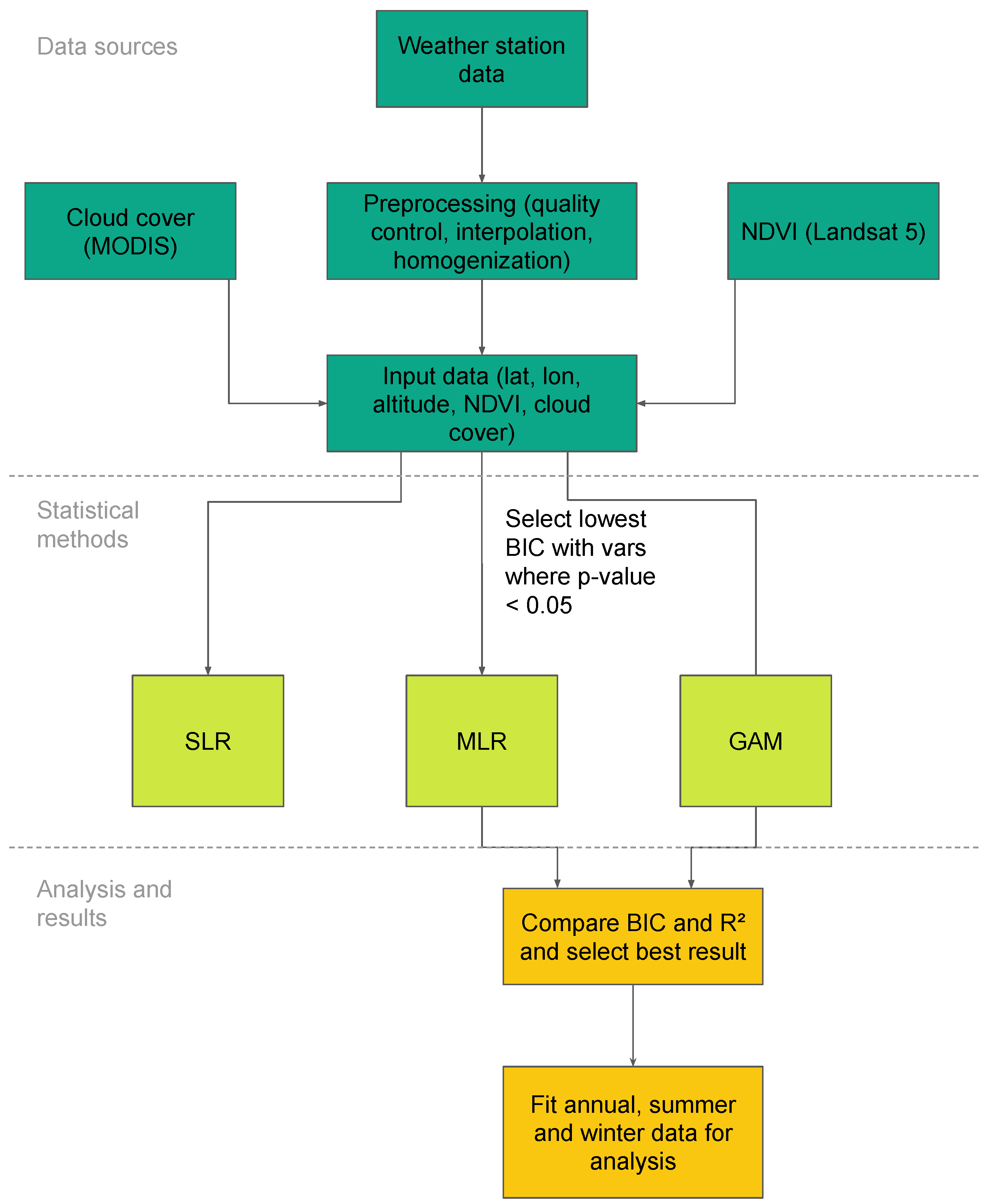
2. Materials And Methods

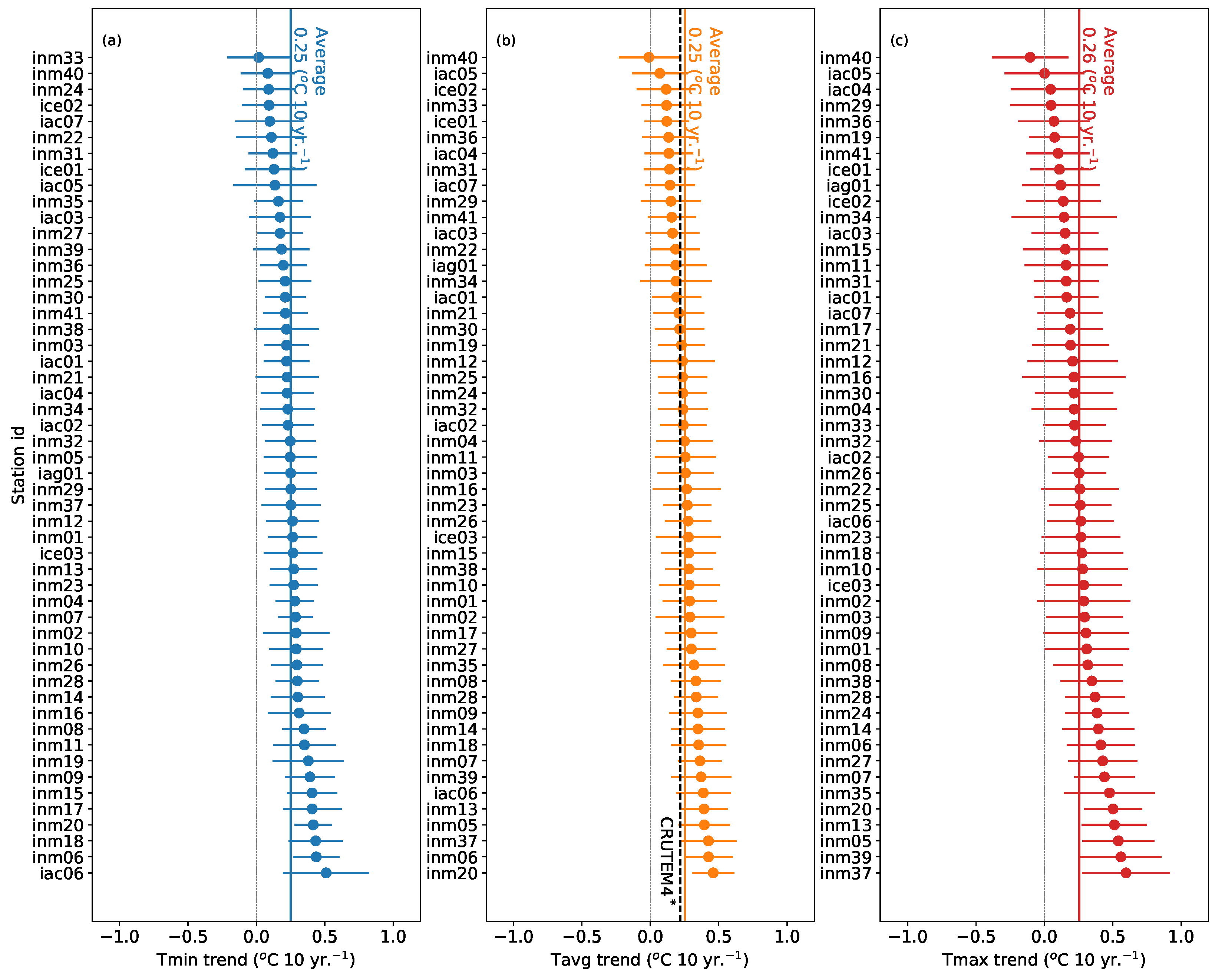
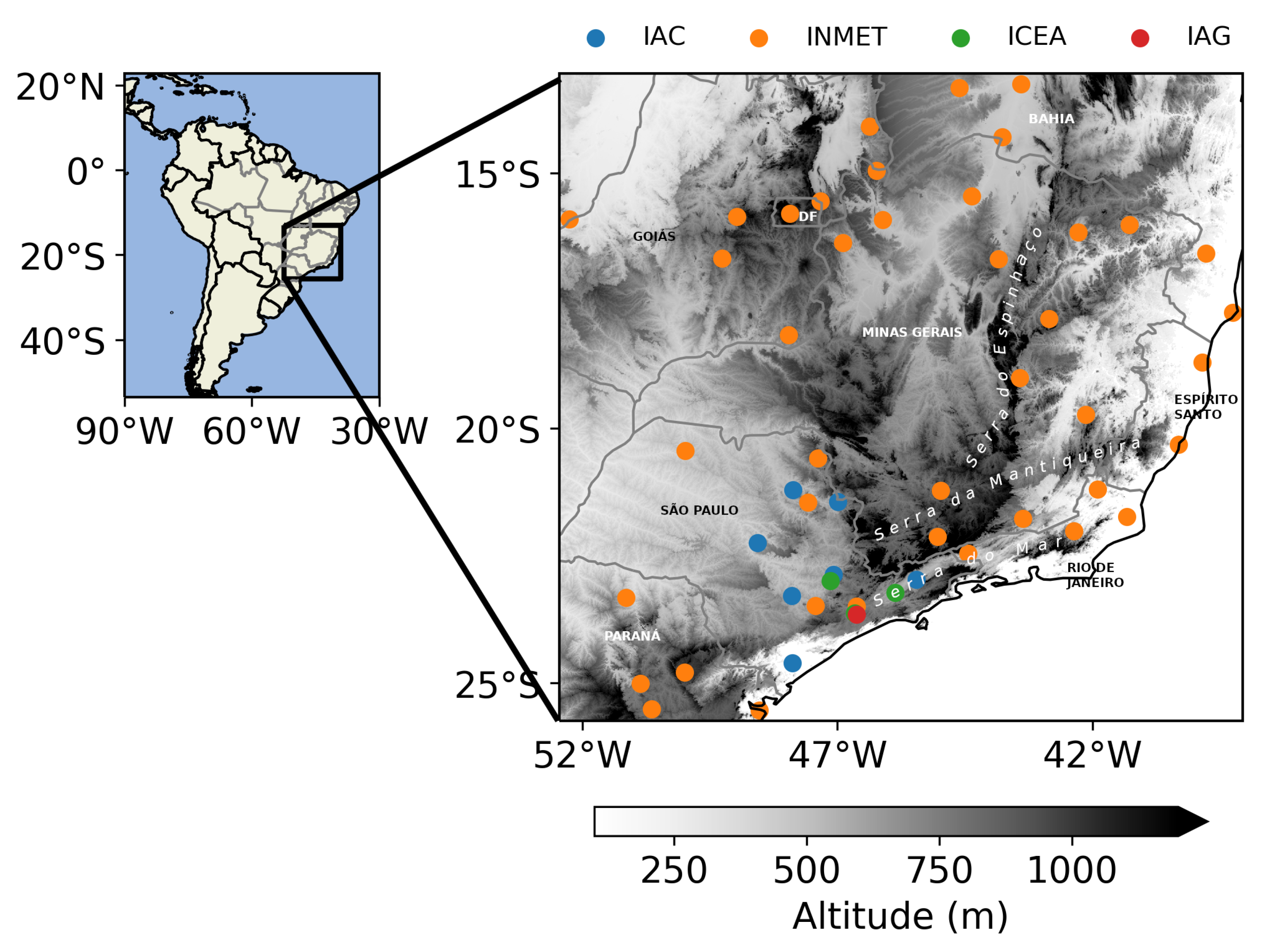
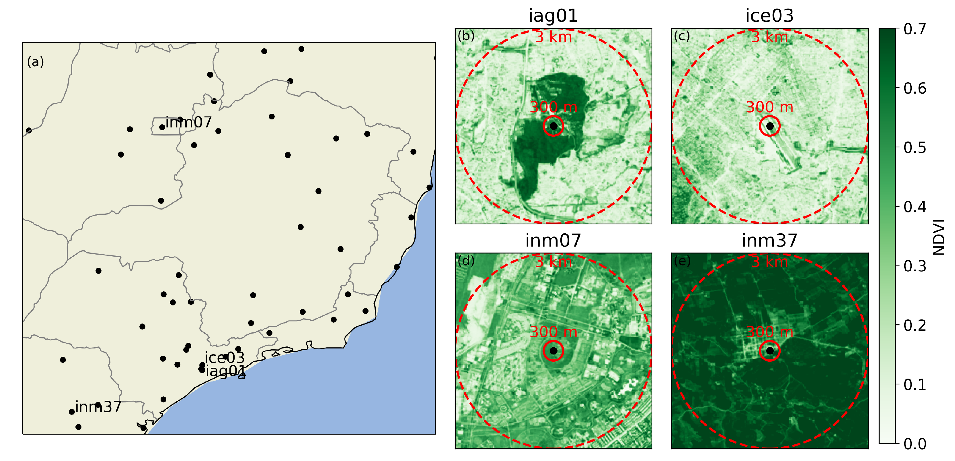
2.1. Weather Station Information

We used minimum and maximum air temperature data (Tmin, and Tmax, respectively) from a network of weather stations in Southeast Brazil (INMET, IAC, ICEA, and IAG institutes) (Figure 2). We only used conventional weather stations that are installed according to standards about site selection and exposure, and used the longest available period to compute the climate means [25,26]. We selected the years from 1985 to 2010, which was optimum because of satellite data availability to calculate the Normalized Difference Vegetation Index (NDVI) values and by maximizing the number of available stations from IAC network, which was available until 2010. We quality controlled the available data by first checking metadata for the exact location of each station to calculate NDVI and fill in missing information about altitude. The second step included comparing the timeseries with predefined thresholds of physically plausible values, persistency of repeated values, and discarding data outside the boundaries defined by three times the standard deviation. We also compared it with nearby stations when more than six of them were available in a 100 km radius of the target stations, according to Meek and Hatfield [27] and Shafer et al. [28]. Weather stations that were moved during the selected period were not used in the analysis, resulting in 52 stations that met all requirements (Table S1). A total of 15 stations have between 10–30% of missing data for Tmin and 20 for Tmax, and only five have between 20–30% for both Tmin and Tmax.
We interpolated missing data with Empirical Orthogonal Functions (EOF) according to the method described in Beckers and Rixen [29], which is better suited to interpolate larger periods of missing data [30]. According to this method, we start with the average of each station as a first guess for the missing data. Singular Value Decomposition (SVD) is then applied to the data matrix X ( n × s dimensions, where n = the number of days, s = number of stations). We retain m components to reconstruct the original matrix and create a new estimate of the original matrix. The new estimates are then replaced at the missing points in matrix X , and the process is repeated iteratively until convergence. To calculate the optimum number m of components to be used, 2% of missing data is randomly added to the original matrix and used to calculate the root mean squared error (RMSE). We select the number m with the lowest RMSE for the interpolation. This study used m = 5, which had an RMSE of 1.4 °C for minimum temperature. As a comparison, using inverse distance weighting (IDW) resulted in an RMSE of 2.1 °C. After the interpolation of missing values, we homogenized the data (described in Section S2), which is important to reduce the influence of random errors, detected through breakpoints in the timeseries, and caused by changes in instruments, drift, transcribing errors, that are not available in the metadata. We kept, however, stations where changes in NDVI and land use possibly occurred.
We used NDVI estimated by Landsat 5 satellite data (with 30 m of spatial resolution), using all available images for each of the 26 years of data. Then, the temporal average was calculated (Figure S3). We computed the spatial average using a circle with a variable radius with the origin at the station coordinates. After a sensitivity analysis with the length of the radius, we selected 300 m for the consolidated averages, based on the highest correlation with Tmin in the annual aggregation (Figure S4a). Altitude was selected from metadata when available, and we used the estimates from Shuttle Radar Topography Mission (SRTM [31]) when not. Cloud cover was estimated from a 15-year average (2000–2014) from the MODIS satellite with 1 km of spatial resolution [32].

2.2. Statistical Model

We used two models to represent the spatial variability of air temperature: Multiple Linear Regression and Generalized Additive Model, which can be expressed as the sum of smoothing functions f j [33]:
Y = α + j = 1 p f j ( X j ) + ϵ
where Y is the dependent variable (Tmin, Tmax), α is the intercept term, X j is the jth independent variable (j = 1, …, p; p = number of regressors), and ϵ is the residual error which has a normal distribution with zero mean and constant variance. The smoothing functions in Equation (1) have the ability to fit non-linear relations between the independent and dependent variables, however they are fitted following a penalized least squares algorithm to penalize too wiggly functions preventing an overfit of the model. The Generalized Cross Validation (GCV) is used to estimate the penalization for each variable [24]. By doing so, if the penalization is large we can even fit linear relations between the predictor and predicted variable. We used the concept of estimated degrees of freedom (edf) to determine whether or not the relations are linear since if edf ≥ 2, there is strong evidence that a nonlinear function might be the best fit [24]. We used the following source equation to fit the GAM:
T ^ = α ^ + f ^ 1 ( altitude ) + f ^ 2 ( NDVI ) + f ^ 3 ( cloud cover ) + f ^ 4 ( lon , lat )
Every function f ^ is fitted using the mgcv package for R [24], and the estimator α ^ is the spatial sample mean of the dependent variable T. The model was fitted individually for each of the following time aggregations: summer (December, January, and February), winter (June, July, and August), and annual (January to December). We highlight the usage of a single term for representing the zonal and continental effects through f 4 (lon,lat) that will be discussed in more detail in the results.
GAM is based on smoothing functions that require many different parameters to represent non-linear dependencies and therefore have a greater degree of complexity when compared with MLR. In the case of MLR, the model that we used is analogous to Equation (2), where f j ( X j ) = β j X j and, therefore:
T ^ = α ^ + β ^ 1 altitude + β ^ 2 NDVI + β ^ 3 cloud cover + β ^ 4 lon + β ^ 5 lat
Equation (3) has a maximum of six degrees of freedom, one for each regressor, while a GAM model can have more estimated degrees of freedom, depending on the nonlinearities found in the data. Therefore we compare the results for Equations (2) and (3) with the same regressors.
The models were evaluated according to the Bayesian Information Criteria (BIC), BIC = n SSE n log n + p log n , where SSE is the sum of squared residuals and n is the number of data samples. The lower the BIC, the lower the error; however, a penalization term accounts for the number of parameters in the model, prioritizing more parsimonious models with fewer parameters. To ensure that we are using the most conservative model, we tested all possible combinations of terms from Equations (2) and (3) (15 possibilities for GAM and 31 for MLR) and selected the model in which all terms were statistically significant with a 5% significance level and with the lowest BIC. A flow chart of the main steps is presented in Figure 3.
To detect if collinearity effects would be a problem in the model, affecting the interpretation of the results, we calculate the variance inflation factor (VIF), which estimates how much of the variance of the parameters in the regression is inflated in comparison with the case where they are linearly independent. The maximum value of VIF was 1.64 for latitude, which is inside the range of recommended values and should not cause any significant problems due to the collinearity of the regressors [34].

3. Results and Discussion
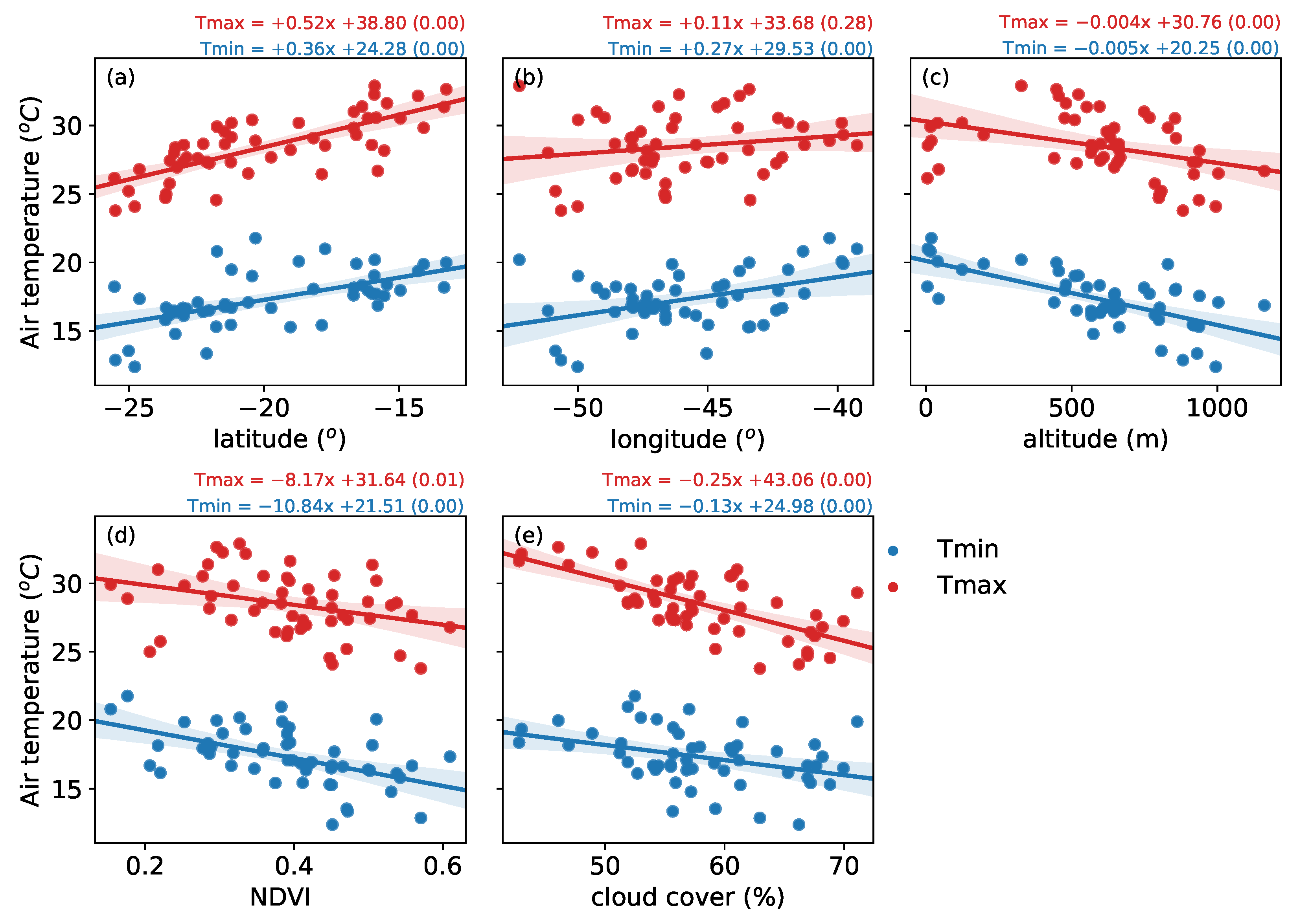
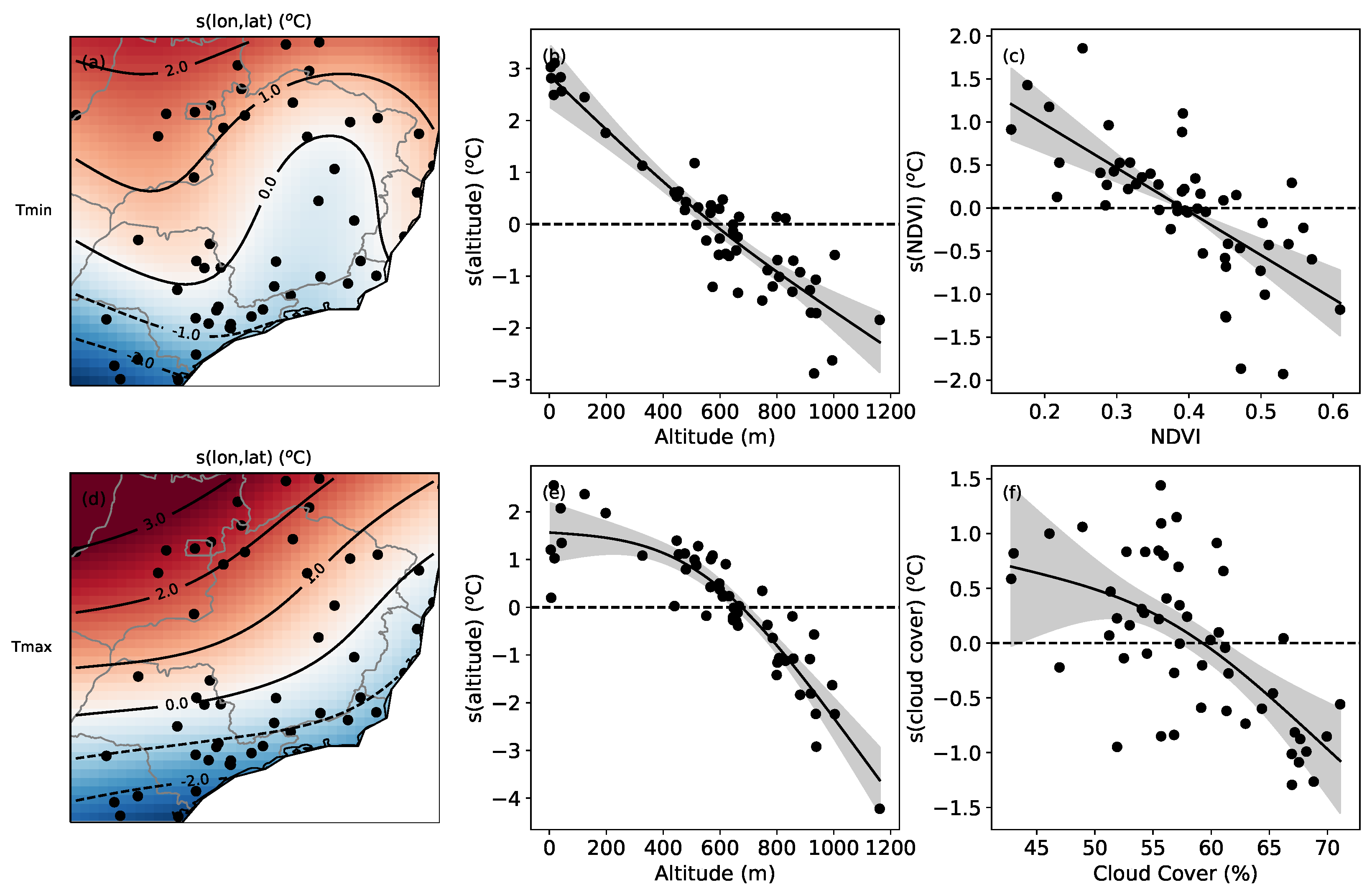
To elucidate the possible dependency of the average temperature with the selected regressors (latitude, longitude, NDVI, and cloud cover), we show the scatter plot for the annual average Tmax and Tmin (Figure 4) with each independent variable for a visual inspection of the relationship between them. We notice a wide range of average temperatures of almost 10 °C, to be more precise, between 12.4 and 21.8 °C (17.3 ± 2.0 °C) for Tmin and between 23.8 and 32.9 °C (28.5 ± 2.3 °C) for Tmax. We fitted the simple linear regression (SLR), and all scaling factors are statistically significant (p-value < 5%), except for Tmax and longitude (p-value = 0.19), suggesting that there is a dependency between each pair of variables. Based solely on the scaling factor, Tmax has a greater sensitivity than Tmin with latitude and cloud cover, while Tmin is more sensitive to NDVI, longitude, and altitude. In particular, we notice an atypical pattern between Tmax and altitude, with a heterogeneous distribution of points close to altitudes of zero meters.

3.1. Model Fitting

The estimated model parameters for MLR ( β ^ j ) and GAM (edf) are available in Table 1, with the respective R2 and BIC for the fitted model. They show that both models have a high percentage of the explained variance for temperature, with R2 between 86% and 94%. GAM explains a higher percentage than MLR, with a difference of almost 9% for Tmax and 7% for Tmin, and a lower BIC. For Tmax, MLR had five degrees of freedom (number of statistically significant independent variables), while for GAM there were 8.9 edfs (sum of the individual edfs for each independent variable). For Tmin MLR showed four degrees of freedom, while GAM had 10.3 edfs.
We noticed that the fitted functions using GAM are significant for Tmax with (lon,lat), altitude, and cloud cover, and Tmin with (lon,lat), altitude, and NDVI. For MLR, the fitted linear functions were the same as GAM, except for longitude, which was not statistically significant for Tmin. The fitted function for NDVI using GAM has an edf close to 1, which suggests a linear relation with Tmin, with no significant gain compared to MLR. Still, for Tmin, the relationship with altitude was slightly non-linear (edf = 1.55). For Tmax, the edf of altitude and cloud cover is close to 2, suggesting a non-linear relationship. For both Tmin and Tmax, the function s(lon,lat) was the one with the highest edf, 7.71 and 5.40, respectively. The MLR fitted latitude for both Tmin and Tmax, but longitude only for Tmax, differently from SLR, in which both Tmin have a significant dependency on longitude (Figure 4b). There is a higher complexity when fitting the MLR with different variables leading to a non-significant relationship between Tmin and longitude. For both models, there was a consensus with NDVI only being significant for Tmin, and cloud cover only for Tmax.

3.2. Regional Range of Gam Parameters

The absolute contribution in degrees Celsius for each of the individual functions of GAM, and their variability is presented in Figure 5. The contribution due to the geographical position, s(lon,lat), showed a zonal distribution with negative values to the south and positive to the north for both Tmin and Tmax (Figure 5a,d). This pattern was mainly expected from the differential radiative heating at the surface, but we noticed, especially for Tmin, a zonal deformation in the shape of an inverted “U”, probably due to the complex terrain to the east of the inverted “U”, which had a greater cooling for nighttime temperature (Figure 5a). In those areas of Serra da Mantiqueira and Serra do Espinhaço (Figure 2), the mountain-valley circulation contributes to creating areas of significant cooling, usually close to the valleys [35]. For Tmax, the identified pattern of s(lon,lat) shows a meridional gradient aligned to the coast, consistent with the well-established thermal contrast between ocean and continent around noon [18,36]. This variability of s(lon,lat) and its difference between Tmin and Tmax points to the importance of using the multiple parameter term with longitude and latitude, which were not evident when using SLR (Figure 4b), because of the simplification in the spatial dependency.
The near-surface air temperature variation with altitude (in ºC per km of elevation) across a region is known as the terrestrial lapse-rate (TLR), which is firstly influenced by the vertical temperature profile in the atmosphere, which is represented by the ascension of a parcel of air under adiabatic process, that expands and cools down, according to the dry adiabatic lapse-rate Γ d = −9.8 °C km 1 . In reality, Γ d is summed with different effects that may affect Tmax and Tmin differently, from local to regional processes. For example, Li et al. [37] showed a dependency of TLR increasing over warmer and wetter areas in China. Martin et al. [35] showed lower absolute values of TLR for Tmin than Tmax in the mountain ranges of Southeastern Brazil, which was attributed to the nighttime thermal belt at about 200 m up the valley bottom. This tends to reduce the cooling rate with altitude, having significant seasonal variability that marks the observed lapse-rate, measured by radiosonde, with an average global value of γ = −6.5 °C km 1 [38]. The TLR is estimated based on γ but restricted to surface measurements that are grouped regionally, where microclimatic phenomenons are added, like the type and hydrological state of the underlying vegetation, types of urbanization like, for example, local climate zones, and etc. [35,37,39,40].
With GAM we tried to identify the relationship between temperature and altitude, analogous to the TLR. We estimated a reduction of Tmin and Tmax with altitude under a range of regional response of approximately 6 °C (Figure 5b,e), similarly to SLR (Figure 4c), but with very distinct response patterns between Tmin and Tmax. For Tmin, the variability is well established and with a slightly non-linear response (edf = 1.55), with an approximate variation of −4.4 °C km 1 , roughly estimated using the difference between the highest and lowest altitudes. Differently, for Tmax we noticed that the sensitivity for changes in altitude is low in the first 500 m above sea level (a.s.l.), but it is more well established above 500 m. We estimated the TLR between 500 and 1200 m a.s.l., equal to −7.0 °C km 1 for Tmax and −4.0 °C km 1 for Tmin. This value of TLR for Tmax is steeper than Tmin and is reasonably comparable with the estimates of −7 °C km 1 from a study made in a rural area in a 10 km2 basin in complex terrain in Serra da Mantiqueira [35].
The cloud cover response acts by reducing temperature as cloud cover increases, and it is statistically significant in GAM only for Tmax (Figure 5f). Its contribution is lower than functions like s(lon,lat) and s(altitude), but it is still relevant with an amplitude of about 2 ºC, with a cloud cover variation between 40% and 75%. The contribution for Tmax was not very clear between 40 and 55% of cloud cover, but it is better established between 55% to 75%, with a temperature reduction of almost 2 °C for a 20% increase in cloud cover (Figure 5f).
The s(NDVI) contribution is to reduce the temperature as NDVI increases, which is statistically significant in GAM only for Tmin (Figure 5c), with an approximately linear function. The amplitude is close to 2.5 °C between minimum and maximum NDVI values, comparable with the amplitude from cloud cover for Tmax, and is lower than the altitude response.
The NDVI range is relatively wide, from 0.15 to 0.61, where most weather stations are located in urban or suburban areas (Figure S6), and the minority are in rural areas. As a rough estimate, we suppose a NDVI of 0.4 as a threshold in which below this value the vegetation cover is too low, with a predominance of built-up areas, and 0.65 as a threshold which above this value there is a high vegetation cover [41,42], even though there are no exact values of NDVI that separate areas with low or high vegetation cover, especially when considering urban areas. In our sample data, we have 54% of stations with NDVI < 0.4 and none of them with NDVI > 0.65. However, this does not imply that the pixels used to compute the average in a 300 m radius circle (with a spatial resolution of 30 m), do not contain areas with NDVI > 0.65, like in urban parks and rural areas, as we will discuss in the next section about the heterogeneity of land use.
The variability of s(NDVI) that is inversely proportional to NDVI has probably the same causes of the urban heat island, the increase in stored energy inside the urban canopy during the day and a slow release in the form of longwave radiation that is persistent throughout the night, heating the air temperature [19]. The increase in Tmax can occur, primarily due to the increase in the Bowen ratio in the built-up areas, but this is not a consensus due to losses from atmospheric turbulence [19]. However, our analysis did not show a statistically significant response between Tmax and NDVI for both GAM and MLR, even though the SLR showed (Figure 4d). This is possibly due to the correlation between NDVI and latitude (Pearson correlation of −0.38, with p-value < 0.01) that affects the estimation of the parameters [34].

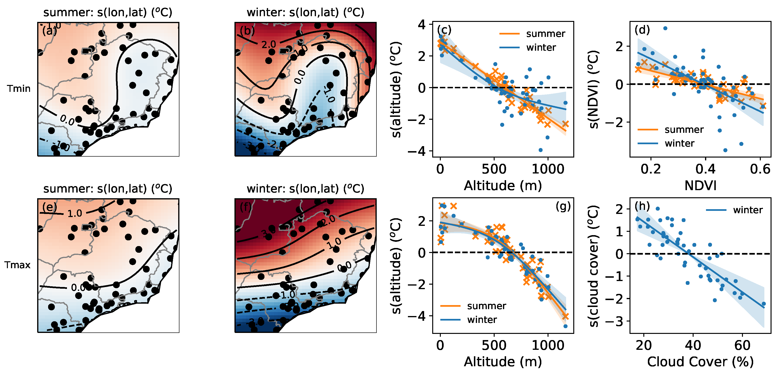
3.3. Seasonality of Gam Response

We further use GAM in a more detailed manner by fitting the summer and winter averages to see how the seasonality changes the estimated functions (Figure 6). For Tmin, the geographical position function, s(lon,lat), had a more significant contribution during winter, when horizontal gradients are more prominent, with a north-south difference of about 8 °C (Figure 6b), while in summer they are at most 3 °C (Figure 6a). For maximum temperature, the seasonality response was similar to Tmin, with meridional gradients above 8 °C in winter and lower than 3 °C in summer.
For the altitude function, we noticed little seasonal variation for Tmax (Figure 6g), where the lower sensitivity remains for altitudes that are lower than 500 m a.s.l., but with a steeper gradient above this altitude. For Tmin, we especially noticed that the dispersion around the fitted function was larger during winter than during summer, mostly in weather stations with an altitude lower than 500 m (Figure 6c). Kirchner et al. [39] and Li et al. [37] suggest that this is related to the increase of days with thermal inversions during winter, decreasing the lapse-rate. In fact, Martin et al. [35] showed that in small basins of meso- γ scale in Southeastern Brazil, the lapse-rate for Tmin is positive in the first 200 m of altitude, being more intense during winter, where it is limited by the thermal belt of the nocturnal boundary layer, and it becomes negative for altitudes higher than 200 m. It seems like this effect is incorporated in some of the analyzed stations, which helps to explain the pattern in winter(Figure 6c), but being difficult to quantify it.
The cloud cover functions were statistically significant only for winter (Figure 6h) and showed an amplitude of approximately 4 °C for cloud cover changes between 20 and 70%, comparable with the response from altitude and (lat,lon). The NDVI function for Tmin was significant for both seasons, with higher amplitude in winter (3 °C) than in summer (1.5 °C), even though there is a higher dispersion in winter (Figure 6e). Southeastern Brazil is characterized by dry winters and consequent lower cloud cover [43], also seen in Figure 6h, where values are mostly below 50%. This characteristic can potentially increase local contributions from vegetation and urbanization, with clear sky nights that are favorable to promote heating in urban areas (low NDVI) when compared to rural areas (high NDVI) [19].

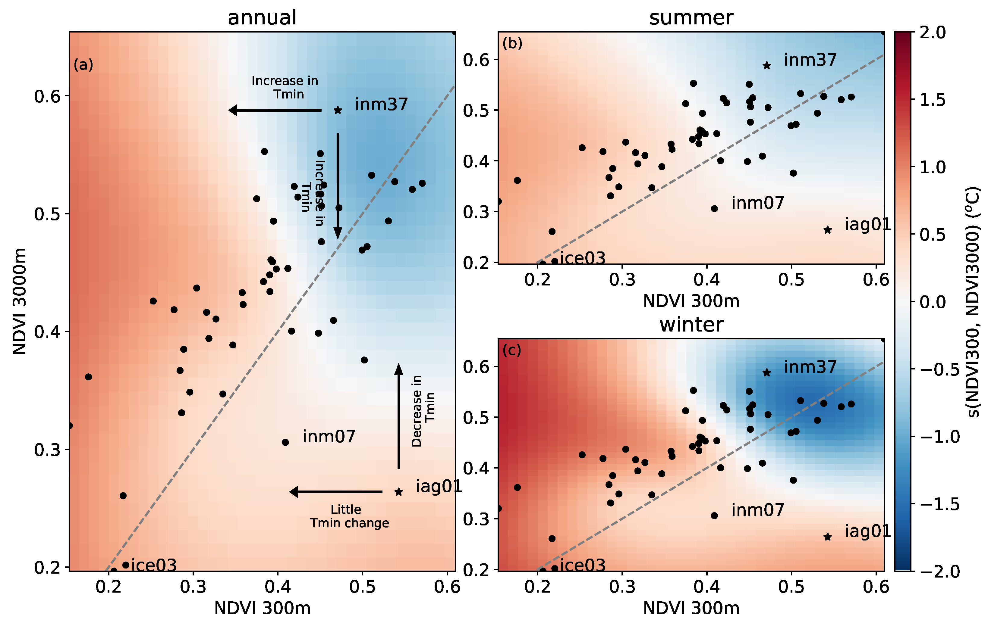
3.4. Impact of Land Use Heterogeneity in Urban Areas

As discussed in the previous sections, we found a correlation between minimum temperature and NDVI defined in a 300 m radius circle (hereafter referenced as NDVI300) and for Tmax but only in the SLR case, with no statistical significance in GAM and MLR. However, other factors may influence the signal’s amplitude, like wind speed which increases this spatial variability when wind speed is low (Section S4). There is also the possibility of contribution from urban heat islands that may extend up to 60 km from the city center [44], with great seasonal variability from parameters that are related to land cover and temperature of the order of 103 m [45].
According to [46], the spatial homogeneity of land cover up to the order of 103 m is important to evaluate the contributions from land use in urban temperature and urban heat island. Therefore, we reevaluated the spatial distribution of NDVI in an area of higher land cover spatial heterogeneity around the weather station. We take the example of the city of São Paulo, with a large urbanized area of 2310 km2, and two stations that are separated by a distance of approximately 4 km: iag01 (Figure 7a,b) located inside a park with more vegetation and higher NDVI, that is however surrounded by a densely urbanized area with lower NDVI; and ice03 (Figure 7a,c) station located in an airport with low NDVI in all surrounding area. On the other hand, we also identified two other stations, one at the north of SEB (inm07) (Figure 7a,d) and another one at the south (inm37) (Figure 7a,e) with different NDVI spatial distributions.
After finding differences in NDVI distribution, one of them in the same city, we reassessed the GAM for the prediction of average Tmin and Tmax, by considering the influence of NDVI by a smoother with multiple predictors using NDVI300 and NDVI3000 (NDVI defined in a 3000 m radius circle), referenced as s(NDVI300, NDVI3000). This term considers the local scale land use (NDVI300) and the regional scale (NDVI3000), which involves transport at the scale of the urban boundary layer. We chose the radius of 3000 m to capture the influence of the regional scale based on the leveling off of NDVI correlation with temperature, as noticed in Figure S4.
We fitted the GAM with s(NDVI300, NDVI3000), which was statistically significant for Tmin in all temporal aggregations, but not Tmax, similarly to the previous models using s(NDVI300) only. However, by using the term with multiple parameters, there was a best overall fit, with an increase of the explained variance from 93.4% to 96.1%, and a reduction in the BIC, from 127.2 to 123.7 (Table S4).
We did not notice a significant difference in the patterns associated with s(altitude) and s(lon,lat), but there are relevant applications to s(NDVI300, NDVI3000), as shown in Figure 8. The pattern of the function for the annual average Tmin shows negative values and colder weather stations (blue area in Figure 8a), which are dominated by high values of NDVI. In the opposite direction, the positive values represent warmer stations (red area in Figure 8a), that covers the entire range of NDVI. Still, in the annual average Tmin, in general, NDVI3000 was greater than NDVI300, as shown by the position of most stations distributed around the 1:1 line (Figure 8a). This implies that the areas closest to the station’s position have relatively lower green cover than the surrounding areas (up to 3000 m). There are few but important exceptions, like iag01 and inm08, that are relatively warm stations with high NDVI300, positioned in local areas with more vegetation than the surrounding areas (Figure 7b,d and Figure 8a). With respect to the seasonality of s(NDVI300, NDVI3000), the amplitude of the contribution was greater in winter, with approximately ±2 °C (Figure 8c), when compared to the summer, which was ±1 °C (Figure 8b).
An application of the function s(NDVI300, NDVI3000) is to verify how a hypothetical change in NDVI would contribute to altering the temperature in a given weather station. For example, shifting the station iag01 in the x direction (as displayed by the arrows in Figure 8a) by reducing the NDVI300 (keeping NDVI3000 constant), there is little temperature change, however, shifting it in the y direction and increasing NDVI3000 (keeping NDVI300 constant) leads to a decrease in temperature by reaching the blue part of the plot. Another example with a different result is the station inm37 which has high values of both NDVI300 and NDVI3000. In this case, a decrease in NDVI300 (keeping NDVI3000 constant) with changes in the x direction, increases temperature when reaching the warmer side of the plot, as well as a change in the y direction with a reduction of NDVI3000 (keeping NDVI300 constant). We used a large spatial domain to fit the model, that expresses the combined effects of a large sampling, and that might not be the ideal approach to detect changes at individual stations. Despite that, our simplified method used both the regional and local scale NDVI to suggest how the temperature relationship with NDVI depends on the heterogeneity of land-cover distribution across these scales.

4. Conclusions

With the purpose to assess the influence of local vegetation and regional scale geophysical controls on the spatial variability of near-surface temperature, we used 26 years of meteorological measurements from 52 conventional weather stations in Southeast Brazil. We used parsimonious statistical models of MLR and GAM, that helped to obtain the relationships of temperature with regional geophysical features (zonality, continentality, topography, and cloud cover) and local scale vegetation. The prediction of the average near-surface Tmax and Tmin showed the best overall performance with GAM, which used a single function to describe the combined effect of zonality and continentality, and for NDVI at local (300 m) and regional scale (3000 m).
Our results were generally consistent with the knowledge established in the literature. However, some studies relied on larger areas (up to 10 4 m of radius) due to uncertainties in the information of station position, to attribute relationships of land-use and near-surface air temperature [47,48]. As a novelty, our results fitted the dependency of geographical position and temperature with a non-linear method that represents the background climate conditions. Considering the additive property of the model we have on top of the spatial distribution, at least for Southeast Brazil, the land-use component, represented by NDVI, showed that, the variability of the near-surface air temperature is mostly correlated with local scale NDVI (300 m radius). Still, there is a combined effect of local vegetation with regional vegetation (3000 m) that represents the complexity of heterogeneous surfaces.
In GAM, the independent variables that accounted for the variation of the annual average Tmin were geographical position and altitude, each with an amplitude of ≃5 °C, and the NDVI that contributed with an amplitude of ≃3 °C. Similarly, the variables that accounted for Tmax variation were geographical position and altitude, each with an amplitude of ≃5 °C, and cloud cover that contributed with an amplitude of ≃3.5 °C. The seasonality of the amplitude of each fitted function was relatively small across variables, except for the geographical position and altitude in the Tmin model, which was slightly higher in winter compared to the annual mean.
Limitations of the proposed method are present, among them the fact that GAM is less generalizable than MLR, making it harder to extrapolate its results to other regions. Another limitation is the low density of stations available in the area that meet all required criteria for the analysis. The main geographical patterns are similar to those of Alvares et al. [16] and Rodríguez-Lado et al. [17], but a higher density is important for the characterization of the impact of land use heterogeneity. It would also help define more localized relationships with land use and topography, which would benefit from high-resolution data. For example, Local Climate Zones in the vicinity of the weather stations have information about architectural and urban morphology that are relevant to the surface energy budget [49], as well as topographic aspect and slope [23].
Finally, our results stress the need to clarify the causality of near-surface air temperature, at both the mean state and the temporal trends. Improving prediction of local temperature is key to adapting to global climate change and increasing urbanization. Especially in urban areas, it is recognized the need to achieve levels of climate resilience that assimilate current changes of the earth system. This issue can be driven partially through nature-based solutions [50,51], whereby public policies can design green spaces, using quantifying metrics that predict the possible effects distributed within in the urban space.

Supplementary Materials

The following supporting information can be downloaded at: https://www.mdpi.com/article/10.3390/atmos13111758/s1. References [12,19,52,53,54,55,56,57,58,59] are cited in the supplementary materials.

Author Contributions

Conceptualization, all authors; methodology, R.C.d.A. and H.R.d.R.; formal analysis, R.C.d.A.; investigation, R.C.d.A.; writing—original draft preparation, all authors; supervision, H.R.d.R.; funding acquisition, H.R.d.R. All authors have read and agreed to the published version of the manuscript.

Funding

This research was funded by Fundação de Amparo à Pesquisa do Estado de São Paulo (FAPESP) Grants 2015/50682-6 and 2019/23853-5, Coordenação de Aperfeiçoamento de Pessoal de Nível Superior/Agência Nacional de Águas e Saneamento Básico (CAPES/ANA) Grant 8887.144979/2017-00, and Coordenação de Aperfeiçoamento de Pessoal de Nível Superior—Brasil (CAPES) Finance Code 001.

Institutional Review Board Statement

Not applicable.

Informed Consent Statement

Not applicable.

Data Availability Statement

The data that support the findings of this study are openly available at https://doi.org/10.5281/zenodo.6927793, accessed on 28 July 2022.

Acknowledgments

We thank the employees from INMET, IAC, IAG, and ICEA institutes that made the data available and were open to answering any questions during the development of this research.

Conflicts of Interest

The authors declare no conflict of interest.

References

  1. Gulev, S.; Thorne, P.; Ahn, J.; Dentener, F.; Domingues, C.; Gong, S.G.D.; Kaufman, D.; Nnamchi, H.; Rivera, J.Q.J.; Sathyendranath, S.; et al. Changing state of the climate system. In Climate Change 2021: The Physical Science Basis: Working Group I Contribution to the Sixth Assessment Report of the Intergovernmental Panel on Climate Change; Allan, R., Collins, B., Eds.; Cambridge University Press: Cambridge, UK, 2021. [Google Scholar]
  2. Doblas-Reyes, F.J.; Sorensson, A.A.; Almazroui, M.; Dosio, A.; Gutowski, W.J.; Haarsma, R.; Hamdi, R.; Hewitson, B.; Kwon, W.T.; Lamptey, B.L.; et al. Linking global to regional climate change. In Climate Change 2021: The Physical Science Basis. Contribution of Working Group I to the Sixth Assessment Report of the Intergovernmental Panel on Climate Change; Masson-Delmotte, V., Zhai, P., Pirani, A., Connors, S.L., Pean, C., Berger, S., Caud, N., Chen, Y., Goldfarb, L., Gomis, M.I., et al., Eds.; Cambridge University Press: Cambridge, UK, 2021. [Google Scholar]
  3. de Abreu, R.; Tett, S.; Schurer, A.; Rocha, H. Attribution of Detected Temperature Trends in Southeast Brazil. Geophys. Res. Lett. 2019, 46, 8407–8414. [Google Scholar] [CrossRef] [Green Version]
  4. Jones, P.; Lister, D.; Osborn, T.; Harpham, C.; Salmon, M.; Morice, C. Hemispheric and large-scale land-surface air temperature variations: An extensive revision and an update to 2010. J. Geophys. Res. Atmos. 2012, 117, 1–29. [Google Scholar] [CrossRef] [Green Version]
  5. Bindoff, N.; Stott, P.; AchutaRao, K.; Allen, M.; Gillett, N.; Gutzler, D.; Hansingo, K.; Hegerl, G.; Hu, Y.; Jain, S.; et al. Detection and Attribution of Climate Change: From Global to Regional. In Climate Change 2013: The Physical Science Basis. Contribution of Working Group I to the Fifth Assessment Report of the Intergovernmental Panel on Climate Change; Stocker, T., Qin, D., Plattner, G.K., Tignor, M., Allen, S., Boschung, J., Nauels, A., Xia, Y., Bex, V., Midgley, P., Eds.; Cambridge University Press: Cambridge, UK; New York, NY, USA, 2013; Book Section 10; pp. 867–952. [Google Scholar] [CrossRef] [Green Version]
  6. Blain, G.C.; Picoli, M.C.A.; Lulu, J. Análises estatísticas das tendências de elevação nas séries anuais de temperatura mínima do ar no Estado de São Paulo. Bragantia 2009, 68, 807–815. [Google Scholar] [CrossRef] [Green Version]
  7. Marengo, J.A. Mudanças climáticas globais e regionais: Avaliação do clima atual do Brasil e projeções de cenários climáticos do futuro. Rev. Bras. Meteorol. 2001, 16, 1–18. [Google Scholar]
  8. Camilloni, I.; Barros, V. On the urban heat island effect dependence on temperature trends. Clim. Chang. 1997, 37, 665–681. [Google Scholar] [CrossRef]
  9. Kalnay, E.; Cai, M. Impact of urbanization and land-use change on climate. Nature 2003, 423, 528–531. [Google Scholar] [CrossRef]
  10. Wang, J.; Yan, Z.W. Urbanization-related warming in local temperature records: A review. Atmos. Ocean. Sci. Lett. 2016, 9, 129–138. [Google Scholar] [CrossRef] [Green Version]
  11. Ceppi, P.; Scherrer, S.C.; Fischer, A.M.; Appenzeller, C. Revisiting Swiss temperature trends 1959–2008. Int. J. Climatol. 2012, 32, 203–213. [Google Scholar] [CrossRef] [Green Version]
  12. Kagawa-Viviani, A.; Giambelluca, T. Spatial patterns and trends in surface air temperatures and implied changes in atmospheric moisture across the Hawaiian Islands, 1905–2017. J. Geophys. Res. Atmos. 2020, 125, e2019JD031571. [Google Scholar] [CrossRef]
  13. Hunt, J.D.; Stilpen, D.; de Freitas, M.A.V. A review of the causes, impacts and solutions for electricity supply crises in Brazil. Renew. Sustain. Energy Rev. 2018, 88, 208–222. [Google Scholar] [CrossRef]
  14. Nobre, C.; Young, A.F.; Saldiva, P.H.N.; Orsini, J.A.M.; Nobre, A.D.; Ogura, A.T.; Thomaz, O.; Párraga, G.O.O.; da Silva, G.C.M.; Valverde, M.; et al. Vulnerability of Brazilian megacities to climate change: The São Paulo Metropolitan Region (RMSP). In Climate Change in Brazil: Economic, Social and Regulatory Aspects; Motta, R.S., Hargrave, J., Luedemann, G., Gutierrez, M.B.S., Eds.; IPEA: Brasília, Brazil, 2011. [Google Scholar]
  15. Pereira, V.R.; Blain, G.C.; Avila, A.M.H.d.; Pires, R.C.d.M.; Pinto, H.S. Impacts of climate change on drought: Changes to drier conditions at the beginning of the crop growing season in southern Brazil. Bragantia 2017, 77, 201–211. [Google Scholar] [CrossRef] [Green Version]
  16. Alvares, C.A.; Stape, J.L.; Sentelhas, P.C.; de Moraes Gonçalves, J.L. Modeling monthly mean air temperature for Brazil. Theor. Appl. Climatol. 2013, 113, 407–427. [Google Scholar] [CrossRef]
  17. Rodríguez-Lado, L.; Sparovek, G.; Vidal-Torrado, P.; Dourado-Neto, D.; Macías-Vázquez, F. Modelling air temperature for the state of São Paulo, Brazil. Sci. Agric. 2007, 64, 460–467. [Google Scholar] [CrossRef] [Green Version]
  18. Silva Dias, M.A.; Vidale, P.L.; Blanco, C.M. Case study and numerical simulation of the summer regional circulation in São Paulo, Brazil. Bound.-Layer Meteorol. 1995, 74, 371–388. [Google Scholar] [CrossRef]
  19. Oke, T.R.; Mills, G.; Voogt, J. Urban Climates; Cambridge University Press: Cambridge, UK, 2017. [Google Scholar]
  20. Silva Dias, M.A.; Dias, J.; Carvalho, L.M.; Freitas, E.D.; Silva Dias, P.L. Changes in extreme daily rainfall for São Paulo, Brazil. Clim. Chang. 2013, 116, 705–722. [Google Scholar] [CrossRef]
  21. Zhao, L.; Lee, X.; Smith, R.B.; Oleson, K. Strong contributions of local background climate to urban heat islands. Nature 2014, 511, 216–219. [Google Scholar] [CrossRef] [PubMed]
  22. Manoli, G.; Fatichi, S.; Schläpfer, M.; Yu, K.; Crowther, T.W.; Meili, N.; Burlando, P.; Katul, G.G.; Bou-Zeid, E. Magnitude of urban heat islands largely explained by climate and population. Nature 2019, 573, 55–60. [Google Scholar] [CrossRef]
  23. Sun, R.; Zhang, B. Topographic effects on spatial pattern of surface air temperature in complex mountain environment. Environ. Earth Sci. 2016, 75, 621. [Google Scholar] [CrossRef]
  24. Wood, S.N. Generalized Additive Models: An Introduction with R; CRC Press: Boca Raton, FL, USA, 2017. [Google Scholar]
  25. WMO. A Note on Climatological Normals; Technical Report; World Meteorological Organization: Geneva, Switzerland, 1967. [Google Scholar]
  26. WMO. Guide to Instruments and Methods of Observation: Volume I—Measurement of Meteorological Variables; Technical Report; World Meteorological Organization: Geneva, Switzerland, 2018. [Google Scholar]
  27. Meek, D.; Hatfield, J. Data quality checking for single station meteorological databases. Agric. For. Meteorol. 1994, 69, 85–109. [Google Scholar] [CrossRef]
  28. Shafer, M.A.; Fiebrich, C.A.; Arndt, D.S.; Fredrickson, S.E.; Hughes, T.W. Quality assurance procedures in the Oklahoma Mesonetwork. J. Atmos. Ocean. Technol. 2000, 17, 474–494. [Google Scholar] [CrossRef]
  29. Beckers, J.M.; Rixen, M. EOF calculations and data filling from incomplete oceanographic datasets. J. Atmos. Ocean. Technol. 2003, 20, 1839–1856. [Google Scholar] [CrossRef]
  30. Henn, B.; Raleigh, M.S.; Fisher, A.; Lundquist, J.D. A comparison of methods for filling gaps in hourly near-surface air temperature data. J. Hydrometeorol. 2013, 14, 929–945. [Google Scholar] [CrossRef]
  31. Farr, T.G.; Rosen, P.A.; Caro, E.; Crippen, R.; Duren, R.; Hensley, S.; Kobrick, M.; Paller, M.; Rodriguez, E.; Roth, L.; et al. The shuttle radar topography mission. Rev. Geophys. 2007, 45, 1–33. [Google Scholar] [CrossRef] [Green Version]
  32. Wilson, A.M.; Jetz, W. Remotely sensed high-resolution global cloud dynamics for predicting ecosystem and biodiversity distributions. PLoS Biol. 2016, 14, e1002415. [Google Scholar] [CrossRef]
  33. Hastie, T.; Tibshirani, R.; Friedman, J. The Elements of Statistical Learning: Data Mining, Inference, and Prediction; Springer: Berlin/Heidelberg, Germany, 2009. [Google Scholar]
  34. Neter, J.; Kutner, M.H.; Nachtsheim, C.J.; Wasserman, W. Applied Linear Statistical Models; McGraw-Hill Irwin: Boston, MA, USA, 2005; Volume 5. [Google Scholar]
  35. Martin, T.C.; da Rocha, H.R.; Joly, C.A.; Freitas, H.C.; Wanderley, R.L.; da Silva, J.M. Fine-scale climate variability in a complex terrain basin using a high-resolution weather station network in southeastern Brazil. Int. J. Climatol. 2019, 39, 218–234. [Google Scholar] [CrossRef]
  36. Oliveira, A.P.d.; Silva Dias, P.L.d. Aspectos observacionais da brisa marítima em São Paulo. In II CBM: Anais 1980–2006; Sociedade Brasileira de Meteorologia: Rio de Janeiro, Brazil, 1982. [Google Scholar]
  37. Li, Y.; Zeng, Z.; Zhao, L.; Piao, S. Spatial patterns of climatological temperature lapse rate in mainland China: A multi–time scale investigation. J. Geophys. Res. Atmos. 2015, 120, 2661–2675. [Google Scholar] [CrossRef]
  38. Wallace, J.M.; Hobbs, P.V. Atmospheric Science: An Introductory Survey; Elsevier: Amsterdam, The Netherlands, 2006; Volume 92. [Google Scholar]
  39. Kirchner, M.; Faus-Kessler, T.; Jakobi, G.; Leuchner, M.; Ries, L.; Scheel, H.E.; Suppan, P. Altitudinal temperature lapse rates in an Alpine valley: Trends and the influence of season and weather patterns. Int. J. Climatol. 2013, 33, 539–555. [Google Scholar] [CrossRef]
  40. Wanderley, R.L.; Domingues, L.M.; Joly, C.A.; da Rocha, H.R. Relationship between land surface temperature and fraction of anthropized area in the Atlantic forest region, Brazil. PLoS ONE 2019, 14, e0225443. [Google Scholar] [CrossRef] [PubMed] [Green Version]
  41. Lambin, E.F.; Ehrlich, D. The surface temperature-vegetation index space for land cover and land-cover change analysis. Int. J. Remote. Sens. 1996, 17, 463–487. [Google Scholar] [CrossRef]
  42. Bhang, K.J. Anomalous variations of NDVI for a nonvegetated urban industrial area of Gumi, Korea. Am. J. Remote Sens. 2014, 2, 44–49. [Google Scholar] [CrossRef]
  43. Reboita, M.S.; Gan, M.A.; Rocha, R.P.d.; Ambrizzi, T. Regimes de precipitação na América do Sul: Uma revisão bibliográfica. Rev. Bras. Meteorol. 2010, 25, 185–204. [Google Scholar] [CrossRef]
  44. Hicks, B.B.; Callahan, W.J.; Hoekzema, M.A. On the heat islands of Washington, DC, and New York City, NY. Bound.-Layer Meteorol. 2010, 135, 291–300. [Google Scholar] [CrossRef]
  45. Suomi, J.; Hjort, J.; Käyhkö, J. Effects of scale on modelling the urban heat island in Turku, SW Finland. Clim. Res. 2012, 55, 105–118. [Google Scholar] [CrossRef] [Green Version]
  46. Stewart, I.D. A systematic review and scientific critique of methodology in modern urban heat island literature. Int. J. Climatol. 2011, 31, 200–217. [Google Scholar] [CrossRef]
  47. Wang, J.; Tett, S.; Yan, Z. Correcting urban bias in large-scale temperature records in China, 1980–2009. Geophys. Res. Lett. 2017, 44, 401–408. [Google Scholar] [CrossRef] [Green Version]
  48. Cao, W.; Huang, L.; Liu, L.; Zhai, J.; Wu, D. Overestimating impacts of urbanization on regional temperatures in developing megacity: Beijing as an example. Adv. Meteorol. 2019, 2019, 3985715. [Google Scholar] [CrossRef]
  49. Stewart, I.D.; Oke, T.R. Local climate zones for urban temperature studies. Bull. Am. Meteorol. Soc. 2012, 93, 1879–1900. [Google Scholar] [CrossRef]
  50. Mallick, S.K.; Das, P.; Maity, B.; Rudra, S.; Pramanik, M.; Pradhan, B.; Sahana, M. Understanding future urban growth, urban resilience and sustainable development of small cities using prediction-adaptation-resilience (PAR) approach. Sustain. Cities Soc. 2021, 74, 103196. [Google Scholar] [CrossRef]
  51. McClymont, K.; Cunha, D.G.F.; Maidment, C.; Ashagre, B.; Vasconcelos, A.F.; de Macedo, M.B.; Dos Santos, M.F.N.; Júnior, M.N.G.; Mendiondo, E.M.; Barbassa, A.P.; et al. Towards urban resilience through Sustainable Drainage Systems: A multi-objective optimisation problem. J. Environ. Manag. 2020, 275, 111173. [Google Scholar] [CrossRef]
  52. Wijngaard, J.B.; Klein Tank, A.M.G.; Können, G.P. Homogeneity of 20th century European daily temperature and precipitation series. Int. J. Climatol. 2003, 23, 679–692. [Google Scholar] [CrossRef]
  53. Alexandersson, H.; Moberg, A. Homogenization of Swedish temperature data. Part I: Homogeneity test for linear trends. Int. J. Climatol. 1997, 17, 25–34. [Google Scholar] [CrossRef]
  54. Pettit, A.N. A non-parametric approach to the change-point problem. Appl. Stat. 1979, 28, 126–135. [Google Scholar] [CrossRef]
  55. Verstraeten, G.; Poesen, J.; Demarée, G.; Salles, C. Long-term (105 years) variability in rain erosivity as derived from 10-min rainfall depth data for Ukkel (Brussels, Belgium): Implications for assessing soil erosion rates. J. Geophys. Res. Atmos. 2006, 111, 1–11. [Google Scholar] [CrossRef]
  56. El Kenawy, A.; López-Moreno, J.I.; Stepanek, P.; Vicente-Serrano, S.M. An assessment of the role of homogenization protocol in the performance of daily temperature series and trends: Application to northeastern Spain. Int. J. Climatol. 2013, 33, 87–108. [Google Scholar] [CrossRef] [Green Version]
  57. Menne, M.J.; Williams, C.N., Jr. Homogenization of temperature series via pairwise comparisons. J. Clim. 2009, 22, 1700–1717. [Google Scholar] [CrossRef] [Green Version]
  58. Xavier, A.C.; King, C.W.; Scanlon, B.R. Daily gridded meteorological variables in Brazil (1980–2013). Int. J. Climatol. 2016, 36, 2644–2659. [Google Scholar] [CrossRef] [Green Version]
  59. Souza, C.M., Jr.; Shimbo, J.Z.; Rosa, M.R.; Parente, L.L.; Alencar, A.A.; Rudorff, B.F.; Hasenack, H.; Matsumoto, M.; Ferreira, L.G.; Souza-Filho, P.W.; et al. Reconstructing three decades of land use and land cover changes in brazilian biomes with landsat archive and earth engine. Remote Sens. 2020, 12, 2735. [Google Scholar] [CrossRef]
Figure 1. (a) Minimum daily temperature (Tmin) trend for the stations in southeastern Brazil between 1985 and 2010, in °C 10 yr 1 , ordered from the lowest trend to the highest; (b) same as (a) but for daily average temperature (Tavg); (c) same as (a) but for maximum daily temperature (Tmax). Solid lines are the 95% confidence interval, vertical solid line is the average of all stations. * The dotted vertical line in (b) is the southeastern Brazil average temperature trend estimated from CRUTEM4 (Data from de Abreu et al [3]).
Atmosphere 13 01758 g001
Figure 2. Geographical position of the weather stations used in this research. Each station is identified by a colored point according to the different networks they belong (red: Instituto de Astronomia, Geofísica e Ciências Atmosféricas/Universidade de São Paulo (IAG); blue: Instituto Agronômico de Campinas/Secretaria de Agricultura e Abastecimento de São Paulo (IAC); orange: Instituto Nacional de Meteorologia (INMET); green: Instituto de Controle do Espaço Aéreo/Ministério da Aeronáutica (ICEA)). Shading represents the altitude in meters. Upper case and bold letters are the federal states delimited by the grey solid lines, and italic highlight the location of three important mountain chains: Serra do Mar, Serra da Mantiqueira, and Serra do Espinhaço.
Atmosphere 13 01758 g002
Figure 3. Flow chart of the main steps taken in the methods, including data source preprocessing, statistical methods (Simple Linear Regression (SLR), Multiple Linear Regression (MLR), and Generalized Additive Model (GAM)), and selecting the best model for the analysis.
Atmosphere 13 01758 g003
Figure 4. Scatter plot of the average annual maximum (red) and minimum (blue) temperature in each station, with the following independent variables: (a) latitude, (b) longitude, (c) altitude, (d) NDVI, (e) cloud cover. The solid line is the univariate linear regression fitted using ordinary least squares with the 95% confidence interval in shading. The equation and estimated parameters are located above each scatter plot, with the p-value of the scaling factor in parenthesis.
Atmosphere 13 01758 g004
Figure 5. Contribution of GAM terms, in °C, for the annual mean of Tmin (ac) and Tmax (df). In (a,d), is the function related to the geographical position s(lon,lat); in (b,e) is the altitude in meters above sea level (a.s.l.); (c) the NDVI and (f) the cloud cover in%. In (a,d) we show the position of each station used to fit the model. In (b,c,e,f): the points are the partial residual of the given function, and the fitted GAM response is displayed as a solid line with a 95% confidence interval.
Atmosphere 13 01758 g005
Figure 6. Contribution of GAM terms, in °C, for the seasonal mean of Tmin (ad) and Tmax (eh) for summer and winter. (ac,f) shows the geographical position, s(lon,lat); altitude in (c,g); NDVI in (d); and cloud cover in (h). In (ac,f) we show the position of each station used to fit the model. In (c,d,g,h): the points are the partial residual of the given function, and the fitted GAM response is displayed as a solid line with a 95% confidence interval.
Atmosphere 13 01758 g006
Figure 7. (a) Map of southeastern Brazil with all weather stations in this study, with a highlight for: iag01, ice03, inm08 e inm37; annual average NDVI (1985 to 2010) for: (b) iag01, (c) ice03, (d) inm08 e (e) inm37.
Atmosphere 13 01758 g007
Figure 8. Contribution from the s(NDVI300, NDVI3000) function from GAM, in °C, for minimum temperature in the following time aggregations: (a) annual, (b) summer, and (c) winter. The black dots represent the NDVI in each station, with the names highlighting the position of the stations given in Figure 7. The arrows indicate what happens when a given station is moved in the direction of the arrow (increase or decrease of NDVI). The dashed line is the 1:1 line, where NDVI300 = NDVI3000.
Atmosphere 13 01758 g008
Table 1. Estimated degrees of freedom (edf), and scaling factors β ^ j of each independent variable. R2 is the coefficient of determination, and BIC is the Bayesian Information Criteria. Only terms with p-value < 0.01 are displayed.
Generalized Additive Model (GAM)Multiple Linear Regression (MLR)
Tmax
(edf)
Tmin
(edf)
Tmax
β ^ j
Tmin
β ^ j
Intercept28.517.3Intercept37.527.5
---lon−0.17-
s(lon,lat)5.407.71lat0.440.26
s(altitude)1.951.55altitude−0.003−0.005
s(NDVI)-1.00NDVI-−6.04
s(cloud cover)1.56-cloud cover−0.10-
R294.3%93.4%R285.8%86.1%
BIC125.8127.2BIC155.4136.4
Publisher’s Note: MDPI stays neutral with regard to jurisdictional claims in published maps and institutional affiliations.

