Deep Learning Based Calibration Time Reduction for MOS Gas Sensors with Transfer Learning

Abstract

In this study, methods from the field of deep learning are used to calibrate a metal oxide semiconductor (MOS) gas sensor in a complex environment in order to be able to predict a specific gas concentration. Specifically, we want to tackle the problem of long calibration times and the problem of transferring calibrations between sensors, which is a severe challenge for the widespread use of MOS gas sensor systems. Therefore, this contribution aims to significantly diminish those problems by applying transfer learning from the field of deep learning. Within the field of deep learning, transfer learning has become more and more popular. Nowadays, building a model (calibrating a sensor) based on pre-trained models instead of training from scratch is a standard routine. This allows the model to train with inherent information and reach a suitable solution much faster or more accurately. For predicting the gas concentration with a MOS gas sensor operated dynamically using temperature cycling, the calibration time can be significantly reduced for all nine target gases at the ppb level (seven volatile organic compounds plus carbon monoxide and hydrogen). It was possible to reduce the calibration time by up to 93% and still obtain root-mean-squared error (RMSE) values only double the best achieved RMSEs. In order to obtain the best possible transferability, different transfer methods and the influence of different transfer data sets for training were investigated. Finally, transfer learning based on neural networks is compared to a global calibration model based on feature extraction, selection, and regression to place the results in the context of already existing work.

1. Introduction

The Global Burden of Diseases, Injuries, and Risk Factors Study (GBD) 2019 has shown that air pollution caused the premature death of around 6.7 million people in 2019 [1]. In order to lower the number of premature deaths, it is essential to analyze outdoor and indoor air regarding their toxic or harmful components. Since air generally consists of many different components, it is almost impossible to determine every substance within. Therefore, this contribution focuses on quantifying volatile organic compounds (VOCs), which are of great importance because there is a large variety of substances, some safe, like ethanol, and others highly toxic even at low concentrations like formaldehyde [2]. Today, only analytical measurement systems can quantify specific components (e.g., VOCs) with reasonable accuracy at the ppb level. However, these measurement systems are costly, require expert knowledge to operate, and are often not capable of real-time measurements. This prevents the widespread use of analytical measurements for reducing the risk associated with exposure to dangerous VOCs, especially in indoor air. One promising solution for a low-cost and easy-to-operate measuring system is provided by metal oxide semiconductor (MOS) gas sensors. Previous studies showed that such systems, together with complex operating modes and deep learning, can quantify single VOCs in complex environments at the ppb level [3]. The system, in this case, consists of one or multiple MOS gas sensors operated dynamically to obtain complex signal patterns. In particular, temperature cycled operation (TCO) has been demonstrated to greatly increase sensitivity, selectivity, and stability [4]. With the help of machine learning, a data-driven calibration model is built that analyses the complex sensor response patterns and can thereby predict gas concentrations of individual gases even in complex mixtures. However, due to even minute production tolerances of the gas sensing layer or the µ-hotplate for setting the temperature, it is necessary to calibrate every system individually, which requires several days to reach sufficient accuracy for complex gas mixtures. This greatly increases the cost and limits the widespread use of these advanced gas sensor systems. There are already transfer methods to significantly reduce the calibration time, such as direct standardization, orthogonal signal correction, global modeling, and many more, as shown in [5,6,7,8,9,10,11]. These methods calibrate a global model based on a few master sensors and use this for all additional sensors. In some cases, they also map the signals of additional sensors to the signals of the master sensors with the help of a few transfer samples. Thereby, the sensor signal of the new sensors is altered slightly to match the signal pattern of the master sensors. This allows for using the same global data-driven model with data from many different sensors. It was shown that those methods, together with a few transfer samples, can, for example, account for temperature differences caused by the hotplate or compensate for sensor drift. Nevertheless, those methods require that the sensor to be calibrated is operated under the exact same conditions, i.e., gas compositions and concentration ranges, during calibration as the master model. Thus, it is not possible to transfer models between different use cases. One promising solution for this problem might be transfer learning from the field of deep learning [12,13,14]. This method is often used for image classification tasks [15]. In this case, classification models are not built from scratch every time; instead, already existing models are adjusted to classify different objects in a picture.

This study adopts and applies transfer learning to data of a commercially available MOS gas sensor (SGP40, Sensirion AG, Stäfa, Switzerland). A deep convolutional neural network is trained on one master MOS gas sensor to build an initial model, which is then used as the starting point for other sensors to be calibrated. The gases analysed are the seven target VOCs acetic acid, acetone, ethanol, ethyl acetate, formaldehyde, toluene, and xylene, and the two background gases carbon monoxide and hydrogen, as well as the relative humidity. It was previously shown by [16,17] that it is possible to use such methods to reduce the calibration time of sensors significantly. To the best of our knowledge, not many scientific publications address deep transfer learning for gas sensor calibration; therefore, more research is required. Compared to the previous studies, we have tackled more complex situations, i.e., more than ten independent gas components with a focus on VOCs at low ppb concentrations are analyzed as a regression problem. The influence of different hyperparameters on transferability are investigated. For example, the influence of different transfer learning methods and the gases used for the transfer between sensors are analyzed. Furthermore, the results are compared with already existing work in the form of a conventional global calibration model based on feature extraction, selection, and regression.

2. Materials and Methods

2.1. Dataset

The dataset used throughout this study to evaluate the benefits of transfer learning in the field of deep learning is generated with our recently developed novel gas mixing apparatus (GMA), which allows up to 16 independent gases to be arbitrarily mixed over a wide concentration range. Details about this GMA are described in [18] and further details can be found in [19,20]. The GMA is used to provide well-known complex gas mixtures to three commercially available MOS sensors, i.e., SPG40 (Sensirion AG, Stäfa, Switzerland), with two sensors from one batch and the third from a different one. Every SGP40 holds four different gas-sensitive layers and is operated using temperature cycled operation (TCO) as shown in Figure 1. For this study, the temperature of sub-sensors 0–2 from all SGP40 is switched between high-temperature phases at 400 °C for 5 s, followed by low-temperature phases varying in 25-degree steps from 100 °C to 375 °C and lasting 7 s each. The temperature of sub-sensor 3 is only changed between 300 °C and 250 °C due to the lower temperature stability of this gas-sensitive layer. Each temperature cycle lasted 144 s with the logarithmic sensor resistance sampled at 10 Hz. Temperature cycling of the independent hotplates and read-out of the four gas-sensitive layers is achieved with the integrated electronic using custom software based on a protocol provided by Sensirion under a non-disclosure agreement. Further details are described in [19]. The data used for building the data-driven models always consists of one full temperature cycle of all gas-sensitive layers with the raw signal modified based on the Sauerwald-Baur model [21,22], i.e., a total of 5760 data points. For future reference, one complete temperature cycle is treated as an observation.

In order to calibrate the sensor for a complex environment, the gas mixtures applied by the GMA represent realistic gas mixtures as found in indoor environments consisting of eight different VOCs plus two inorganic background gases, CO and hydrogen. Furthermore, the relative humidity @20 °C is varied between 25–80%, resulting in a total of 11 independent variables. The eight VOCs chosen for calibration are acetic acid, acetone, ethanol, ethyl acetate, formaldehyde, isopropanol, toluene, and xylene, representing various VOC classes. They contain benign and hazardous VOCs (cf. Figure 2). During the experiment, multiple unique gas mixtures (UGMs) were randomly defined based on predefined concentration distributions. Latin hypercube sampling [23,24] was applied to minimize correlations between the different gases. All gas sensors were simultaneously exposed to these UGMs for several minutes to record multiple temperature cycles (TCs) or observations for each mixture. For Latin hypercube sampling, the experiment is divided into three different sections. For each of these segments, the concentration of every gas is randomly picked from a uniform distribution, cf.

Table 1. Concentration ranges for all target gases together with the number of unique gas mixtures (UGMs) for each range within the dataset.

	Segment 1 (1–200)	Segment 2 (201–500)	Segment 3 (501–906)
Carbon monoxide	100–2000 ppb	100–2000 ppb	100–2000 ppb
Hydrogen	400–2000 ppb	400–2000 ppb	400–2000 ppb
Acetic acid	1–50 ppb	1–150 ppb	1–500 ppb
Acetone	3–50 ppb	3–150 ppb	3–500 ppb
Ethanol	1–50 ppb	1–150 ppb	1–500 ppb
Ethyl acetate	1–50 ppb	1–150 ppb	1–500 ppb
Formaldehyde	1–50 ppb	1–150 ppb	1–300 ppb
Toluene	1–75 ppb	1–75 ppb	1–250 ppb
Xylene	2–150 ppb	2–150 ppb	2–500 ppb

. The specific gases and concentration ranges used for this study are based on [19,24,25].

In total, 906 UGMs were set, exposing all three SGP40 sensors simultaneously for approx. 10 TCs (1440 s), yielding an overall calibration duration of more than 15 days. Because of synchronization problems between GMA and the sensors’ data acquisition, only three to four TCs or observations per UGM are used for further evaluation. The target for the data-driven models is an accurate prediction of the gas concentration for each gas, VOC, or inorganic background gas individually. As an additional target, the sum concentration of all VOCs within the mixtures is also predicted as this TVOC_sens value might be a suitable indicator for indoor air quality. Because of minimal sensor response to isopropanol, it is excluded as an independent target and contributor to the TVOC_sens target.

This dataset consists of the data of three SGP40 sensors. Throughout this study, sensor A will be used to build the initial models from which the calibration models for sensor B (same batch) and sensor C (different batch) are derived. Sensors from different batches have been chosen to investigate the effect of transferring a data-driven model across batches, as one would expect larger differences in sensor parameters. Sensors A and B are from the same batch, and sensor C is from a different one.

2.2. Model Building and Methods

A ten-layer deep convolutional neural network (TCOCNN [3]) is used to derive the data-driven model (cf. Figure 3). The input for this neural network is one observation represented in a 4x1440 array. The first dimension describes the different gas-sensitive layers per sensor, and the second dimension covers the time domain (144 s sampled at 10 Hz). In previous studies, it is shown that this TCOCNN achieves similar or slightly better results than classical approaches based on feature extraction, selection, and regression (FESR) [3] and can be used for transfer learning [16]. Other contributions also showed that neural networks can be used to calibrate gas sensors and achieve similar results to established methods [26]. The focus of this contribution will be on the TCOCNN from [3] as a starting point for transfer learning. This will also include the normalization of the input matrix. Currently, this is done by calculating the mean and standard deviation of the complete 4 × 1440 matrix of one observation and then normalizing this frame. This standard approach for pictures is not the best for sensor-based data, where normalization would ideally be done for each sub-sensor.

The hyperparameters of the neural network are optimized independently for each analyzed gas, similar to the optimization done in [3]. Hyperparameter tuning of the TCOCNN is performed with Bayesian optimization and neural architecture search (NAS) [27,28]. The optimized parameters are the initial learning rate of the optimizer, the number of filters, and kernel size, and striding size of the convolutional layers, the dropout rate, and the number of neurons of the fully connected layer. The optimization for all sensors is based on sensor A and is performed on 500 randomly chosen UGMs (450 for training and 50 for validation). The optimization goal was to minimize the root-mean-squared error (RMSE) on the validation data as described in [3]. In our typical workflow, the final model would be trained for each individual sensor from scratch after hyperparameter tuning with 700 UGMs and tested on the remaining 200 UGMs.

Figure 3. Architecture of the TCOCNN neural network (adapted from [29]).

Figure 3. Architecture of the TCOCNN neural network (adapted from [29]).

2.2.1. Transfer Learning

In order to improve the training process of the TCOCNN, primarily by reducing the number of UGMs required for calibration, transfer learning is now introduced [12,13,14,15]. Transfer learning in the scope of deep learning is generally used to adapt the information of an already existing model to a new task or a new domain. For neural networks, this information is stored within the weights and biases, as they are used to transform the input to form the output. Therefore, they contain information on the dependencies between input and output. Thus, those weights and biases can be used for a similar task and must only be adjusted with additional training. The exact definition of transfer learning and how it is used with and without deep learning can be seen in multiple surveys [30,31,32]. In our case, we want to maintain the information within the weights and biases about interpreting different signal patterns for specific gas concentrations and transfer this information to other sensors [16]. This is done by not initializing the model with random weights and biases. Instead, the weights and biases from a previously calibrated network (different sensor or sensors) are used as a starting point (initial/global model). This ensures that the neural network starts not without any information about the task at hand. This means that, before the training/calibration starts for the new sensor, the neural network contains information on how to transform the input. Nevertheless, a further adjustment of the weights and biases in the form of additional training is necessary because of production differences between every sensor (new domain).

The benefits of transfer learning can be seen in Figure 4. This scheme was initially proposed for classification by [12] and is here adapted to a regression problem for gas sensor calibration. It shows that, with proper transfer learning together with suitable data, it is possible to improve the starting accuracy, increase the learning slope, and perhaps even achieve better results than the initial model. However, it is also illustrated that the amount of data, here the number of UGMs, and the transfer learning method are essential to achieve the desired improvement. An improvement means either reaching an acceptable accuracy, here a required measurement uncertainty expressed as RMSE, with fewer data, or achieving higher accuracy with a similar amount of data. This study will analyze both possible improvements for our use case.

In order to transfer the gas sensor calibration from one sensor (sensor A) to one of the others (sensor B or C), multiple methods are available, which were used for other data-driven problems, like computer vision or speech recognition [15,33]. Throughout this contribution, four different methods for transfer learning will be tested. Three of them belong to the field of fine-tuning [34], where not only certain parts of the model are retrained, but the whole model is adjusted to the new domain (e.g., sensor), which means that every weight and bias is readjusted. Those three fine-tuning methods vary in the rate the network parameters are allowed to change, which the initial learning rate can control. The lower the initial learning rate, the less the parameter within the network will change. Method one sets the initial learning rate to the learning rate the TCOCNN has reached at the end of the training of the initial model, which is low because, during TCOCNN training, the learning rate is decreased after every two epochs by 0.9. The second method sets the initial learning rate to the value reached halfway through the initial training process, while the third set the learning rate to the value at the beginning of the initial training. On the other hand, the fourth method keeps all parameters of the convolutional layers fixed and only adapts the parameters in the last two fully connected layers to the new sensors [34]. Thus, this method basically keeps the implicit feature extraction [35] as derived for the model of sensor A and only retrains the regression part of the network. This allows for gaining insights if an adaptation of the implicit feature extraction is necessary for new sensors.

2.2.2. Global Model

After introducing transfer learning, it is also important to compare this method with already existing approaches like global model-building [7]. Here, a global model-building approach means one model trained once on all available data samples, i.e., covering different gas sensors. Based on this definition, the transfer learning approach based on neural networks, as introduced above, is not a global calibration method, as individual models for different sensors are obtained. For practical application, a comparison between transfer learning and global modeling is important as a valid global model would completely eliminate the necessity for individual gas sensor calibration. In this case, we chose not to compare this with neural networks but instead used established methods based on feature extraction, selection, and regression (FESR). Usually, we use this approach only on single sensors, as shown in [19], but this approach is extended to multiple sensors in this study. As for the neural network, the data is split into 700 UGMs for model building and 200 UGMs for testing data. For feature extraction, adaptive linear approximation (ALA) is used. This extraction method divides the raw signal into sections and calculates the mean and slope of these sections as features. The segmentation is optimized based on the reconstruction error on the full training set that is achieved with the calculated mean and slope values. Details are given in [36,37]. The feature selection is performed with 10-fold cross-validation (based on all observations) of the training data. In this case, the training set is split randomly into ten parts, and the RMSE is calculated for the different training sets (different numbers of features) across all folds. First, the features are sorted based on their Pearson correlation to the target gas to reduce the number of features to a manageable level, here 200. Then, the feature set is gradually increased from 1–200 features. The resulting sets are tested with the help of a partial least squares regression (PLSR) with a maximum of 100 components [38,39], and the set with the smallest RMSE across all ten folds is used for later evaluations (e.g., [37]). The final regression is then built with the help of a PLSR with a maximum of 100 components and the data available from multiple sensors.

2.3. Data Evaluation

In order to evaluate the capabilities of transfer learning, this section summarises the strategies followed to test transfer learning. Before any evaluations are performed, the data are split into training (700 UGMs) and testing (200 UGMs) data. The 200 test UGMs are the same throughout all evaluations and also for different sensors to make the comparison fair.

As stated in the modeling section, the TCOCNN is first optimized for the different gases. In addition, 500 random UGMs are picked from the 700 available training UGMs from sensor A. The Bayesian optimization is then performed with 450 UGMs for training and 50 for validation. The model parameters that achieve the lowest validation RMSE are then chosen for the rest of this contribution for the specific gas. A detailed explanation of this process can be found in [3], albeit for a different sensor model.

In the next step, the RMSE that these models can achieve is determined, i.e., the RMSE when training the model with the selected hyperparameters with all 700 training UGMS and testing on the 200 independent test UGMs. This training process is repeated ten times for every gas and for all sensors to determine the stability of the achieved models. The mean RMSE values of the training are used as reference RMSE values for the subsequent transfer learning.

In the first part, different methods for transfer learning are studied and compared. Thus, an initial model is built based on the 700 training UGMs for sensor A. Since this model building was already performed in the previous step for calculating the baseline ten times, the model picked for transfer is the last model built during the baseline calculation. With this model and a subset of the UGMs (“transfer samples”), the performance of the four different transfer learning methods is tested to analyze which method(s) work best for specific gases. The main question is how many transfer samples are required to reach an acceptable accuracy. This is analyzed by varying the number of transfer samples from 20 to 700 UGMs, i.e., up to the full data set of the original training. Furthermore, the methods are tested for sensors B and C to analyze their performance for sensors from the same and from a different batch. The metric to compare the different methods and the number of training samples is the RMSE reached on the test data set, i.e., the 200 testing UGMs, which are always the same regardless of which scenario is tested. All pieces of training are performed multiple times to gain insight into the stability of the tested approach. The paper presents the results for only a few relevant gases, and the remaining results are shown in Appendix A.

The second part then compares the best model achieved by transfer learning and a model built from scratch. Therefore, the accuracy in terms of RMSE of the models with transfer learning and no transfer learning are compared across all sensors. This gives an overview of the benefits transfer learning can provide. As for the first test scenario, the number of samples used for training varies from 20 to 700. Furthermore, the influence of the specific samples used for training the models is compared by randomly picking 20–500 training samples from the 700 available samples and training each specific case 10 times to estimate the variation caused by different training sets (random subsampling). In order to compare this variation with the variation during normal training with a fixed set, a static training set is also trained ten times. This allows for estimating how much variation is caused by the neural network itself and how much by the random subsampling.

In order to confirm the achieved results from the previous sections, the experiments are repeated with an optimized standardization of the raw data and the different transfer strategies. For this experiment, the raw signal of each of the four sub-sensors is normalized independently for each temperature cycle as the raw signals of the sub-sensors differ significantly because of the gas-sensitive materials and the different temperature ranges. This experiment shows that the general method is always applicable when used with a different normalization for the neural network.

The last part of the results compares the transfer learning approach with a simplified global calibration approach based on established methods like feature extraction, selection, and regression. Similar to the neural network approach, the data of all sensors are based on the same split of the data set into training (700 UGMs) and test data (200 UGMs) as for the evaluation above. As mentioned above, the feature extraction is based on the adaptive linear approximation. The feature selection is performed by finding the optimal subset of Pearson sorted features based on the validation set (10-fold cross-validation). In order to test this method as a global calibration scheme, all training UGMs of one sensor, together with additional samples from another sensor, are used to build the model. Here, the same evaluations as for the neural networks are performed: Models are trained with 700 UGMs from sensor A together with 20–700 additional samples from sensor B and tested on the 200 test UGMs from sensor B. Finally, the evaluation with 20–500 randomly selected UGMs is repeated ten times to evaluate the influence of different training sets also for the global approach.

The previously described evaluation steps are visualized in Figure 5, to make the process easier to understand.

3. Results

Before the transfer methods can be compared, the reference values must be obtained to rate the transfer methods (cf. Figure 6). The mean RMSE values for sensors A and B are very similar for the different gases. The largest difference regarding the achieved RMSE divided by the mean concentration of the specific gas is observed for ethanol, where the relative RMSE for sensor A is 3.2% smaller than sensor B. Thus, the hyperparameter tuning performed to find an optimized architecture for a specific gas based on sensor A can also be used as architecture for other sensors from the same batch. For some gases, sensor B outperforms sensor A, although the network was not optimized for this specific sensor. On the other hand, the performance of sensor C (different batch), while comparable for some gases with RMSE values close to the sensors A and B, is significantly reduced for acetone and hydrogen compared to the other sensors. This effect cannot be attributed to sensor drift as sensor C was used over a similar period as the other two. The most probable explanation for the observed difference could therefore be a slight variation of one or more gas-sensitive layers between the batches.

As already used above, another important measure to rate the quality of the TCOCNN is the RMSE divided by the mean concentration. Here, the best result is achieved for hydrogen with a deviation of only 4%, the average deviation for the other gases is between 10 and 30%, which is still a reasonable result that can be useful for IAQ applications. One exception is toluene. For this gas, the deviation is 45%, which is still useful but not as promising as the other gases. Nevertheless, the RMSE of this gas can be significantly reduced with the adapted normalization (21.7 ppb), and a reasonable RMSE divided by the mean concentration of 28.6% can be achieved. Thereby, it can be stated that the TCOCNN can be a useful tool for calibrating gas sensors.

Figure 7 shows the results of the first test scenario where different transfer learning methods are compared. The results are shown exemplarily for carbon monoxide and formaldehyde, two gases that are of great importance for air quality assessments. Carbon monoxide was chosen because of its toxic properties and also because it is a ubiquitous background or interfering gas when monitoring VOCs. Formaldehyde was chosen because of its carcinogenic properties even at low concentrations [2]. Within Figure 7, the dashed lines indicate the accuracy achieved with different transfer methods over the number of training UGMs. The solid lines indicate the best RMSE achieved without transfer learning using 700 UGMs over ten trials. For sensor B and carbon monoxide, transfer method 2 (learning rate between min and max) performs best across all different transfer sets. Method 1 (initial learning rate at minimum) performs similarly well for small transfer sets, while method 3 (initial learning rate at maximum) performs slightly better for very large transfer sets. Similar behavior can be observed for formaldehyde, where methods 1 and 2 are very similar for small transfer sets, while methods 2 and 3 yield almost identical results for larger transfer sets. For carbon monoxide and formaldehyde, it can be seen that transfer method 4 (static feature extraction) performs worst, at least for larger transfer sets. That allows the assumption that, although the different sensors achieve similar performance for the full dataset when trained from scratch (Table 1), they rely on slightly different features. Therefore, the implicit feature extraction, as well as the regression within the fully connected layers, needs to be transferred between models. Method 4 achieves competitive results only for formaldehyde and very small transfer sets with 20 UGMs. Furthermore, it can be observed that method 3, especially for small transfer sets (e.g., 20 UGMs), shows a large variation of the RMSE values. Thus, the method lacks robustness. This behavior is not observed for the other methods, which allows the interpretation that learned dependencies could be maintained more easily when reducing the initial learning rate for the parameters of the TCOCNN. This behavior for method 3 is counterproductive to the general goal of this contribution. Since we want to reduce the calibration time, achieving good models for small transfer sets is the highest priority. Thus, method 2 seems to be the most promising transfer method for further evaluation. Nevertheless, one should note that method 3 outperforms all other methods for all gases when used with the full 700 UGM transfer sets. For this scenario, method three, on average, achieves results even better than the absolute best RMSE obtained for the different gases without transfer learning. This shows that pre-trained networks can improve the accuracy of different sensors even when not reducing the calibration time, apparently by using the additional information contained in measurements of other sensors. Here, results of only the most relevant gases are presented. Results of the remaining gases are provided in Appendix A.

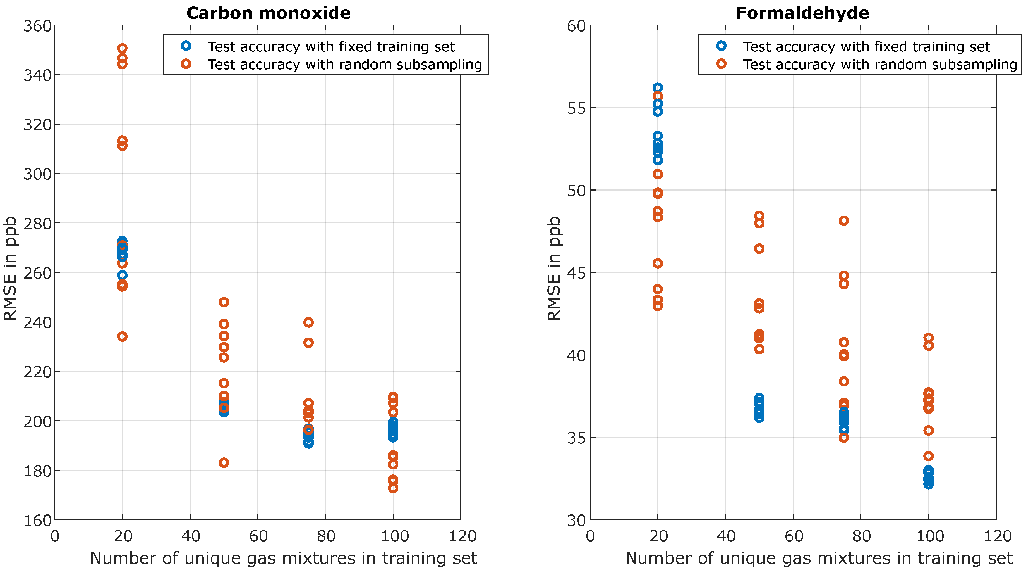
To compare the benefits of transfer learning with results when models are trained from scratch, Figure 8 shows the comparison of transfer method 2 for sensors B and C together with a model trained from scratch on sensor A, again for the two relevant target gases carbon monoxide and formaldehyde. The solid lines within the figures indicate the best possible RMSE achieved with 700 UGMs over ten tries and are used as a reference for all further evaluation. The dashed blue curve illustrates the achieved accuracy for sensor A, i.e., when no transfer learning is applied, while the dashed orange and yellow lines show the results achieved with transfer learning. In order to capture the variance caused by the different UGMs used in the training set, the standard deviation is marked for all sensors and training sets. The blue line, i.e., sensor A without prior information, always starts at much higher RMSE values than the yellow and orange lines for sensors B and C with transfer learning and also shows a larger standard deviation. This implies that the quality of the results is significantly improved when applying transfer learning, as the models reproducibly achieve better accuracy. Furthermore, for both gases, the benefit of transfer learning is most significant when applied to sensors from the same batch. This is demonstrated by the orange line (sensor B), which is significantly lower than the yellow line (sensor C) and exhibits a smaller variance similar to results reported previously [16]. This is plausible as the difference in terms of both the various gas-sensitive layers and the µ-hotplate should be much smaller between sensors A and B compared to sensor C. Note, however, that the performance of sensor C is not as good as for sensors A and B also when trained from scratch. Overall, all training curves converge towards the best possible model achieved with 700 UGMs without transfer learning, with sensor B achieving a slightly lower RMSE for formaldehyde with additional transfer learning compared to training the model from scratch. Note that this demonstrates that more than 700 UGMs would not improve the accuracy significantly, indicating that 700 UGMs are sufficient even for the complex gas mixtures (10 gases plus humidity) studied here.

In conclusion, it can be stated that transfer learning can significantly reduce the required calibration time by up to 93%, i.e., 50 UGMs instead of 700, while increasing the RMSE only by approx. a factor of 2 even for sensors from a different batch. In practical applications, the possible calibration time reduction will depend on the required performance, i.e., the acceptable RMSE for a specific use case.

After the general findings are discussed above,

Table 2. Detailed RMSE values for carbon monoxide and formaldehyde for Figure 8 with a static training set or training set with random subsampling.

	Carbon Monoxide in ppb			Formaldehyde in ppb
	Sensor A	Sensor B (Transfer)	Sensor C (Transfer)	Sensor A	Sensor B (Transfer)	Sensor C (Transfer)
700 UGMs mean RMSE (std)	110.9 (4.1)	121.1 (1.6)	147.3 (3.0)	23.6 (1.4)	21.2 (0.4)	29.4 (0.3)
Initial model before transfer		532.3	782.9		55.1	73.0
75 UGMs mean RMSE (std) static training set	332.6 (8.4)	194.3 (1.9)	256.3 (2.3)	67.0 (2.5)	36.1 (0.5)	44.4 (0.4)
75 UGMs mean RMSE (std) random subsampling	359.4 (37.8)	206.8 (16.0)	264.7 (26.3)	75.5 (9.5)	36.6 (2.3)	48.9 (6.0)
50 UGMs mean RMSE (std) static training set	374.8 (7.3)	206.0 (1.5)	238.1 (2.8)	76.1 (0.9)	36.8 (0.4)	46.7 (0.2)
50 UGMS mean RMSE (std) random subsampling	392.5 (39.2)	219.8 (19.3)	285.6 (23.3)	76.8 (8.0)	38.5 (3.2)	52.1 (4.9)
20 UGMs mean RMSE (std) static training set	856.4 (8.0)	268.3 (3.9)	349.1 (2.8)	80.3 (1.4)	53.3 (1.5)	72.4 (2.4)
20 UGMS mean RMSE (std) random subsampling	831.9 (19.3)	294.4 (43.8)	362.1 (31.6)	95.6 (23.5)	50.8 (6.1)	64.6 (8.8)

provides quantitative values for carbon monoxide and formaldehyde. Considering the ambient threshold limit value for CO of 10 mg/m³ [40], corresponding to approx. 8.5 ppm, the accuracy achieved with small transfer sets is excellent and significantly lower than a model generated from scratch without transfer learning, as shown for sensor A. Similarly, for formaldehyde, the WHO limit of 80 ppb [41] could be monitored with sensors trained by transfer learning on small calibration data sets.

Furthermore, Table 2 and Figure 9 also demonstrate the effect of different sets of transfer samples for transfer learning. The static sets, where the training was repeated ten times with the same data sample, always show a slightly smaller mean RMSE with a much smaller variation than the training set with random subsampling. In the example shown, it seems the randomly chosen static training sets for formaldehyde and carbon monoxide were a lucky choice as they resulted in a lower mean RMSE. More significant is the standard deviation, which is significantly larger for the training sets with random subsampling. It seems clear that the changing UGMs cause additional variance within the training sets. A closer look at Figure 9 shows that a poor choice for 75 transfer samples results in a higher RMSE for CO (207 ppb plus 16 ppb) than a good choice for 50 UGMs (220 ppb minus 19 ppb). This indicates that the choice of samples for transfer learning is important to obtain the best possible results, i.e., even shorter calibration times or better performance with the same calibration time. When analyzing the distribution of the different training sets, a good training set is usually signified by samples spanning the full concentration range of the target gas. However, the distributions of other gases are also relevant for the achieved performance. Therefore, the design of experiment (DoE) for optimal transfer learning-based calibration is a topic for future research.

The analysis is repeated for sensor B using the adapted normalization strategy with the results shown in Figure 10 for formaldehyde and xylene. Formaldehyde was chosen to have one example throughout this study, and xylene was selected because the difference between both normalization strategies was one of the largest. The figure shows the former and the adapted normalization results in the upper and lower part, respectively. The best RMSE for formaldehyde achieved with the adapted normalization is slightly better, and the improvement for xylene is significant with a reduction of the RMSE of 25%. Thus, normalization substantially impacts model building, and a suitable normalization can significantly improve the ML model accuracy. At the same time, the general shape of the improvement in accuracy with an increasing number of transfer samples is very similar for both gases, independent of the applied normalization. The obtained models can yield slightly higher or even lower RMSE values for both scenarios depending on the transfer method. The ranking of the different transfer methods is the same, and in each case, transfer method two achieves the best overall results. The only significant difference is the smaller mean RMSE achieved with the adapted normalization, which can be attributed to the improved preprocessing allowing for a better model accuracy. This result shows that the findings for the transfer learning method might apply not only to this specific example but might also be a suitable approach for transfer learning for gas sensors in general.

Again, as for the former normalization, the models obtained with transfer learning show a better performance than without both in terms of overall accuracy and training stability as indicated by the standard deviation (cf.

Table 3. RMSE values together with the standard deviation for the adapted normalization with and without transfer learning for formaldehyde and xylene.

Mean RMSE (std) in ppb	20 UGMs	50 UGMs	75 UGMs	100 UGMs	150 UGMs	500 UGMs
Without transfer learning (formaldehyde)	87.6 (10.4)	78.5 (3.3)	72.0 (9.3)	61.0 (6.7)	40.3 (5.2)	21.0 (1.0)
Transfer method 2 (formaldehyde)	39.6 (3.2)	34.0 (4.2)	35.6 (5.1)	26.9 (1.0)	26.6 (2.0)	19.9 (0.6)
Without transfer learning (xylene)	65.4 (5.6)	50.9 (9.1)	38.1 (2.0)	32.4 (1.9)	26.5 (1.4)	20.0 (0.5)
Transfer method 2 (xylene)	34.8 (3.7)	26.1 (1.7)	25.5 (0.9)	24.7 (1.6)	22.9 (1.0)	18.8 (0.7)

).

Finally, we compare results achieved with transfer learning (here with the former, sub-optimal normalization) and a simplified global model. Figure 11 shows the RMSE achieved for formaldehyde for the two models when trained with the same number of UGMs recorded with two different sensors (sensor A, sensor B) and tested on the same test data. First, the solid lines indicate the best possible RMSE achieved when training with only 700 UGMs from sensor A and testing with the test data (200 UGMs) also from sensor A. In this scenario, the TCOCNN (21.1 ppb) performs slightly better than the established FESR methods (25.9 ppb), but this also depends on the target gas, and in general, the performance achieved with both methods is comparable as demonstrated previously [3]). The dashed lines indicate the accuracies achieved with the additional samples from sensor B and tested with data from sensor B. Comparing the general trend and the standard deviations, both approaches are quite similar regarding the number of UGMs. Thus, additional samples from the new sensor can improve the prediction quality for the global model and the neural network. The selection of UGMs (DoE) is most important for achieving a low RMSE. Furthermore, in the stages between 20 and 100 UGMs, the differences between both approaches are very small. They can most probably be attributed to the slightly better initial accuracy of the transfer learning model. The largest difference is observed if both models are trained with 700 additional UGMs. In this case, the transfer model converges towards the best possible RMSE while the global model settles at a higher RMSE. This can be attributed to the generalization of the global model, which builds the best possible model for both sensors simultaneously, thus not achieving the lowest RMSE for a sensor-specific model. For transfer learning, on the other hand, the new model is specifically adapted to the new sensor B and will therefore show a higher RMSE for the original sensor A (84.4 ppb). A larger dataset with more sensors is required to compare the pros and cons of individual transfer learning and global modeling more in-depth. In addition, methods for signal correction like direct standardization or orthogonal signal correction should be analyzed in this context [5,6].

4. Discussion

This paper demonstrates that a significant reduction of the calibration time for accurate quantification of multiple gases at a ppb level within complex environments is possible with transfer learning. Various methods of transfer learning can be applied to reduce the training time. This study achieved the best results with transfer method 2 (complete adaptation of all CNN parameters with initial learning rate for transfer learning set to the value reached halfway through the original model training). This allowed a reduction of 93% (50 instead of 700 unique gas mixtures) while increasing the RMSE by less than a factor of 2. However, the optimal method cannot be generalized as this will vary according to the specific sensor model, the target gas, and the use case, i.e., concentration range and interfering gases. Furthermore, we could show that transferring data-driven models from one sensor to another always results in better accuracy than building the models from scratch, both when analyzing long or short calibration times. Again, the number of transfer samples required for building an acceptable data-driven model will vary, i.e., between sensors from different batches, and also strongly depends on the required accuracy. Furthermore, the influence of varying transfer samples was analyzed, which demonstrated that transfer learning could only develop its full potential if the transfer samples were selected with care. However, the selection of suitable samples is not straightforward and not yet fully understood. However, it would seem reasonable to follow the same rules as for the design of experiments in ML model building in general. Finally, transfer learning was compared with global modeling. For the small dataset with only two sensors studied here, we could show that both model-building approaches (transfer learning and global modeling) yield reasonably similar results, especially when using only a few additional samples from a second sensor. When using the entire dataset, the differences between transfer learning and global modeling become evident, i.e., transfer learning achieves a higher accuracy for a sensor-specific model, while global modeling yields greater generalization for different sensors. For a more in-depth analysis of the benefits and drawbacks of both methods, a larger dataset with multiple different sensors is required.

5. Conclusions

In conclusion, transfer learning can be used to significantly reduce the calibration time of MOS gas sensors by up to 93% while maintaining an RMSE that is only double the best possible. It was shown that different transfer methods provide additional benefits and drawbacks and that the selection of UGMs is most important. Nevertheless, a suggestion of which method or UGMs to use could not be made because this highly depends on the use case. Finally, we compared deep transfer learning with the global modeling approach. We found that deep transfer learning performs similarly to global modeling, although it might be essential to analyze this comparison in more detail with a larger dataset (multiple sensors).

For further research, it might be interesting to not only use a single sensor to build the initial model but to use a global calibration model based on multiple sensors and combine this approach with transfer learning. Furthermore, a wider variety of transfer methods should be tested and compared with deep transfer learning, as proposed in this work. Likewise, transfer learning should include methods from deep learning and extend to complementary approaches such as direct standardization or other signal-related transfer methods. This would also allow for combining different datasets with only one or few (target) gases in common but different backgrounds. This could help analyze the transferability between backgrounds and improve the understanding of which gases interfere with each other on the sensor.