Article

Simulation of the Dynamic and Thermodynamic Structure and Microphysical Evolution of a Squall Line in South China

1
Laboratory of Cloud-Precipitation Physics and Severe Storms (LACS), Institute of Atmospheric Physics, Chinese Academy of Sciences, Beijing 100029, China
2
University of Chinese Academy of Sciences, Beijing 100049, China
3
Ningxia Hui Autonomous Region Meteorological Bureau, Yinchuan 750002, China
4
College of Atmospheric Sciences, Nanjing University of Information Science and Technology, Nanjing 210044, China
*
Author to whom correspondence should be addressed.
Atmosphere 2021, 12(9), 1187; https://doi.org/10.3390/atmos12091187
Submission received: 2 August 2021 / Revised: 4 September 2021 / Accepted: 6 September 2021 / Published: 14 September 2021
(This article belongs to the Special Issue Asia-Pacific Region: Monsoons and Typhoons)

Abstract

:
A squall line that occurred in south China on 31 March 2014 was simulated with the Weather Research and Forecasting model. The microphysical processes had an important influence on the dynamic and thermodynamic structure of the squall line. The process of water vapor condensation (PCC+) provided heat for the ascending movement inside the squall line. The forward movement of the heating area of PCC+ was an important reason for the squall line’s tilting. The convergence of the outflow of the cold pool and the warm and wet air constantly triggered new convection cells in the front of the cold pool, which made the squall line propagate forwards. The cooling process of graupel melting into rain corresponded closely with the rear inflow jet. During the mature period of the squall line, the effect of cooling strengthened the rear inflow jet. This promoted low-layer inflow and a convective ascending motion, thus further promoting the development of the squall line system. During the decay period, the strong backflow center of the stratospheric region cut off the forward inflow of the middle and low layer towards the high layer, and cooperated with the cold pool to cut off the warm and wet air transport of the low layer, making the system decline gradually.

1. Introduction

Squall lines are mesoscale convective systems typically characterized by their sudden emergence, fast speed of movement, and rapid evolution. They are often accompanied by serious disastrous weather such as thunderstorms, short-term strong rainfalls, strong winds, hails, and tornados. Against the background of global climate warming, the frequency of occurrence and intensity of strong convective weather events have increased in recent years [1,2,3], delivering a serious threat to the daily lives of the people living in areas affected by such events, as well as the socioeconomics of the regions in which they reside [4,5]. Thus, research into squall lines has emerged as an important topic within the atmospheric sciences.
The formation, development and maintenance mechanisms of squall lines have been studied extensively. The interaction between the wind shear and the ground cold pool is a basic mechanism for the development and evolution of squall lines [6]. Rotunno and Weisman (1988) [7] proposed for the first time that the interaction between the near-surface cold pool and the lower vertical wind shear is the most important dynamic and thermodynamic mechanism for the development of a squall line; namely, the “RKW theory” of squall line propagation. The cold pool plays an extremely important role in the life history and dynamics of squall lines and other strong storms. The propagation velocity of most convective storms is controlled by the moving speed of the storm generated by the cold pool; the front of the cold pool continues to trigger new storm cells, thus maintaining the development of the whole system [8]. If the cold pool is strong enough to move rapidly to the front of the storm, blocking the warm air that supplies the ascending movement, it leads to a storm recession [9]. Zhang et al. (2014) examined the influences of mesoscale thermal and dynamical processes near land-sea boundary on the formation and development of a squall line across the Hangzhou Bay of East China Sea that resulted in strong surface winds and heavy rainfall [10].
Previous studies have shown that microphysical processes play an important role in the development and evolution of squall lines. As early as the late-1950s, Fujita (1959) [11] speculated that melting and evaporation are the main reasons for the formation of surface mesoscale pressure perturbation. Biggerstaff et al. (1991) [12] and Braun et al. (1994, 1997) [13,14] suggested that melting and evaporative cooling of precipitation particles have an important influence on the formation and organizational structure of squall lines. These processes can trigger and maintain the downdraft of mesoscale convective systems [15,16]. Guo et al. (2003) [17] proposed that the drag and melting of ice-phase particles and the evaporation of raindrops produce a negative buoyancy effect, which can generate a strong downburst. When this strong downdraft becomes divergent near the ground, it instantly causes local severe winds. Adams-Selin et al. (2013) [18] indicated that there is a stronger rear inflow and more intense bow reflectivities when the rapid melting of ice particles occurs. Szeto et al. (1994) [19] suggested that melting and cooling process make the cold pool stronger, leading to a more intense convective system. However, Van Weverberg et al. (2011, 2012b) [20] and Morrison et al. (2011) [21] pointed out that precipitation flux increases when the terminal velocity of ice-phase particles increases. Accordingly, the rate of melting and evaporation also increase, with the former able to extend to the low layer instead of existing around the melting layer. Therefore, the effect of the cold pool ultimately becomes stronger. The variability of simulated local microphysical processes in the stratiform region plays a secondary role in explaining variability in simulated stratiform rainfall properties [22]. Qian et al. found that the movement, morphology, and especially the length of the simulated squall lines differs significantly among bulk microphysical parameterizations [23].
Although research into the microphysical processes of squall lines has resulted in numerous and impressive achievements, the detailed microphysical processes that affect squall line systems still needs further attention. How cloud microphysical processes affect the generation and disappearance of squall lines needs to be studied further.
In this paper, a squall line that occurred in South China on 31 March 2014 is studied. Using high-resolution data and the mesoscale Weather Research and Forecasting (WRF) model, we simulated and reproduced the evolution of the squall line, revealing the microphysical characteristics of its development and evolution, and enabling us to explore the possible underlying microphysical mechanisms that contribute to the occurrence of such squall lines in South China.
The remainder of the paper is organized as follows: Section 2 introduces the meteorological background of the squall line and the model configuration. Section 3 analyzes and diagnoses the dynamic and thermal structures as well as the microphysical processes. Section 4 reports our findings about the possible mechanisms of the squall line, and a summary and further discussion is provided in Section 5.

2. Observation Data and Methods

2.1. Observational Data Set

In this paper, Global Forecast System (GFS) reanalysis data, satellite data, Meteorological Information Combine Analysis and Process System (MICAPS) data, and the Climate Prediction Center Morphing Technique (CMORPH) precipitation products and FY-2E geostationary meteorological satellite data were used to analyze the formation and evolution of the squall line. The observed radar reflectivity whose resolution is 1km is got from National Meteorological Information Center.

2.2. Introduction and Analysis of Complete Q Vectors

The generation and development of a convective system is closely related to the vertical motion field. The Q vector is widely used to diagnose vertical motion, frontogenesis, and secondary circulation [24,25,26]. Yang et al. (2008) studied the Q vector and used it to diagnose heavy rainfall. Thus, the Q vector, including the non-geostrophic and non-adiabatic effects, can be applied to the study of strong convective processes and can clearly reveal the evolution of the convective system [27]. In this paper, the complete Q vector is introduced to quantitatively diagnose the influence of dynamic and non-adiabatic processes on convective activity and explore the possible mechanism of its influence on convective activity.
Starting from the original equation, Yao et al. (2004) [28] and Yang et al. (2007) [29], derived the complete Q vector, including the non-geostrophic and non-adiabatic effects. The complete Q vector is expressed as follows:
f 2   2 ω p   2 + σ   2 ω = 2 ( Q ) ,
Q x = 1 2 [ f ( v p u x u p v x ) h V x θ + H h x ] ,
Q y = 1 2 [ f ( v p u y u p v y ) h V y θ + H h y ] ,
Here
V = u i + v j ,     = x i + y j ,     H = L C p ( p 1000 ) R C p   ω q s p   and   h = R p ( p 1000 ) R C p ,
In Equation (1), f is the Coriolis parameter. ω is the speed of the ascending movement in pressure coordinates, namely ω = d p d t . p is atmospheric pressure. σ = h(dθ/dt). θ is the potential temperature. ∇∙Q is the main force of the non-geostrophic and non-adiabatic ω equations. The wave associated with the vertical wind that could lead to ω is proportional to ∇∙Q, so the convergence of Q is associated with ascending motion (ω < 0), while the divergence of Q is associated with descending motion (ω > 0).
In Equations (2) and (3), u and v are horizontal wind speed, and H is the diabatic heating rate (dθ/dt). In Equation (4), Cp is specific heat at constant pressure and R is Molar gas constant. L is the latent heat of vaporization.   q s is saturated specific humidity.
The Q vector is decomposed as follows:
Q = Q D + Q L ,
Q D = { 1 2 [ f ( v p u x u p v x ) h V x Δ θ ] ,   1 2 [ f ( v p u y u p v y ) h V y Δ θ ] } ,
Q L = { 1 2 h H x , 1 2 h H y } ,
Here, Q D and Q L indicate the dynamic and non-adiabatic forcing of the equation, respectively. Among them, f ( v p u x u p v x ) is a quasi-vorticity term; v p u x is the stretching of the horizontal vortex tube; u p v x is the distortion term of the horizontal vortex tube; and h V x θ is the frontogenesis term. So, Q can be decomposed into a quasi-vorticity term, frontogenesis term and non-adiabatic term.

3. Meteorological Background and Numerical Simulation of the Squall Line

3.1. Atmospheric Conditions of the Squall Line

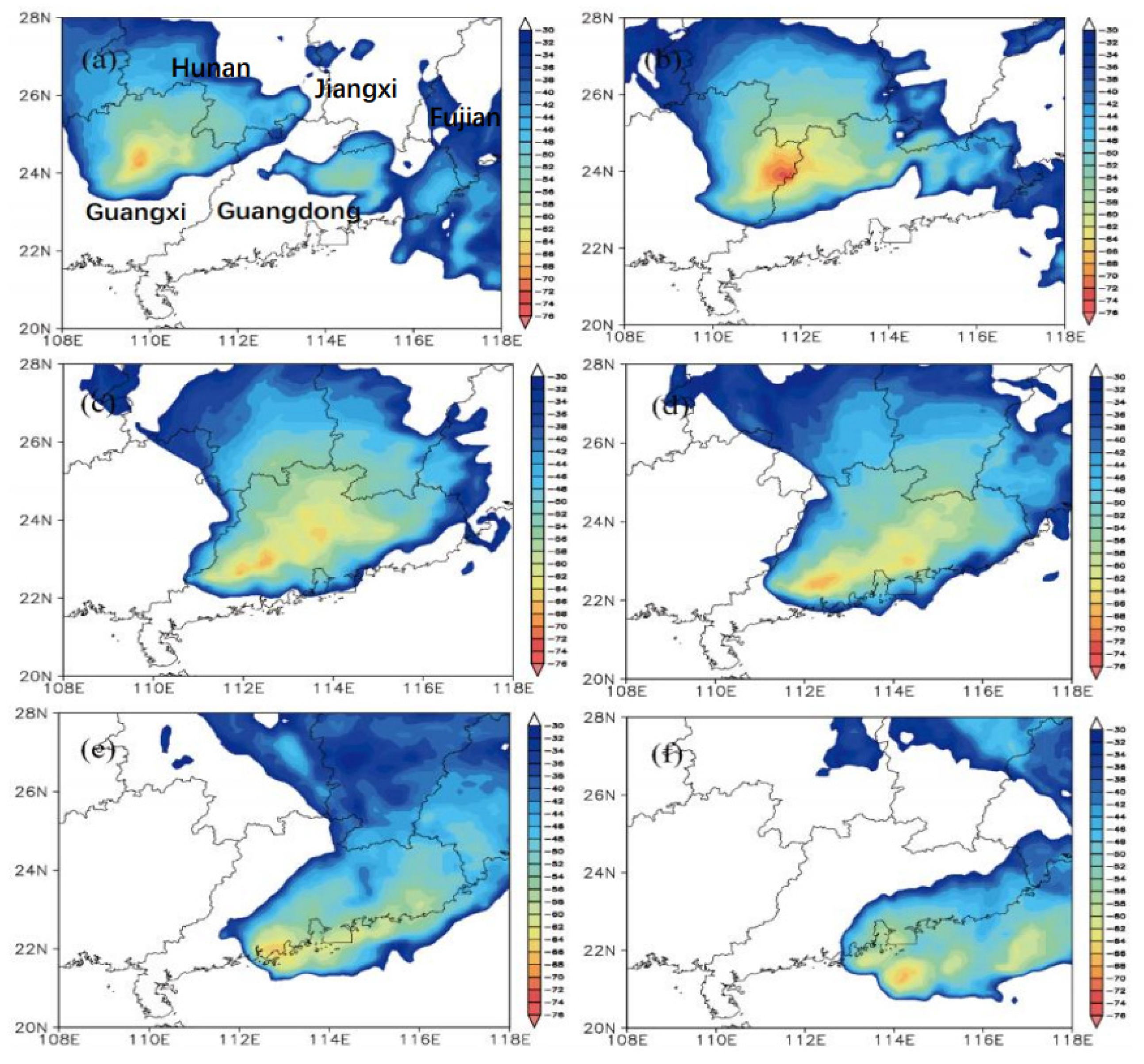
3.1.1. Introduction to the Squall Line Process

During 29–31 March 2014, consecutive days of severe convective weather occurred in south China. In the early morning of 31 March, a long squall line swept across most of Guangdong from northwest to southeast, and the process of the squall line was mainly accompanied by heavy rains and strong winds. During the process of the squall line, the largest quantity of precipitation in the southeast region of Guangdong reached 160 mm/h. On the morning of 31 March, gale weather appeared. Gusts that were equivalent to 12 on the Beaufort scale were detected in some areas, and the maximum gale wind speed was 34.8 m s−1.
The infrared image of the FY-2E geostationary meteorological satellite clearly shows the generation, development and evolution of this strong convective system. Figure 1 is the TBB (black body temperature) distribution of the squall line process obtained from the FY-2E geostationary meteorological satellite. The TBB can represent the cloud top and the intensity of convection. At 19:00 UTC on 30 March (Figure 1a), the squall line system was located in the northern part of Guangxi, showing an oval cloud cluster. At 21:00 UTC (Figure 1b), the system moved to the junction of Guangxi and Guangdong, and the cloud cluster developed and expanded. By 23:00 UTC (Figure 1c), the main body of the squall line had completely moved into Guangdong Province. The mature system was composed of a number of medium γ-scale convective systems, and the range of the tail stratus precipitation area increased. At 00:00 UTC on 31 March (Figure 1d), the area of coldest temperature was located in the southern part of the squall line. At 02:00 UTC (Figure 1e), the convective area began to shrink and the structure deteriorated. By 05:00 UTC (Figure 1f), the main body of the squall line had moved over the ocean, and the convective systems then gradually dispersed. The lowest central temperature of the cloud top was located on the south side of the ocean, and the system slowly decayed.

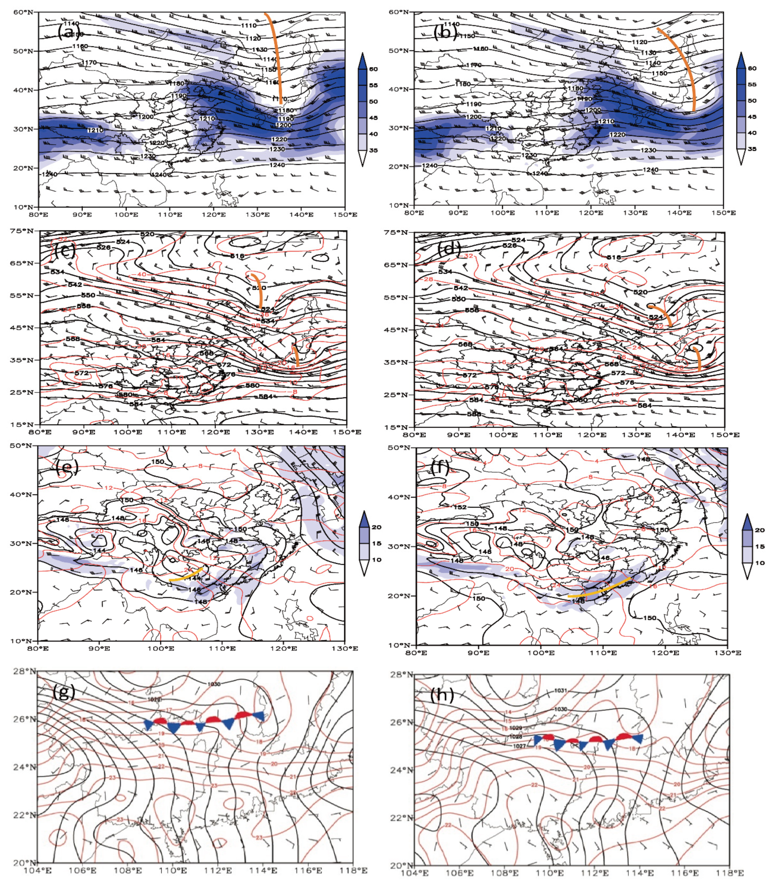
3.1.2. Evolution of Atmospheric Circulation during the Squall Line Process

In contrast to other regions, e.g., the United States, squall lines in South China usually occur in warm and wet areas under monsoon conditions. As South China is located in the low latitudes, the convective systems of squall lines possess weak baroclinic characteristics. The occurrence and development of a squall line in South China is characterized by high temperatures and humidity along with weak baroclinic instability.
Figure 2 represents the Synoptic-scale atmospheric circulation fields of the Meteorological Information Combine Analysis and Process System (MICAPS) data. Figure 2a,b show the 200 hPa geopotential height field and composite wind field at 12:00 and 18:00 UTC on 30 March 2014. The jet stream was located between 20° N and 30° N. At 500 hPa (Figure 2c,d) at the mid–high latitudes, there were two blocking highs (the Ural Mountains and Oktycu Sea), both of which had a tendency to gradually strengthen. The Great Trough of East Asia developed vigorously, and the strong cold air in front of the high-pressure ridge was continuously transported southeastward. In the upper altitudes at low latitudes, there was a south branch trough moving eastwards, and Guangdong was located in the southwestern warm and wet area in front of the trough. At 700 hPa (figure omitted), there were low vortexes moving eastwards, and there was a low airstream flowing southwest in front of the low vortex-trough. There was a shear line in the lower troposphere at 850 hPa (Figure 2e,f), and the low vortexes in the Sichuan Basin moved slowly eastwards under the guidance of the upper-level trough. The low-level jet delivered warm and moist air to the Guangdong and Guangxi area, with the maximum wind speed reaching 16 m s−1. The northern part of Guangxi lay to the left of the low-level jet. To the east of the upper-level trough, the cold air in the northwest was superimposed on the warm and wet air flow at the bottom, which provided favorable conditions for the occurrence of severe convective weather. There was a quasi-stationary front moving southeast at ground level (Figure 2g,h) where warm and cold air was concentrated.
The aforementioned results indicate that this squall line case in South China occurred in the rear of an upper-level trough, to the south of a cold vortex, and at the northwestern edge of the subtropical high. This squall line moved southeastward. The low level airflow at 850 hPa brought abundant water vapor to the region. At ground level, there was a stable quasi-stationary front. This squall line process was closely correlated with the coupling of both lower level and upper level jet streams. This coupled jet not only caused the convergence of strong and cold air and warm and humid air in the South China region, but also formed a large amount of unstable environment and a stable stationary front. Moreover, it also formed a strong vertical wind shear.

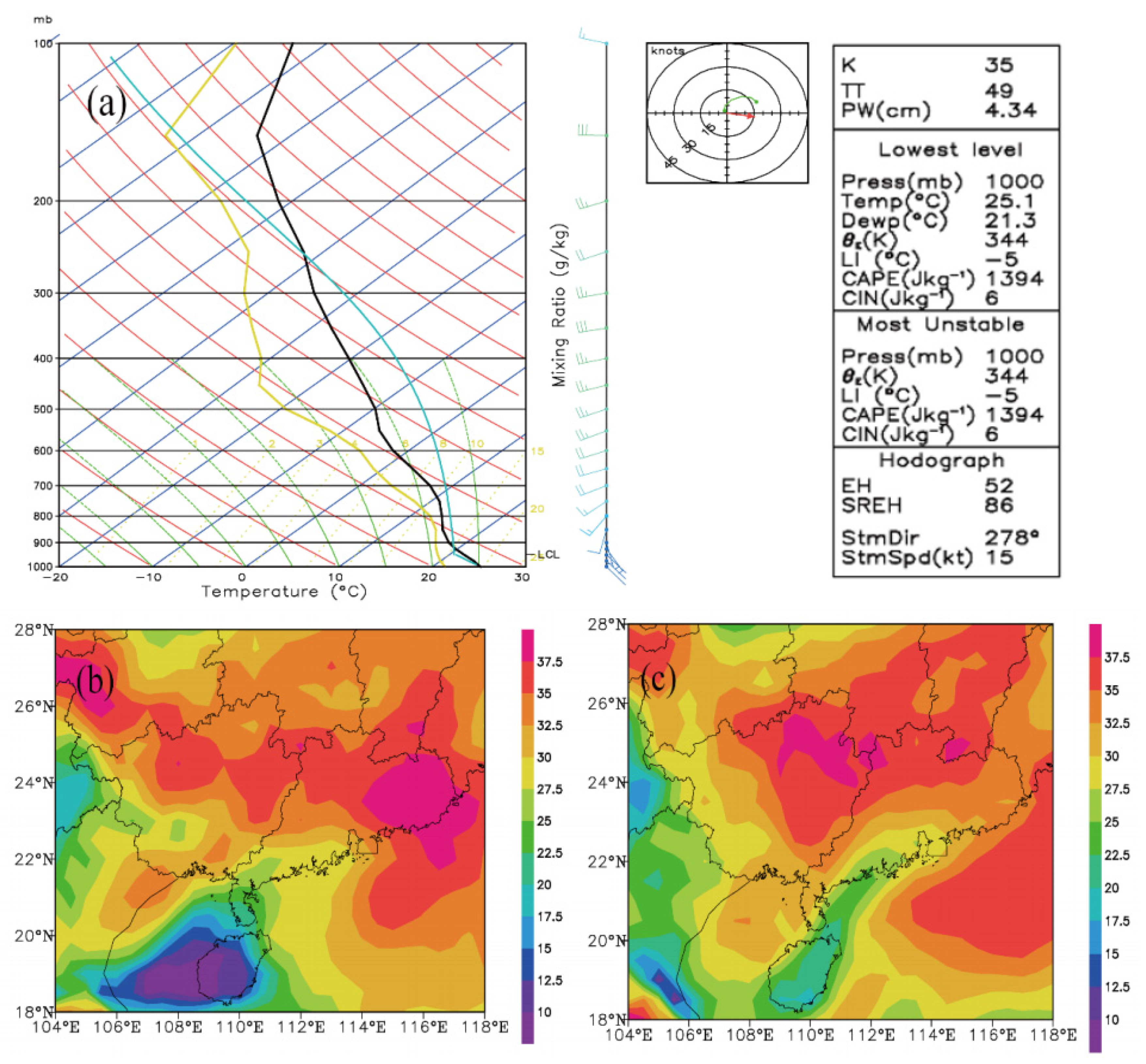
3.1.3. Unstable Stratification

Since the squall line occurred in an area of strong wind shear, which itself was caused by the superp osition of a strong jet and relatively cold air at the top and warm and wet air at the bottom, we produced a regional-mean Skew-T diagram to analyze the atmospheric stratification during the squall line process (Figure 3).
Specifically, Figure 3a shows the simulated atmospheric stratification of the squall line at 12:00 and 18:00 UTC on 30 March 2014. At 00:00 UTC on 30 March, the area-average convective available potential energy (CAPE) was 97.8 J kg−1, while the average convective inhibition (CIN) was 151.2 J kg−1. At 06:00 UTC 30 March, the CAPE increased to 1394 J kg−1 and the average CIN reduced to 6 J kg−1, showing that unstable energy accumulated rapidly in this period of time.
To further study the potential of severe convection, the K index distribution of the simulated area was plotted (Figure 3b,c). It can be seen from the results that the areas of squall line occurrence in South China all had high K index distributions which were above 35 °C. We calculated the K index of the convective region (23°–26° N, 109°–113° E) from 06:00 UTC to 12:00 UTC on 30 March (Figure 3b) and found that the area-average K index was 35 °C. By 18:00 UTC, the K index had risen to 37.5 °C in the region (Figure 3c), showing that the squall line process still had a strong development trend.

3.1.4. Water Vapor Conditions and Vertical Wind Shear

To further reveal the atmospheric environment of the squall line, the water vapor and vertical wind shear field in the simulated area were diagnosed. Figure 4 depicts the vertical wind shear and water vapor flux dispersion fields of 850 hPa at 12:00 UTC and 18:00 UTC on 30 March. In the moisture field (Figure 4b), there were two water vapor transmission channels (from the south and the southwest), and the squall line triggered in northern Guangdong, which was also located at the strong water vapor flux convergence region. At 18:00 UTC, the water vapor flux in South China was significantly enhanced, mainly from the transport of the southeast airflow from the northwestern Pacific Ocean. The strong water vapor convergence center moved to the north of Guangxi and Guangdong, forming a strong water vapor convergence region at the junction of Guangxi and Guangdong.
The squall line occurred under the strong vertical wind shear environment. From the perspective of vertical wind shear at low altitude (Figure 4c,d), southeasterly winds prevailed at 950 hPa at low altitude, with southerly winds at 850 hPa and southwesterly winds at 700 hPa. Also, by 14:00 UTC 30 March, the average vertical low level wind shear, which was about 0–3 km in the convection formation region, had reached 19 m/s. As shown in Figure 4, the maximum vertical wind shear at the junction of Guangdong and Guangxi exceeded 24 m−1 at 12:00 UTC 30 March, and the vertical wind shear of the squall line was greater than 18 m−1. The direction of vertical wind shear was southwesterly. By 18:00 UTC, the maximum center of vertical wind shear had increased to 27 m−1 and moved eastwards to Guangdong Province.

3.2. Design and Testing of the Numerical Simulation

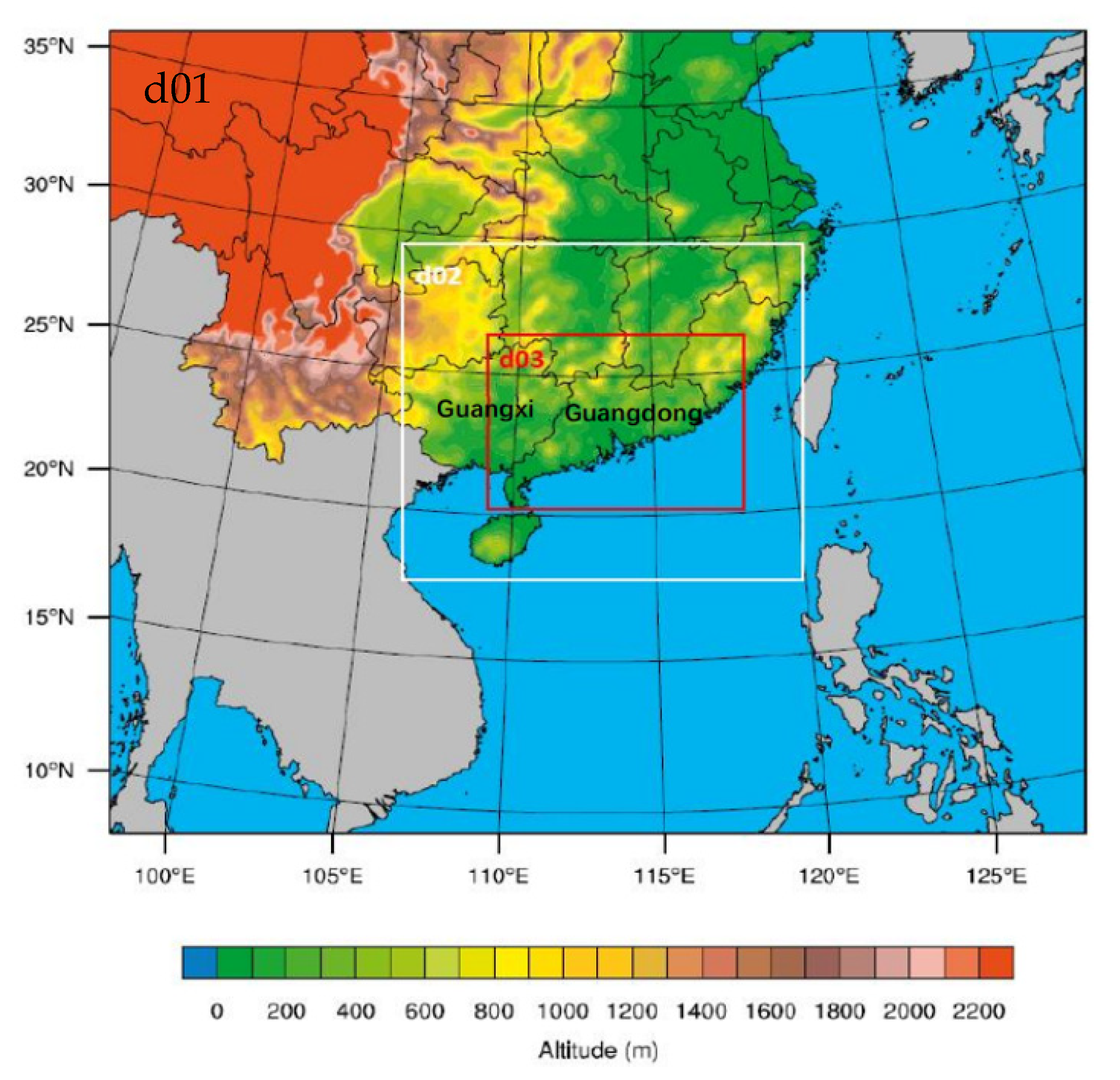
3.2.1. Data and Model Configuration

In order to simulate and reproduce the occurrence and development of the squall line, we used version 3.6 of the WRF model. The specific configuration is shown in Table 1.
The model was designed with three domains and two-way nesting (Figure 5). Each domain has 61 vertical levels with the model top at 50 hPa. The 3-h GFS data was chosen as the initial and boundary condition with the resolution of 0.5 degrees. The first and second grids adopted the cumulus parameterization scheme of the Krain-Fritsch scheme, while the third grid did not use the cumulus parameterization scheme. Dudhia’s radiation scheme and YSU’s planetary boundary scheme were adopted in the three-layer grid. The Morrison scheme was used for the microphysical process with which we had the best simulation compared to other microphysical schemes and the microphysical processes of the Morrison scheme are easier to calculate and analyze. The initial simulation time was 12:00 UTC on 30 March 2014, with 12 h of integration time and about 6 h for spinning-up.

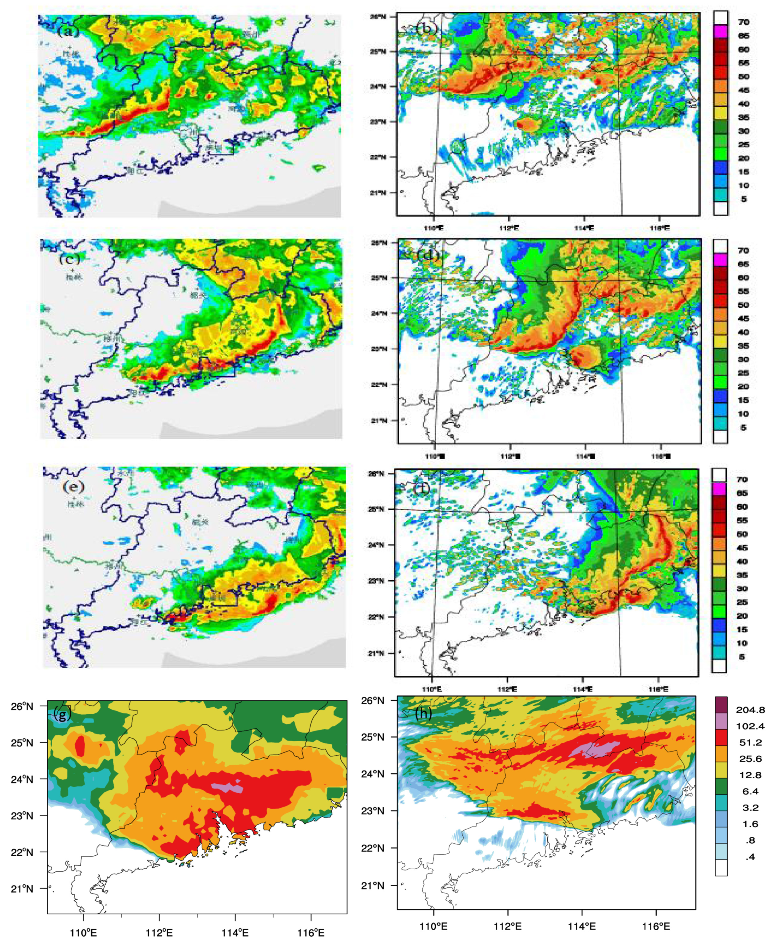
3.2.2. Testing of the Simulation Results

The evolution of the convective activity of the squall line was well simulated by the numerical experiment. Figure 6 compares the observed and simulated radar reflectivities.
Compared with observation, the simulated squall line developed a little later, and slightly to the northwest. At 23:00 UTC 30 March (Figure 6b), the simulated squall line was similar to that at 22:00 UTC 30 March (Figure 6a). There was a lag of about one hour, and the convective system was organized to form the banded structure of the squall line. The observed and simulated lengths of the squall line were similar. The intensity and range of the simulated squall line were consistent with the trend and the actual squall line, enabling the simulation to reflect the life history of the occurrence, development and decline of this squall line case. The numerical experiment also simulated the precipitation processes of the squall line. The maximum value of the simulated accumulated precipitation was relatively close to the actual situation, both of which exceeded 102.4 mm/h, but the area of maximum values and the overall range were slightly north compared with the actual situation.
In general, the simulation was an accurate reproduction of the squall line process based on reflectivity and rainfall compared to the observations. Although there was a certain amount of deviation from the actual situation, it did not affect the analysis of the dynamic and thermodynamic characteristics of the squall line and its microphysical characteristics. We were confident that the simulation results could be used for detailed analysis and diagnosis of this squall line case.

4. Results

4.1. The Dynamic and Thermodynamic Structure and Microphysical Characteristics of the Squall Line

Since this squall line case in South China occurred in the background of the humidity of the East Asian Monsoon and a strong development of the northeast cold vortex, the characteristics of its dynamic, thermodynamic and microphysical structure are unique with respect to their spatial and temporal distribution. In this section, based on the results of a high-resolution numerical simulation, the occurrence and development of the squall line, as well its dynamic, thermodynamic and microphysical structure, are analyzed in detail.

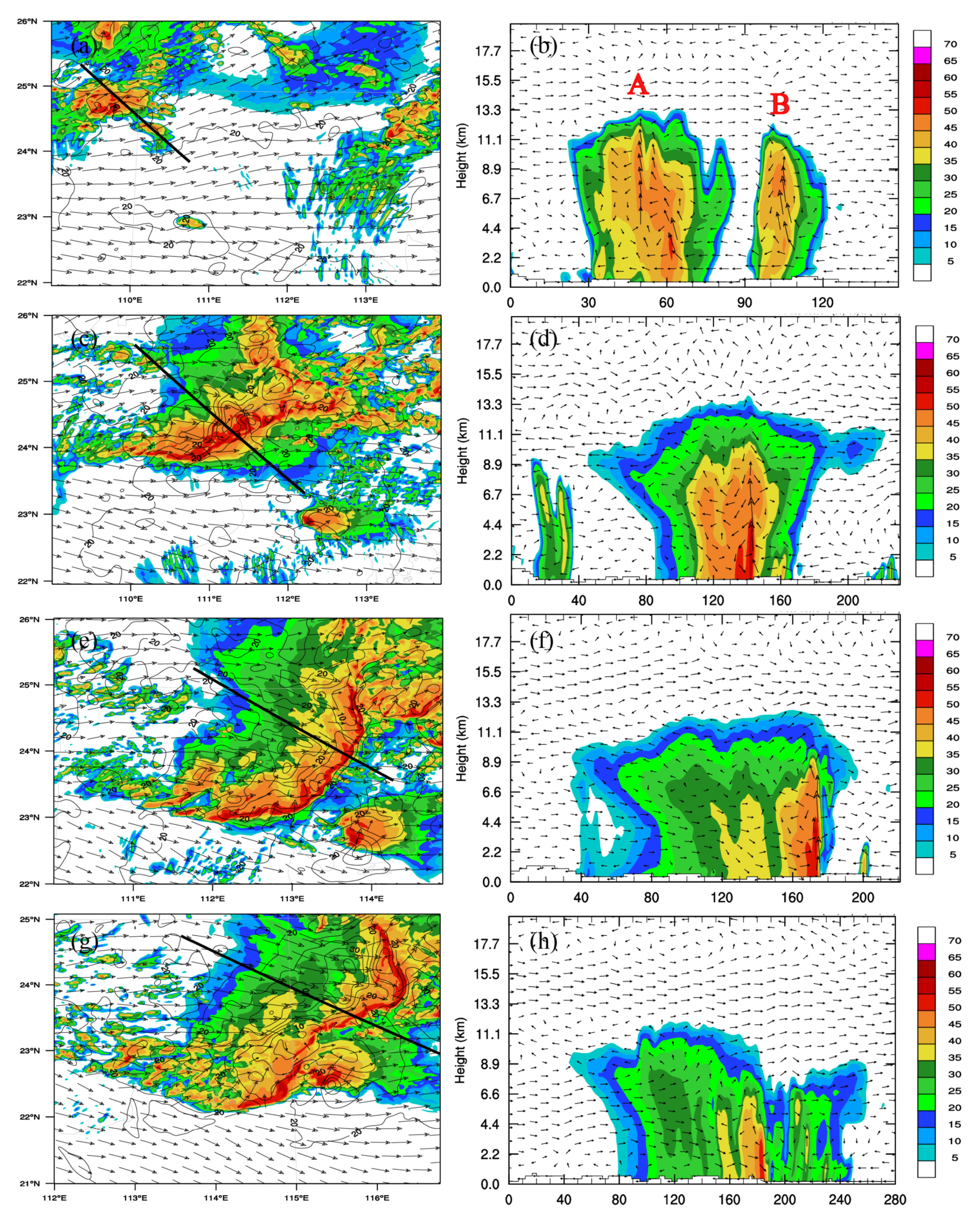
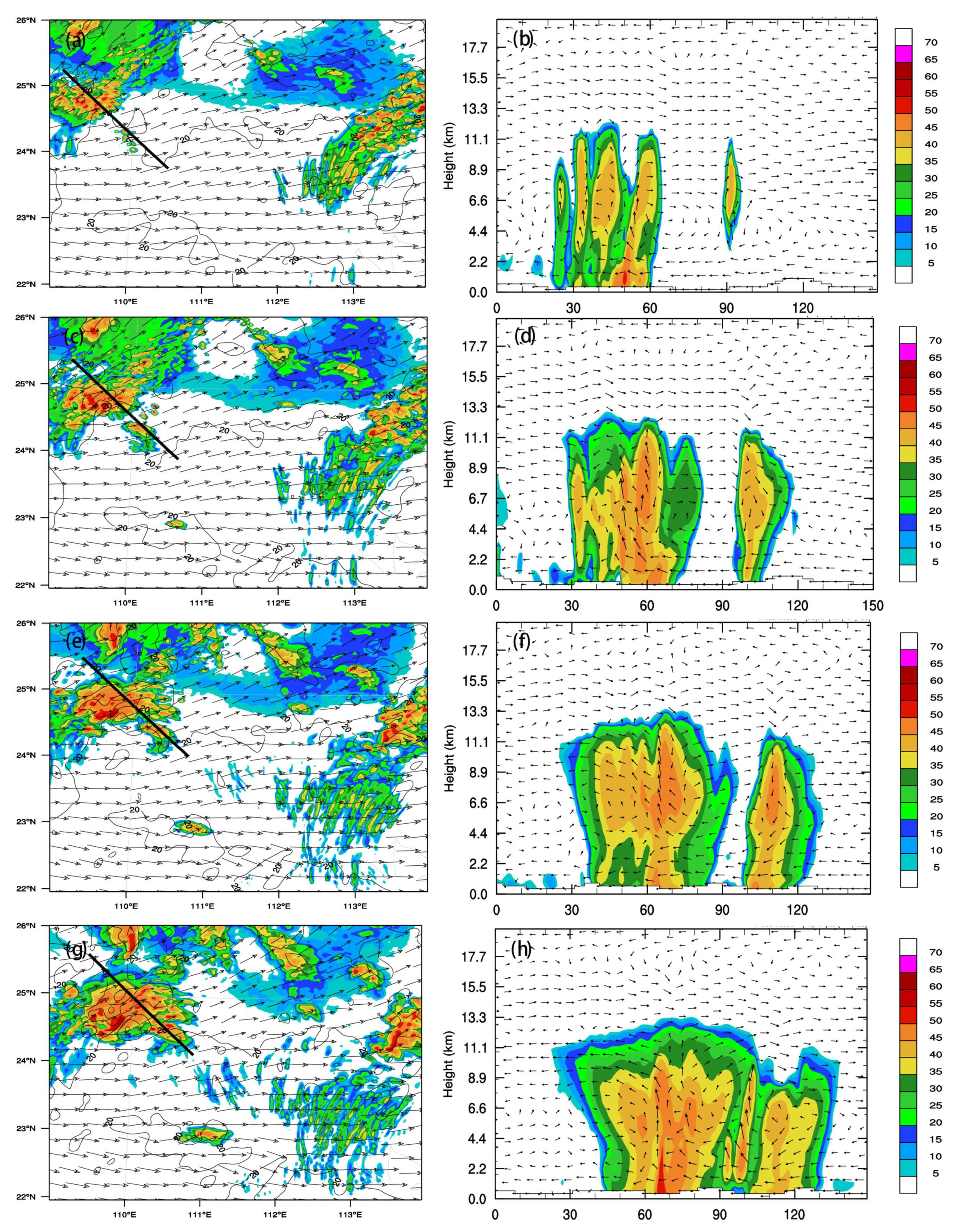
4.1.1. Spatiotemporal Evolution and the Dynamic and Thermodynamic Structure of the Squall Line

In order to study the spatiotemporal evolution and the dynamic and thermodynamic structure of the squall line in different periods, we conducted a comprehensive analysis of the squall line from the aspects of radar reflectivity, rear inflow jet, and vertical movement. The initial period of the squall line, the development period of convection, the maturation period of the system, and the declining period of the system are represented by 20:00 UTC on 30 March, 23:00 UTC on 30 March, 02:00 UTC on 31 March, and 05:00 UTC on 31 March in the simulation (Appendix B Figure A1).
The movement and development of the convective system could be clearly seen from the radar reflectivity. In the initial period (Figure 7a,b) the convective system developed in northern Guangxi. Cells B and A continued to develop and eventually merged into the squall line system. During the developing period of the convective system (Figure 7c,d), the squall line had an obvious linear structure, which had moved to the junction of Guangxi and Guangdong. The horizontal scale of the squall line increased significantly. During the maturation of the system (Figure 7e,f), the entire squall line transferred into Guangdong Province. The system had a typical bow reflectivity structure. At this time the trailing stratiform region increased in size compared with that in the developing period. During the period of decline (Figure 7g,h), the bow structure of the system became fractured, dividing into southern and northern parts, the former of which moved over the ocean surface.
During the cell merging process along the direction of movement in the initial period of the squall line, a vertical circulation system existed between the two cells where there was updraft in cell A and at the upper level the wind blew towards cell B and then sank to the left of monomer B. Influenced by this vertical circulation, the two cells continued to develop and move, with the strong convective system at the rear moving faster than that at the front, until they eventually merged. The linear structure of the combined squall line gradually developed into a strong squall line system. It could be seen that, during the occurrence and development of the squall line, a small vertical circulation between cells B and A, which can be called secondary circulation in the mesoscale environment caused by the development of cells, promoted the organizational development of convective systems. At the same time, the continuous triggering of new cells at the front edge of the squall line affected the development and movement of the squall line to a certain extent.
The dynamic and thermodynamic structures of the squall line in different development periods are shown in Figure 8. In the initial period (Figure 8(a1–a3,b1–b3)), there was an area of ascending motion on the right-hand side of cell A, while there was a center of subsidence on the left-hand side. The right-hand side of cell B also featured a center of ascending motion. The upper and middle layers of the troposphere were flows from cell B to cell A, which corresponded to the vertical circulation mentioned above. During the convective development period (Figure 8(c1–c3,d1–d3)), there was a center of subsidence above the front of the maximum center of ascending motion, and there was a series of subsidence areas behind the ascending motion center and near the ground. From the perspective of the horizontal wind field, there was forward inflow in the front and lower layers of the squall line system, while at the middle and lower layers of the rear part of the system there was elevated downward inflow. During the maturation of the system (Figure 8(b1–b3)), the ascending motion at the convective center within the squall line became further intensified. At the same time, it could be seen that, as the height increased, the ascending motion tended to tilt backwards. The pressure difference between the positive buoyancy in this area and the negative buoyancy in the upper area of the cold pool strengthened the backward-entry flow, forming a positive feedback mechanism. At this time, the lower forward inflow obviously decreased, and the rear inflow jet increased significantly. During the period of decline (Figure 8(c1–c3)), it was clear that the convection inside the system of the squall line was significantly weakened, the forward inflow was obvious, and the rear inflow jet was weakened. Together, these factors meant the system was in a gradual decline.
For the non-adiabatic heating process of the squall line (Figure 8(a3–d3)), a typical three-layer structure could be seen clearly throughout the whole process; specifically, a cooling effect at lower levels, large areas of heating in the middle layers, and a cooling effect again at higher levels. Additionally, it is important to note that the initial phase of cell B’s rise in high-level cooling was more obvious than that of cell A. Furthermore, in the development and maturation stages, the lower-level cooling and middle-level heating centers moved forwards.

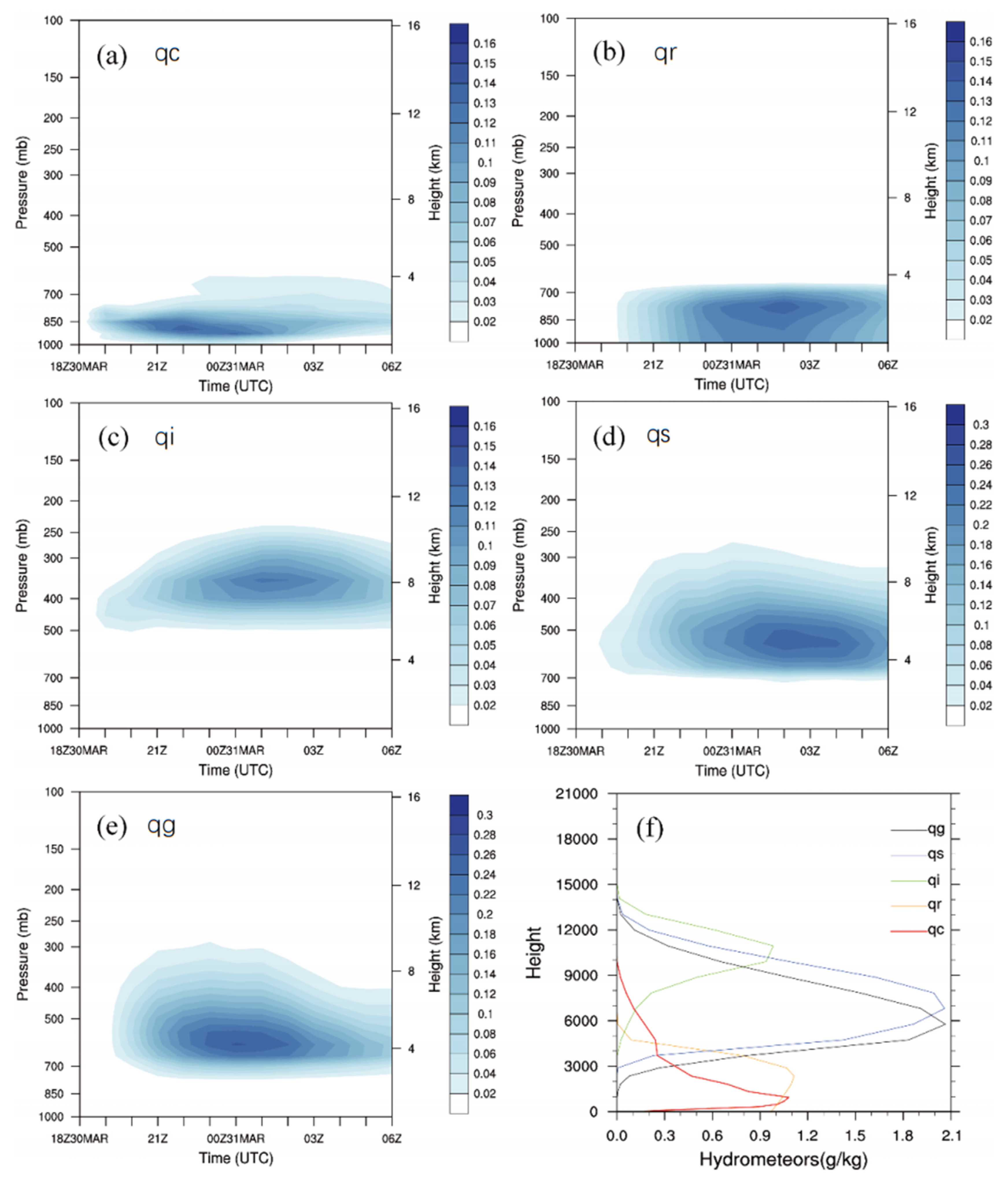
4.1.2. Microphysical Characteristics and Structure of the Squall Line in Different Periods of Development

We analyzed the microphysical characteristics and structure of the squall line from the aspects of the distribution and evolution of the microphysical transformation rate and the latent heat of the phase transformation. The WRF model was used to output the main microphysical processes of water vapor (qv), cloud water (qc), rain water (qr), ice (qi), snow (qs), and graupel (qg), as well as the mixture ratios of the five water condensates and the main microphysical processes of conversion between the five kinds of water condensation.
From the vertical distribution of five kinds of water condensation particles (Figure 9), the system was a typical three-layer cloud structure. That is, the ice crystal particles were concentrated in the upper troposphere. Snow particles and graupel particles were mainly distributed in the middle troposphere. In the lower troposphere, cloud water and rainwater were the most abundant. From the time–height evolution diagram of the water condensation, it could be seen that the five kinds of water condensation first increased and then decreased with time, but the time when the maximum value of each water condensation type occurred was different. The cloud water increased rapidly and reached a maximum at 22:00 UTC 30 March, and then began to decrease after entering the maturation period. Several other water condensation particles reached their maximum during the maturation period.
By comparing the conversion rates of 35 microphysical processes’ output from the model, we selected 20 major microphysical processes for further analysis (Figure 10). The microphysical processes with the highest conversion rates were water vapor condensation into cloud water (PCC+), the collision and growth of cloud water into rain water (PRA), graupel melting into rainwater (PGMLT), cloud water collected by graupel (PSACWG), rainwater collected by snow (PRACS), rainwater collected by graupel (PRACG), and evaporated rainwater (PRE).
The process of water vapor condensation into cloud water (PCC+) was dominant in the four periods, and was distributed from the lower layer to the upper layer of the troposphere. In the initial period (Figure 10a), water vapor condensation into cloud water had the largest conversion rate. The process of cloud water hitting and growing into rainwater (PRA) was relatively concentrated in the middle and lower layers of the troposphere, meaning there was always a large amount of supercooled cloud water in the upper troposphere. The vaporization of supercooled cloud water (PCC-) promoted the Bergeron process in the cold cloud. After entering the development period, graupel melting into rainwater (PGMLT) had the highest conversion rate, and continued during the decline of the process, which made an important contribution to the production of rainfall.

4.2. Possible Mechanism of Development and Evolution of the Squall Line

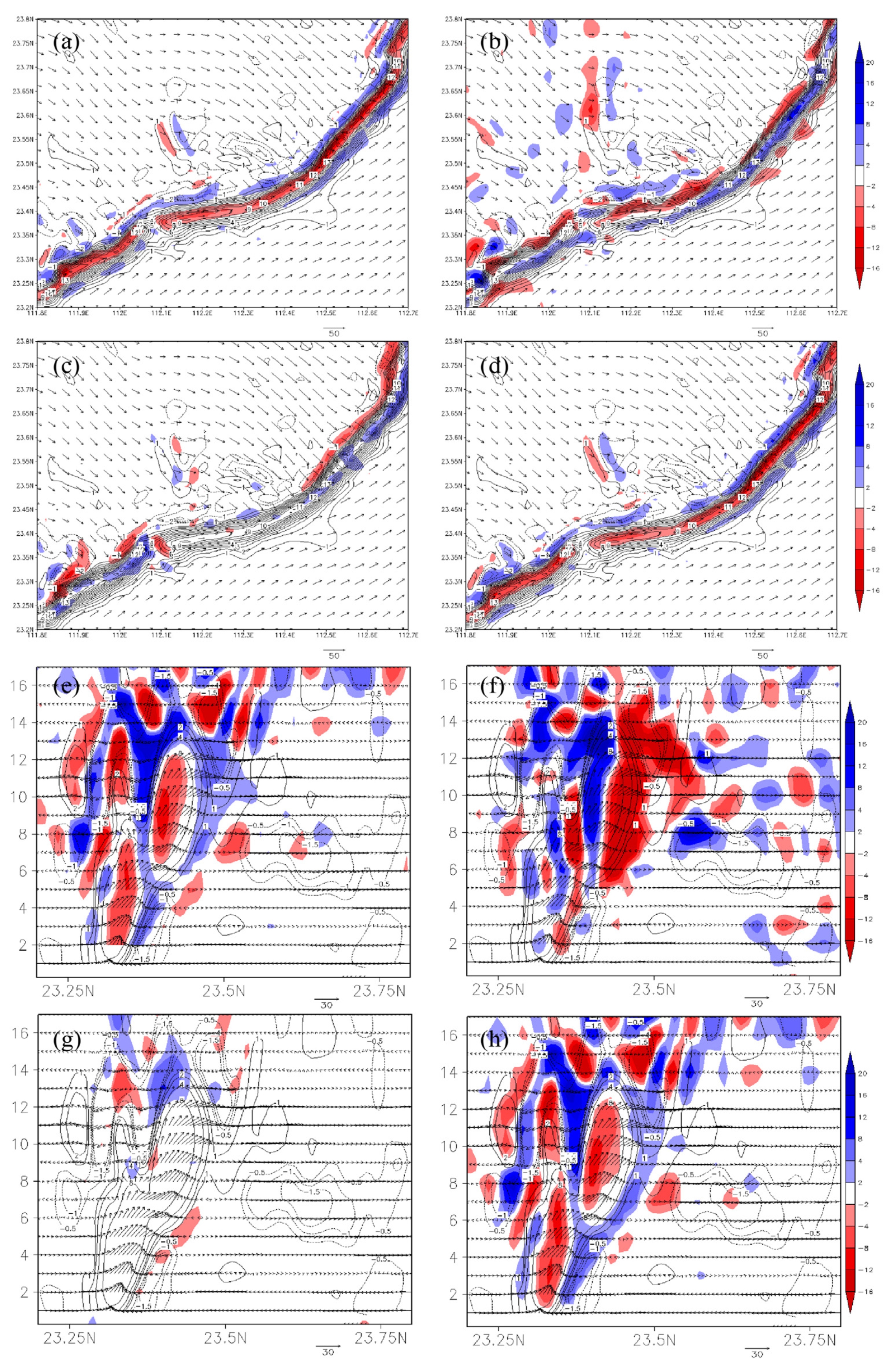
4.2.1. Introduction and Analysis of Complete Q Vectors

In this study, we diagnosed the forcing of each term on vertical motion.
We selected the maturation stage of the squall line at 02:00 UTC 31 March as the target to draw the Q vector and its various diagrams. As shown in Figure 11a, the convergence region of the Q vector corresponded to ascending motion, while the divergence region corresponded to descending motion. Figure 11b shows the quasi-vorticity term. The divergence region corresponded to ascending motion, while the convergence region corresponded to descending motion, demonstrating that the quasi-vorticity term played a negative role in the development of the squall line. However, its magnitude was 10 15 , which, compared with the other two terms, was relatively small, meaning its impact on the Q-vector relative to the other factors was insignificant.
Figure 11c shows the frontogenesis term. The divergence region corresponded to ascending motion, while the convergence region corresponded to descending motion. From the section the magnitude was smaller, so the effect was comparatively small.
Figure 11d shows the non-adiabatic term. The convergence region corresponded to ascending motion, while the divergence region corresponded to descending motion, which made a positive contribution to the development of the squall line. Its magnitude was equivalent to the total Q vector, and its shape was closer to that shown in Figure 11a, which was the main term for the Q vector. Therefore, during the process of occurrence and development of the squall line, the adiabatic force played the main role, rather than the dynamic force.
Figure 11e–h shows that the convergence region of the Q vector almost corresponded to ascending motion at all levels. In general, the Q vector played a positive role in the development of the squall line and showed the importance of the adiabatic force.

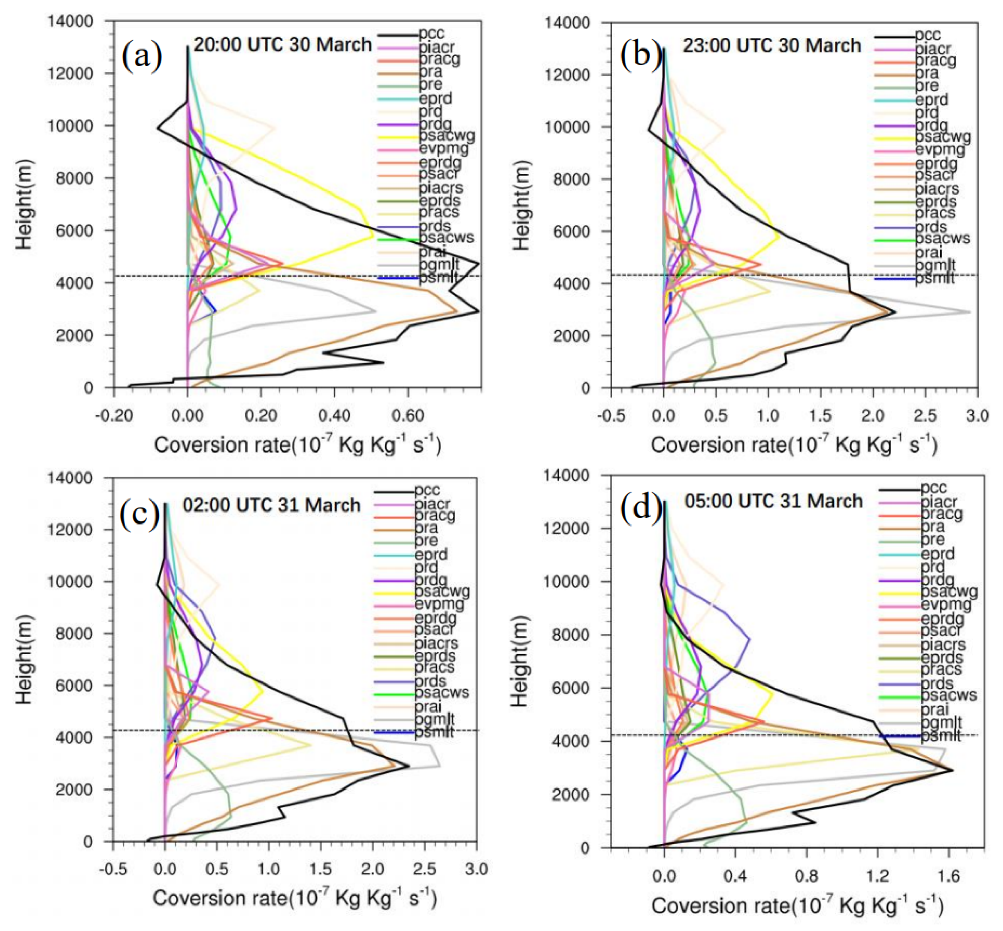
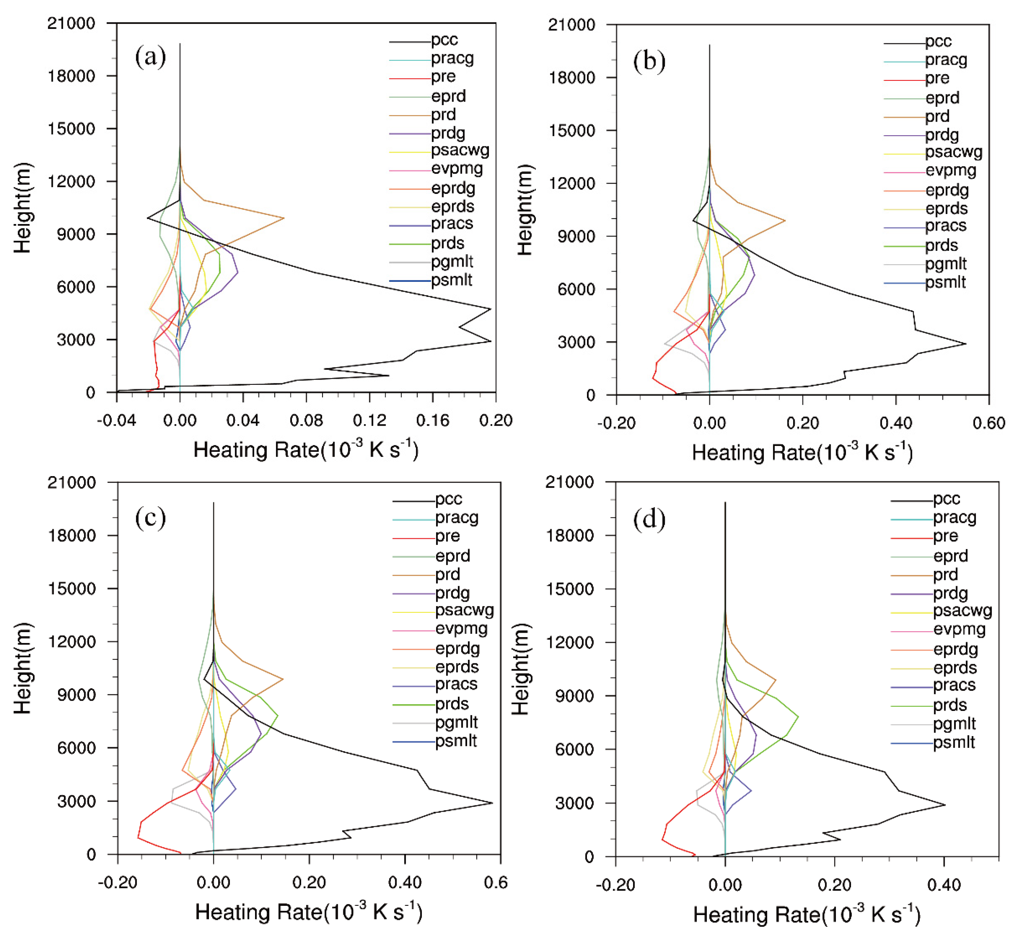
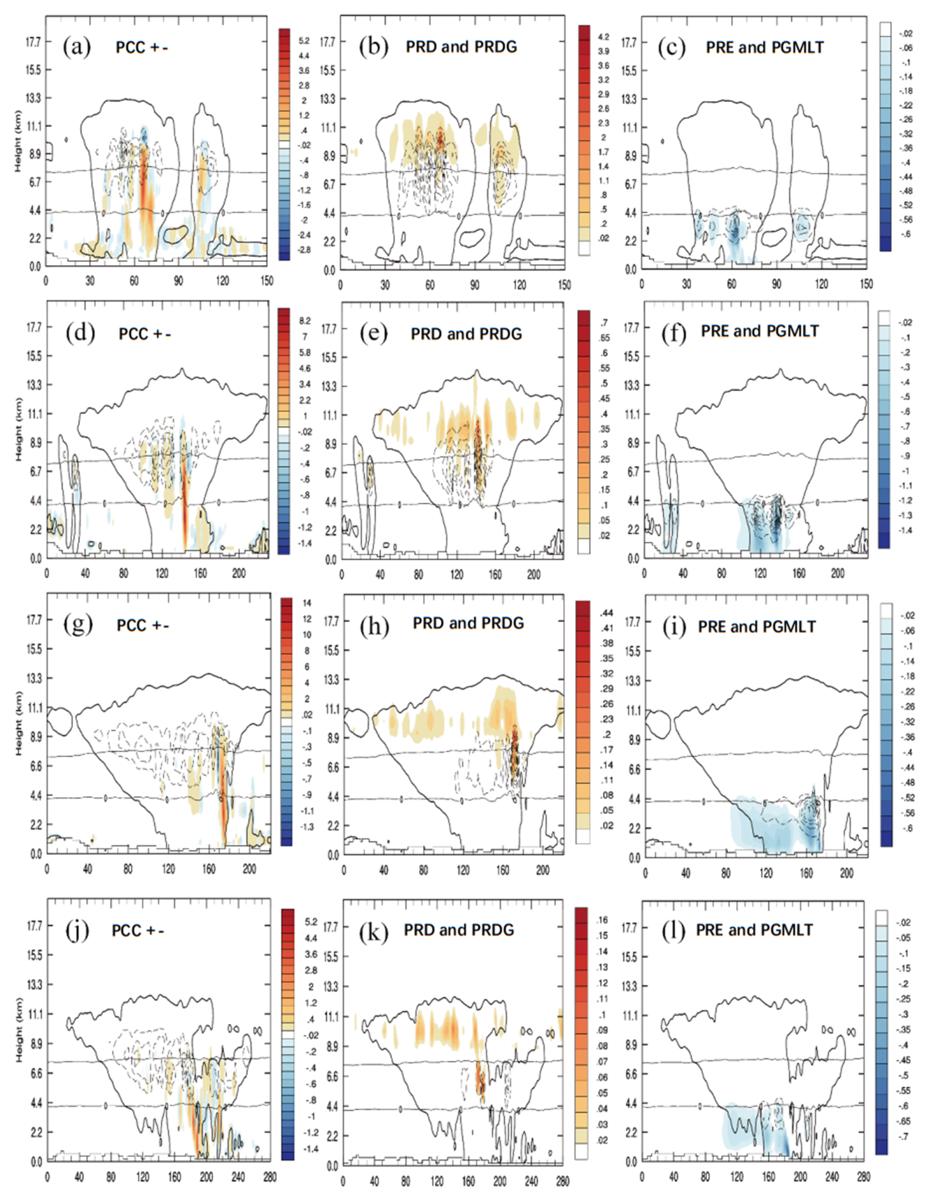
4.2.2. Microphysical Heat Budget during the Development of the Squall Line

The phase-change latent heat of microphysical particles can heat and cool the air, thus affecting the dynamic and thermodynamic processes of a squall line. Heating processes typically involve freezing and condensation, which releases latent heat during the phase transformation and leads to atmospheric heating. These cooling processes mainly include evaporation, melting and sublimation. These cooling processes absorb latent heat during phase transformation processes that cool the atmosphere. According to the output results of the model, we used the methods developed by Hjelmfelt et al. (1989) [30] to calculate the rates of non-adiabatic heating, cooling, and their net rate of change, according to the following formula (14 microphysical processes with relatively large contribution rates were selected):
R w = ( L v C p ) × ( pcc ( + ) ) + ( L f C p ) × ( pracg + pracs + psacwg ) + ( L s C p ) × ( prdg + prds + prd ) ,
R c = ( L v C p ) × ( pcc ( ) + pre + evpmg ) + ( L f C p ) × ( pgmlt + psmlt ) + ( L s C p ) × ( eprdg + eprds + eprd ) ,
R t = R w + R c
Here, L v is the latent heat constant of evaporation; L f is the latent heat constant of melting; L s is the latent heat constant of sublimation (units: J kg−1); C p is the specific heat capacity of moist air at reference temperature (units: J kg−1 K−1); pxxxx and exxxx are the conversion rates of microphysical processes (units: kg kg−1 s−1); and R w , R c and R t are the total rates of heating, cooling and net heating, respectively.
Figure 12 shows the vertical distribution of the phase-change latent heat rate of 14 microphysical processes, which made major contributions, over four periods. During the whole process, the heat source was mainly water vapor condensing into cloud water (PCC+), water vapor condensing into ice crystals (PRD), water vapor condensing into graupel (PRDG), and water vapor deposition into snow (PRGS). The cold source was mainly the evaporation of cloud water near the ground (PCC−), the evaporation of rainwater at the lower layer (pre), the melting of graupel into rainwater (PGMLT), the sublimation of graupel into water vapor (EPRDG), and the sublimation of snow into water vapor (EPRDS). Among them, the evaporation of rainwater (PRE) at the lower layer was the most significant. All abbreviations can be found in the Appendix A Table A1.
Through the above analysis, we gained a certain understanding of the distribution of the rate of phase change in latent heat in the squall line system in terms of time and height. Below, we further analyze the distributional and evolutionary characteristics of the squall line system by using a vertical section of the rate of phase change in latent heat of several microphysical processes that contributed markedly.
As can be seen from Figure 13, the maximum heating rate and the maximum cooling rate of the microphysical processes both appeared in the stratiform region within the system. Water vapor condensation to cloud water (PCC+) and the evaporation of cloud water (PCC−) extended from the bottom layer to the middle and high layer to 9 km. The maximum heating rate of water vapor condensing into cloud water (PCC+) corresponded to the strong updraft area. The deposition of water vapor into ice crystals (PRD) was concentrated near the upper troposphere at 10.5 km. The maximum cooling rate of rainwater evaporation (PRE), which was the main cooling process, was concentrated in the middle and lower troposphere, corresponding to the strong downdraft at the lower layer (Figure 13b).
During the maturation of the system (Figure 13g–i), the heating rate of water vapor condensing into cloud water (PCC+) continued to increase, and the heating range of water vapor condensing into snow (PRDS) increased with the expansion of the system’s cloud area, and the intensity also increased. The heating strength of the deposition of water vapor into ice crystals (PRD) and graupel (PRDG) was weakened. The range of low-level rainwater evaporation (PRE) cooling was further expanded, which corresponded to the range of cold pools in this period. The evaporation of rainwater (PRE) made an important contribution to the surface cold pools. Compared with the previous period, it could clearly be seen that the melting of graupel into rainwater (PGMLT) was consistent with the distribution of the rear inflow jet of the squall line, and the melting and cooling of graupel particles in the dry and cold air brought by the rear inflow jet also made an important contribution to the surface cold pool.
During the decay period (Figure 13j–l), the heating and cooling rates of each process decreased. The heating of water vapor condensing into snow (PRDS) was still dominant in the upper and middle layer of the convective system, so the content of snow particles was the most important. The heating rate of water vapor condensation into snow (PRDS) was slightly smaller than that of other heating processes, but it played an important role in the growth of stratus cloud.

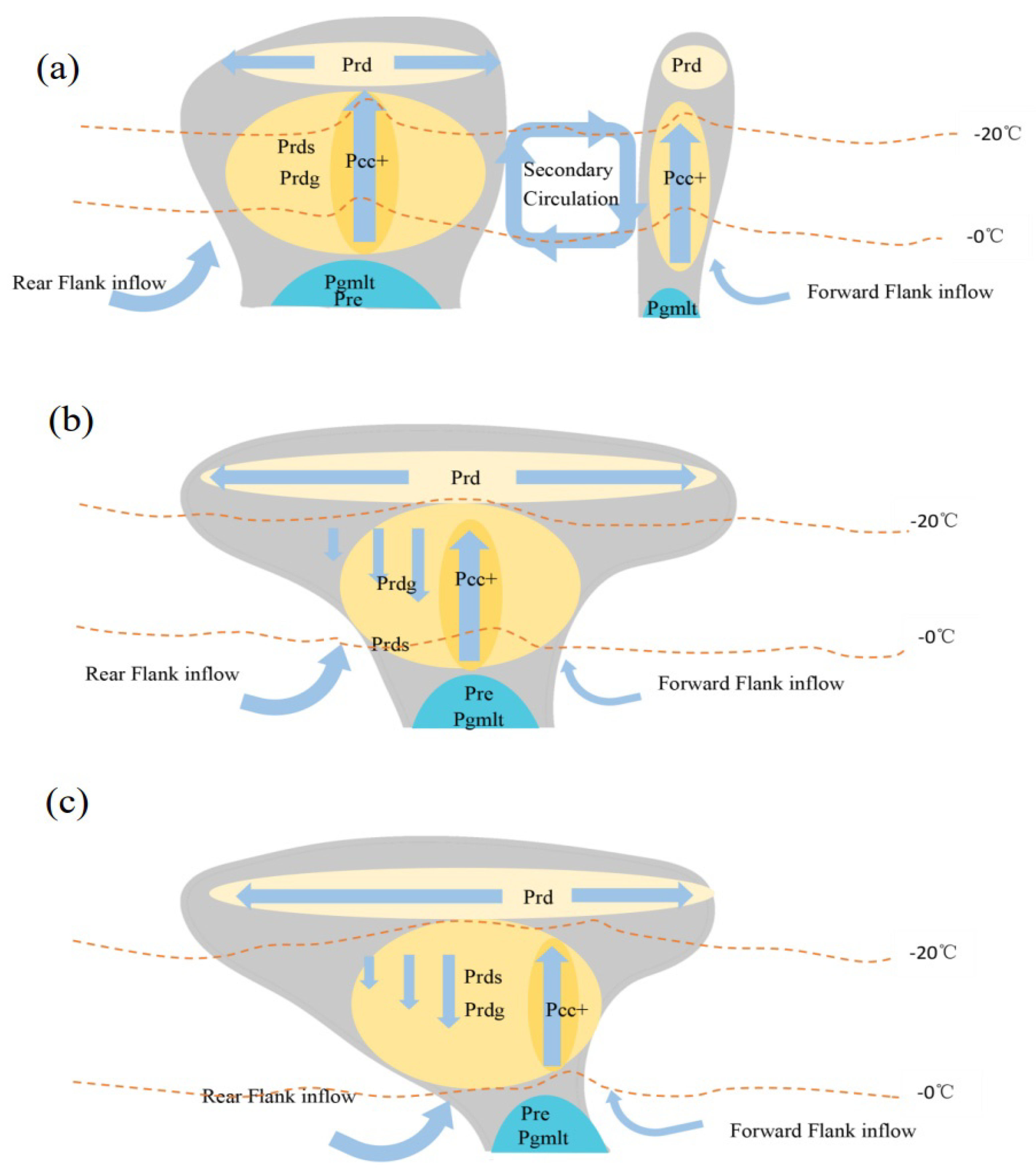
4.2.3. Possible Mechanism of the Squall Line’s Development and Evolution

The formation and extinction mechanism of the squall line was summarized by dynamic and thermodynamic analysis and cloud microphysical analysis (Figure 14).
During the development of the squall line, along with the merging of cells along the direction of movement, there was a vertical circulation system between the two cells. Under the influence of this vertical circulation, the two cells kept developing and moving. From the perspective of microphysical processes, the centers of the two cells’ ascending motion were supported by the PCC + process. The forward inflow of the ground-level branch, moving over the cold pool area of cell A, formed into a strong ascending inflow with the forward inflow of cell B. Cell B was thriving, so the effect of upper-air divergence was stronger; when its air flow extended to the rear of cell A, it began to decline, which formed an obvious secondary circulation system in the course of the two cells. The two cells came closer under the influence of compensation drag in this secondary circulation, eventually merging with the squall line system. During the process of the occurrence and development of the squall line, the development of mesoscale vertical secondary circulation promoted the organizational development of the merging of convective systems. At the same time, the development and movement of the squall line was affected to a certain extent by the continuous triggering of new cells at the front edge of the squall line.
The analysis of the mesoscale Q vector showed that the effect of non-adiabatic heating was stronger than that of dynamic forcing. Rainwater evaporative cooling had good corresponding relationships with strong subsidence movement within the system and the scope of the cold pool. The process of rainwater evaporation made an important contribution to the ground-level cold pool, and cold pools triggering convection was one of the important processes of this squall line case.
The rear inflow jet also played an important role in the enhancement of the squall line system. The melting of graupel into rainwater corresponded well with the rear inflow jet. Therefore, the rear inflow jet mainly brought cold air formed by the melting of graupel particles. The rear inflow jet was strongest in the maturation period. At the same time, the squall line system had a strong outflow center in the front and rear of the upper troposphere, forming a strong high-level divergence which was conducive to the low-level inflow and the ascending motion of strong convection, thus strengthening the development and maintenance of the system. Both the convective region and the stratus cloud region were distributed with a large-value center of rear inflow jet. The strong backflow center in the stratum cloud area cut off the forward inflow from the middle and lower layers to the upper layers in the period of decline. At the same time, the cold pool cut off the transportation of the warm and moist air from the lower layers towards the high layers, which was the cause of the gradual decline of the squall line process.
After the squall line continued to develop into the maturation period, there were evident changes in the internal dynamic and thermodynamic structures. During the maturation period, the vertical rising branch of the squall line moved forwards to the forefront of the squall line, along with the heating area of PCC+ also moving forward. The cold pool moved forward, influenced by the Pgmlt and Pre processes. The cloud tops tilted back, with the inflow becoming the strongest. The inclined structure could be seen clearly and, meanwhile, the development of the squall line was at its most exuberant.
During the period of decline and death of the system, the enhanced rainwater evaporation(Pre) caused the cold pool to be strong enough to move quickly to the front of the storm and block the warm air that supplied the rising movement, leading to the storm’s recession.

5. Discussion and Conclusions

On 31 March 2014, a strong squall line occurred in the southeast of China. The squall line was accompanied by heavy rain and strong winds. In this paper, GFS reanalysis data, satellite data, MICAPS data, and the CMORPH precipitation products were used to analyze the formation and evolution of the squall line. The mesoscale numerical model, WRF, was used to simulate and reproduce the squall line process. The dynamic, thermodynamic and microphysical characteristics of the squall line in different periods were analyzed using the high temporal resolution results of the WRF model. We discussed the change and influence of the cloud microphysical process during the development of the squall line, and the Q vector was used to analyze the non-adiabatic forcing and dynamic forcing of the squall line.
The following conclusions were obtained:
1. A vertical circulation system existed continuously during the merging of convective systems along the direction of movement in the initial period. Under the action of this vertical circulation, the two cells continuously developed and moved, eventually merging into a squall line system.
2. In the maturation period, the rear inflow jet reached its strongest point and, at the same time, there was a strong outflow center before and behind the squall line in the troposphere. This formed a strong divergence of the high layer, thus strengthening the development and maintenance of the system.
3. The strong rear inflow jet center in the stratiform region cut off the forward flow of the middle and low layers towards the high layers during the period when the system declined and eventually died. Combined with the cold pool, this cut off the low-level warm and wet air, which was the cause of the gradual decline of the squall line process.
4. Analysis of the mesoscale Q vector showed that, during the process of the squall line, the non-adiabatic forcing was the main function, rather than the dynamic forcing.
5. Microphysical processes had an important influence on the dynamic and thermodynamic structure of the squall line. The condensation of water vapor to the cloud water (PCC+) provided heat for the ascending motion inside the squall line. The evaporation and cooling of rainwater generated the strengthening of the internal descending motion of the system and the increase in the scope of the cold pool. In addition, there was good correspondence between the melting of graupel into rain and the backflow. The interaction between the inflow and cold pool played an important role in the squall line.
Although the dynamic and thermodynamic characteristics of the squall line and its microphysical characteristics were analyzed in detail, some aspects of the squall line process still need to be studied and discussed further. We only discussed one particular scheme of microphysical processes. This may be only one possible mechanism based on this particular model setting and this particular case. The occurrence and development of the squall line was affected by the interaction of various dynamic, thermodynamic and microphysical processes. In the next stage of this work, we intend to further analyze the different microphysical processes in the squall line. More sensitivity experiments of the microphysical processes are needed, as well as comparison of satellite observation data and simulation. The conclusions of this paper also need to be confirmed through analysis of more squall line cases.
The conclusions of this paper are related to a single squall line process only. In the future, more squall line processes in South China will be studied and verified in order to obtain more broadly representative results. Observation of the detailed microphysical processes that affect squall line systems still need further attention. For instance, the phases, concentrations and droplet distributions of hydrometeors should be retrieved jointly by dual polarization radar, Doppler radar and cloud radar. In addition, further numerical evidence of the microphysical processes and how they affect the development of squall lines needs to be gathered, examined and confirmed.

Author Contributions

Conceptualization, J.L. and F.P.; methodology, J.L. and F.P.; software, J.L. and Y.S.; validation, J.L. and Y.S.; formal analysis, J.L. and Y.S.; investigation, J.L. and Y.S.; resources, F.P.; data curation, F.P. and Y.S.; data curation, Y.S. and J.T.; Writing—original draft, J.L. and Y.S.; writing—review and editing, J.L. and J.T.; visualization, J.L., Y.S. and J.T.; supervision, F.P. and J.T. All authors have read and agreed to the published version of the manuscript.

Funding

This research was funded by the National Basic Research Program of China (Grant number 2018YFC1506801 and XDA17010105), Science and technology Winter Olympics Program (Grant number 19975414D) and the National Natural Science Foundation of China (Grant number 41675059, 41405059, 41375066, U1333130, and 41530427). Simulations were carried out at the National Supercomputer Center in Tianjin on the TianHe cluster.

Institutional Review Board Statement

Not applicable.

Informed Consent Statement

Not applicable.

Data Availability Statement

The data that support the findings of this study are available from the corresponding author upon reasonable request.

Conflicts of Interest

The authors declare no conflict of interest.

Appendix A

Table A1. Description of Microphysical Processes in the Morrison Scheme.
AbbreviationMicrophysical Processes of Morrison SchemeFromTo
evpmsMelting and evaporation of QSqsqv
evpmgMelting and evaporation of QGqgqv
eprdSublimation of Qqiqv
eprdsSublimation of QSqsqv
eprdgSublimation of QGqgqv
piacrCollection QR by QI, conversion to QGqrqg
piacrsCollision QR by QI, conversion to QSqrqs
pracsCollection QS by QRqrqs
pracgCollection QR by QGqrqg
praAccretion QC by QRqcqr
preEvaporation of QRqrqv
prdDeposition of QIqvqi
prdsDeposition of QSqvqs
prdgDeposition of QGqvqg
praiAutoconversion of QIqiqs
psacwsAccretion QC by QSqcqs
psacwgCollection QC by QGqcqg
psmltMelting of QSqsqr
pgmltMelting of QGqgqr
pccCondensation of QV/Evaporation of QCqv/qcqc/qv

Appendix B

Figure A1. Radar reflectivity (units: dBZ) and the vertical wind shear (isolines; interval: 5 m s−1) of 0–3 km (a,c,e,g), along with the vertical profile of radar reflectivity along the sectional line (thick black line) (b,d,f,h), at 20:00 UTC 30 March 2014 (a,b), 21:00 UTC 30 March 2014 (c,d), 22:00 UTC 30 March 2014 (e,f), and 23:00 UTC 310March (g,h). Vectors represent wind speed at 850 hPa.
Atmosphere 12 01187 g0a1

References

  1. Meng, Z.; Yan, D.; Zhang, Y. General Features of Squall Lines in East China. Mon. Weather Rev. 2013, 141, 1629–1647. [Google Scholar] [CrossRef]
  2. Bluestein, H.B.; Jain, M.H. Formation of mesoscale lines of precipitation: Severe squall lines in Oklahoma during the spring. J. Atmos. Sci. 1985, 42, 1711–1732. [Google Scholar] [CrossRef]
  3. Paker, M.D.; Johnson, R.H. Organizational modes of midlatitude mesoscale convective systems. Mon. Weather Rev. 2000, 128, 3413–3436. [Google Scholar] [CrossRef]
  4. Fujita, T.T. Results of detailed synoptic studies of squall lines. Tellus 1955, 4, 405–436. [Google Scholar]
  5. Johnson, R.H.; Hamilton, P.J. The Relationship of Surface Pressure Features to the Precipitation and Airflow Structure of an Intense Midlatitude Squall Line. Mon. Weather Rev. 1988, 116, 1444–1473. [Google Scholar] [CrossRef] [Green Version]
  6. Takemi, T. A sensitivity of squall line intensity to environmental static stability under various shear and moisture conditions. Atmos. Res. 2007, 84, 374–389. [Google Scholar] [CrossRef]
  7. Rotunno, R.; Klemp, J.B.; Weisman, M.L. A theory for strong, long-lived squall lines. J. Atmos. Sci. 1988, 45, 463–485. [Google Scholar] [CrossRef] [Green Version]
  8. Wakimoto, R. The Life Cycle of Thunderstorm Gust Fronts as Viewed with Doppler Radar and Rawinsonde Data. Mon. Weather Rev. 1982, 110, 1060–1082. [Google Scholar] [CrossRef] [Green Version]
  9. Engerer, N.A.; Stensrud, D.J.; Coniglio, M.C. Surface Characteristics of Observed Cold Pools. Mon. Weather Rev. 2008, 136, 4839–4849. [Google Scholar] [CrossRef]
  10. Zhang, L.; Sun, J.; Ying, Z.; Xiao, X. Initiation and Development of a Squall Line Crossing Hangzhou Bay. J. Geophys. Res. Atmos. 2021, 126. [Google Scholar] [CrossRef]
  11. Fujita, T. Precipitation and cold air production in mesoscale thunderstorm systems. J. Meteorol. 1959, 16, 454–466. [Google Scholar] [CrossRef] [Green Version]
  12. Biggerstaff, M.I.; Houze, R.A. Kinematic and Precipitation Structure of the 10–11 June 1985 Squall Line. Mon. Weather Rev. 1991, 119, 3034–3065. [Google Scholar] [CrossRef]
  13. Braun, S.A.; Houze, R.A. The Transition Zone and Secondary Maximum of Radar Reflectivity behind a Midlatitude Squall Line: Results Retrieved from Doppler Radar Data. J. Atmos. Sci. 1994, 51, 2733–2755. [Google Scholar] [CrossRef] [Green Version]
  14. Braun, S.A.; Houze, R.A. The Evolution of the 10–11 June 1985 PRE-STORM Squall Line: Initiation, Development of Rear Inflow, and Dissipation. Mon. Weather Rev. 1997, 125, 478–504. [Google Scholar] [CrossRef]
  15. Leary, C.A.; Houze, R.A. The Structure and Evolution of Convection in a Tropical Cloud Cluster. J. Atmos. Sci. 1979, 36, 437–457. [Google Scholar] [CrossRef] [Green Version]
  16. Lord, S.J.; Willoughby, H.E.; Piotrowicz, J.M. Role of a Parameterized Ice-Phase Microphysics in an Axisymmetric, Nonhydrostatic Tropical Cyclone Model. J. Atmos. Sci. 1984, 41, 2836–2848. [Google Scholar] [CrossRef] [Green Version]
  17. Guo, X.L.; Fu, D. Formation process and cloud physical characteristics of a typical disastrous hailstorm and gale in Beijing. Atmos. Sci. 2003, 27, 618–627 (In Chinese). (In Chinese) [Google Scholar]
  18. Adams-Selin, R.D.; Heever, S.C.V.D.; Johnson, R.H. Sensitivity of Bow-Echo Simulation to Microphysical Parameterizations. Weather 2013, 28, 1188–1209. [Google Scholar] [CrossRef]
  19. Szeto, K.K.; Cho, H.R. A numerical investigation of squall lines. Part II: The mechanics of evolution. J. Atmos. Sci. 1994, 51, 425–433. [Google Scholar]
  20. Van Weverberg, K.; van Lipzig, N.P.; Delobbe, L. The impact of size distribution assumptions in a bulk one-moment microphysics scheme on simulated surface precipitation and storm dynamics during a low-topped supercell case in Belgium. Mon. Weather Rev. 2011, 139, 1131–1147. [Google Scholar] [CrossRef] [Green Version]
  21. Morrison, H.; Milbrandt, J. Comparison of Two-Moment Bulk Microphysics Schemes in Idealized Supercell Thunderstorm Simulations. Mon. Weather Rev. 2011, 139, 1103–1130. [Google Scholar] [CrossRef]
  22. Han, B.; Fan, J.; Varble, A.; Morrison, H.; Williams, C.R.; Chen, B.; Dong, X.; Giangrande, S.E.; Khain, A.; Mansell, E.; et al. Cloud-resolving model intercomparison of an mc3e squall line case: Part II: Stratiform precipitation properties. J. Geophys. Res. Atmos. 2018, 124, 1090–1117. [Google Scholar] [CrossRef] [Green Version]
  23. Qian, Q.; Lin, Y.; Luo, Y.; Zhao, X.; Zhao, Z.; Luo, Y.; Liu, X. Sensitivity of a Simulated Squall Line during Southern China Monsoon Rainfall Experiment to Parameterization of Microphysics. J. Geophys. Res. Atmos. 2018, 123, 4197–4220. [Google Scholar] [CrossRef]
  24. Hoskins, B.J.; Draghici, I.; Davies, H.C. A new look at the ω-equation. Quart. J. Roy. Meteor. Soc. 1978, 104, 31−38. [Google Scholar] [CrossRef]
  25. Huang, W.G.; Deng, B.S.; Xiong, T.N. The primary analysis on a typhoon torrential rain. Quart. J. Appl. Meteor. 1997, 8, 247−251. [Google Scholar]
  26. Lawrence, B.D. Evaluation of vertical motion: Past, present, and future. Weather Forecast. 1991, 6, 65−73. [Google Scholar] [CrossRef]
  27. Yang, S.; Wang, D. The Curl of Q Vector: A New Diagnostic Parameter Associated with Heavy Rainfall. Atmos. Ocean. Sci. Lett. 2008, 1, 36–39. [Google Scholar] [CrossRef]
  28. Yao, X.; Yu, Y.; Shou, S. Diagnostic analyses and application of the moist ageostrophic vector. Adv. Atmos. Sci. 2004, 21, 96–102. [Google Scholar] [CrossRef]
  29. Yang, S.; Gao, S.T.; Wang, D.H. Diagnostic analyses of the ageostrophic Q vector in the non-uniformly saturated, frictionless, and moist adiabatic flow. J. Geophys. Res. 2007, 112, D09114. [Google Scholar] [CrossRef] [Green Version]
  30. Hjelmfelt, M.R.; Roberts, R.D.; Orville, H.D.; Chen, J.P.; Kopp, F.J. Observational and Numerical Study of a Microburst Line-Producing Storm. J. Atmos. Sci. 1989, 46, 2731–2744. [Google Scholar] [CrossRef] [Green Version]
Figure 1. TBB distribution at 19:00 UTC (a), 21:00 UTC (b) and 23:00 UTC (c) on 30 March 2014; and 00:00 UTC (d), 02:00 UTC (e) and 05:00 UTC (f) on 31 March 2014 (units: °C).
Atmosphere 12 01187 g001
Figure 2. Synoptic-scale atmospheric circulation fields at (a,c,e,g) 12:00 UTC and (b,d,f,h) 18:00 UTC on 31 March 2014, including the (a,b) geopotential height (contours; unit: 10 gpm), and upper-level jet (blue shaded; unit: m/s), trough line (thick brown line) at 200 hPa, (c,d) geopotential height (black contours; unit: 4 gpm), air temperature (red dashed contours; unit: K), trough line (thick brown line), and the western Pacific subtropical high (black contours; unit: 10 gpm) at 500 hPa, (e,f) geopotential height (blue contours; unit: 10 gpm), temperature (red dashed contours; unit: K), water vapor flux divergence (blue shaded areas; unit: kg/(m2 hpa s)), trough line (thick yellow line), and wind field (vectors; unit: m/s) at 850 hPa; (g,h) geopotential height field (black solid line, unit: 1 GPM), temperature (red solid line, unit: °C), wind (vector) stationary front (red blue graphics) at 1000 hPa.
Atmosphere 12 01187 g002
Figure 3. Area-average (23°–26° N, 109°–113° E) Skew-T diagram (a), and the distribution of the K index at 12:00 UTC (b) and 18:00 UTC (c) (units: °C) on 30 March 2014.
Atmosphere 12 01187 g003
Figure 4. Simulated Water vapor flux (vectors; units: g−1 s−1) and water vapor flux divergence at 850 hPa (shaded; units: 10−6 g cm−2 hPa−1 s−1) at 12:00 UTC (a) and 18:00 UTC (b) on 31 March 2014. Panels (c,d) shows the same as (a,b), respectively, but for the vertical wind shear (0–3 km).
Atmosphere 12 01187 g004
Figure 5. Topography (color-shaded) in the simulation domains (d01, d02 and d03 denote the three one-way nested domains at 13.5 km, 4.5 km, and 1.5 km horizontal resolutions respectively). The locations of Guangdong and Guangxi are marked.
Atmosphere 12 01187 g005
Figure 6. Observed radar reflectivities at 22:00 UTC 30 March 2014 (a), 01:00 UTC 31 March 2014 (c) and 03:00 UTC 31 March 2014 (e), along with the simulated radar reflectivity at 23:00 UTC 30 March 2014 (b), 02:00 UTC 31 March 2014 (d) and 05:00 UTC 31 March 2014 (f) (units: dBZ). Panels (g,h) show the observed and simulated six-hour cumulative precipitation, respectively, during 21:00 UTC–03:00 UTC 30 March 2014.
Atmosphere 12 01187 g006
Figure 7. Simulated radar reflectivities (units: dBZ) and the vertical wind shear (isolines; interval: 5 m s−1) of 0–3 km (a,c,e,g), along with the vertical profile of radar reflectivities along the sectional line (thick black line) (b,d,f,h), at 20:00 UTC 30 March 2014 (a,b), 23:00 UTC 30 March 2014 (c,d), 02:00 UTC 31 March 2014 (e,f), and 05:00 UTC 31 March (g,h). Vectors represent wind speed at 850 hPa. A and B represents two convective cells.
Atmosphere 12 01187 g007
Figure 8. Vertical profile of the horizontal wind field (a1d1) (units: m s−1), vertical velocity section (a2d2) (units: m s−1), and perturbation potential temperature (a3d3) (units: K), at 20:00 UTC 30 March 2014 (a13), 23:00 UTC 30 March 2014 (b13), 02:00 UTC 31 March 2014 (c13), and 05:00 UTC 31 March 2014 (d13) (black solid line represents water condensate; units: 0.2 g kg−1). The vertical profile is the same as Figure 7.
Atmosphere 12 01187 g008
Figure 9. Regional-average time–height variation of cloud water (a), rainwater (b), ice (c), snow (d), and graupel (e), along with the vertical profile of the five kinds of water condensation particles mixing ratio (f) (units: g kg−1).
Atmosphere 12 01187 g009
Figure 10. Average conversion rates of microphysical processes at 20:00 UTC 30 March 2014 (a), 23:00 UTC 30 March 2014 (b), 02:00 UTC 31 March 2014 (c), and 05:00 UTC 31 March 2014 (d) (units: 10−7 kg kg−1 s−1). Dotted lines are 0 degrees’ Celsius isotherm lines.
Atmosphere 12 01187 g010
Figure 11. The Q vector (a,e) (units: 107 m s), quasi-vorticity term (b,f) (units: 10−15 m s−3 pa−1), frontogenesis term (c,g) (units: 10−8 m K s−1), non-adiabatic term (d,h) (units: 107 m s), and vertical profile (e,f,g,h), at 02:00 UTC 31 March 2014. Isolines are the vertical wind shear (interval: 5 m s−1) of 0–3 km. Vectors represent wind at 850 hPa. And the vertical profile is along the sectional line (blue line) (e,f,g,h).
Atmosphere 12 01187 g011
Figure 12. Average rate of phase change in latent heat for microphysical processes at 20:00 UTC 30 March 2014 (a), 23:00 UTC 30 March 2014 (b), 02:00 UTC 31 March 2014 (c), and 05:00 UTC 31 March 2014 (d) (units: 10−3 K s−1).
Atmosphere 12 01187 g012
Figure 13. Vertical profile of microphysical latent heat of phase change at 20:00 UTC 30 March 2014 (ac), 23:00 UTC 30 March 2014 (df), 02:00 UTC 31 March 2014 (df), and 05:00 UTC 31 March 2014 (gi), for (a,d,g,j) water vapor condensation to cloud water (PCC+) (red), cloud water evaporation (PCC−) (blue), water vapor sublimation to snow (PRDS; interval: 0.04 × 10⁻² K s−1) (dotted isolines); (b,e,h,k) water vapor sublimation to ice crystals (PRD) (red), water vapor sublimation to graupel (PRDG; interval 0.06 × 10⁻² K s−1) (dotted isolines); and (c,f,i,l) rainwater evaporation (PRE) (blue), graupel melting to rain (PGMLT; interval: 0.06 × 10⁻² K s−1) (dotted isolines). The thick black solid line is the 0.02 g kg−1 water condensation line; the above and below thin black solid lines are the 0 °C and −20 °C isotherm separately, respectively (units: 10−2 K s−1).
Atmosphere 12 01187 g013
Figure 14. Conceptual model of the probable mechanism by which cloud microphysical processes influenced the squall line. The formation and extinction mechanism of the squall line was summarized by (a) dynamic and (b) thermodynamic analysis and (c) cloud microphysical analysis.
Atmosphere 12 01187 g014
Table 1. Model configuration.
ModelWRF3.6
Background fieldNCAR/NCEP GFS 0.5°
Horizontal resolution13.5 km (D01); 4.5 km (D02); 1.5 km (D03)
Vertical top height50 hPa
Vertical layers61
Microphysical parameterization schemesMorrison double-moment scheme;
Longwave radiation schemeDudhia
Shortwave radiation schemeDudhia
Land surface parameterization schemeNoah Land Surface Model
Planetary boundary layer schemeYonsei University scheme
Cumulus parameterizationKrain-Fritsch (D01, D02); None (D03)
Publisher’s Note: MDPI stays neutral with regard to jurisdictional claims in published maps and institutional affiliations.

