The ICON Single-Column Mode

Abstract

The single-column mode (SCM) of the ICON (ICOsahedral Nonhydrostatic) modeling framework is presented. The primary purpose of the ICON SCM is to use it as a tool for research, model evaluation and development. Thanks to the simplified geometry of the ICON SCM, various aspects of the ICON model, in particular the model physics, can be studied in a well-controlled environment. Additionally, the ICON SCM has a reduced computational cost and a low data storage demand. The ICON SCM can be utilized for idealized cases—several well-established cases are already included—or for semi-realistic cases based on analyses or model forecasts. As the case setup is defined by a single NetCDF file, new cases can be prepared easily by the modification of this file. We demonstrate the usage of the ICON SCM for different idealized cases such as shallow convection, stratocumulus clouds, and radiative transfer. Additionally, the ICON SCM is tested for a semi-realistic case together with an equivalent three-dimensional setup and the large eddy simulation mode of ICON. Such consistent comparisons across the hierarchy of ICON configurations are very helpful for model development. The ICON SCM will be implemented into the operational ICON model and will serve as an additional tool for advancing the development of the ICON model.

1. Introduction

Numerical weather prediction (NWP) and climate modeling are two of the most important applications in atmospheric research and operational forecasting services. An essential part of numerical models is the physical parameterizations that model the unresolved part of the atmospheric processes. The physical parameterizations are designed according to the physical understanding of the atmospheric processes, but use simplified assumptions, which make the execution of the models tractable [1,2].

The increase in processing power of computers allows refinement to the horizontal and vertical grid spacing of numerical models, with the result, that some of the atmospheric processes become resolved at certain grid spacings and thus make their parameterization obsolete. At the same time, formulations used in the physical parameterizations can be made more accurate, or additional processes can be considered, which usually increases the complexity of the model (see e.g., [3,4]). Through this evolution, the models become more skillful.

However, model behavior can be difficult to understand and progress in model performance can be difficult to identify, due to the variety of interactions within and between parameterization schemes, but also due to the interaction of physics with the dynamics of the model. The cause and the effects in the modelled processes are hard to interpret correctly [5]. This often leads to the more pragmatic approach in the development of the numerical models, where the overall verification scores of the model forecasts are the only measure of the quality of the model. While such optimization may be attractive at first, it can lead to dead ends, where the errors of the individual parameterizations compensate each other and further development becomes very difficult (see e.g., [6]). It is more prudent, to develop the individual components of the models according to the physical understanding of the processes.

This is, however, generally not feasible in fully coupled three-dimensional models, mainly because of the computational cost, the difficulty to debug the code on multi-processor platforms, and the above mentioned interactions between the components. Therefore, a simplified version of the numerical model, a single-column mode or model (SCM), can be used for this task instead [5,7].

In an SCM, only one single vertical column is considered. This column can be interpreted as a single column in a 3D model that is isolated from the rest of the model. This allows use of the SCM for investigation of atmospheric processes decoupled from the large-scale dynamics [5]. Similarly to a three-dimensional model, an SCM has to be initialized with vertical profiles, typically provided by observations or model data. The influence of the surrounding environment and of selected physical processes can be prescribed, providing a controlled testing environment for individual physical parameterizations or their components. However, one should mention that SCMs show high sensitivity to the initialization and the prescribed forcing (see e.g., [8]). Since direct measurements of the required tendencies do not generally exist, the choice of surface boundary conditions and forcing is not trivial [9].

The one-column geometry is sufficient to investigate most parameterization schemes, because most of the physical processes are parameterized only in the vertical column of each individual grid cell, without communication with neighboring grid cells [2]. As a result, an SCM can, by definition, not be used for the study of parameterizations which consider resolved horizontal aspects and interactions of the physics with the dynamics of the model.

The computational cost of an SCM is minimal compared to the full model, and it can be run on a single processor. Thus, the sensitivity of an SCM to internal parameters, vertical grid spacing, forcing or boundary conditions (see, e.g., [10,11,12]) can be studied extensively. The minimal computational cost is accompanied by a low demand on storage space for data input and output. This enables one to increase the number of output variables, the output vertical resolution and the output frequency. The extension of output possibilities can be used for debugging and detailed auxiliary analyses of the model, such as the detailed structure and time evolution of underlying model variables, and the numerical properties of a parameterization.

In addition to model development, SCMs are a key resource to connect column-based field measurements with three-dimensional models, facilitating the evaluation of parameterizations based on observations. This explains why SCMs have attracted an increasing interest in the research community in general. Often, SCMs are used in combination with large eddy simulation (LES) to gain a comprehensive appreciation of the sub-grid physical processes [13]. In recent years, many SCM studies, inter-comparison projects and quasi-operational SCM simulations have been performed, contributing to a better understanding of atmospheric physics and thus, leading to substantial improvements in parameterization schemes [14,15,16,17,18,19,20,21].

Several atmospheric modeling groups derived one-dimensional versions of their model framework [8,22,23,24]. In this paper, we present a single-column configuration of ICON (ICOsahedral Nonhydrostatic), the modeling framework of the Deutscher Wetterdienst (DWD), and the Max-Planck-Institute for Meteorology (MPI-M) [25,26,27].

The ICON model and its single-column configuration will be introduced in Section 2. We test the model with well-established idealized test-cases and compare the simulations with the LES model microHH [28] as reference in Section 3. The performance of the model in semi-realistic conditions forced by the forecast of the full three-dimensional version of the ICON model will be shown in Section 3.4. The results are summarized in Section 4.

2. Model Description

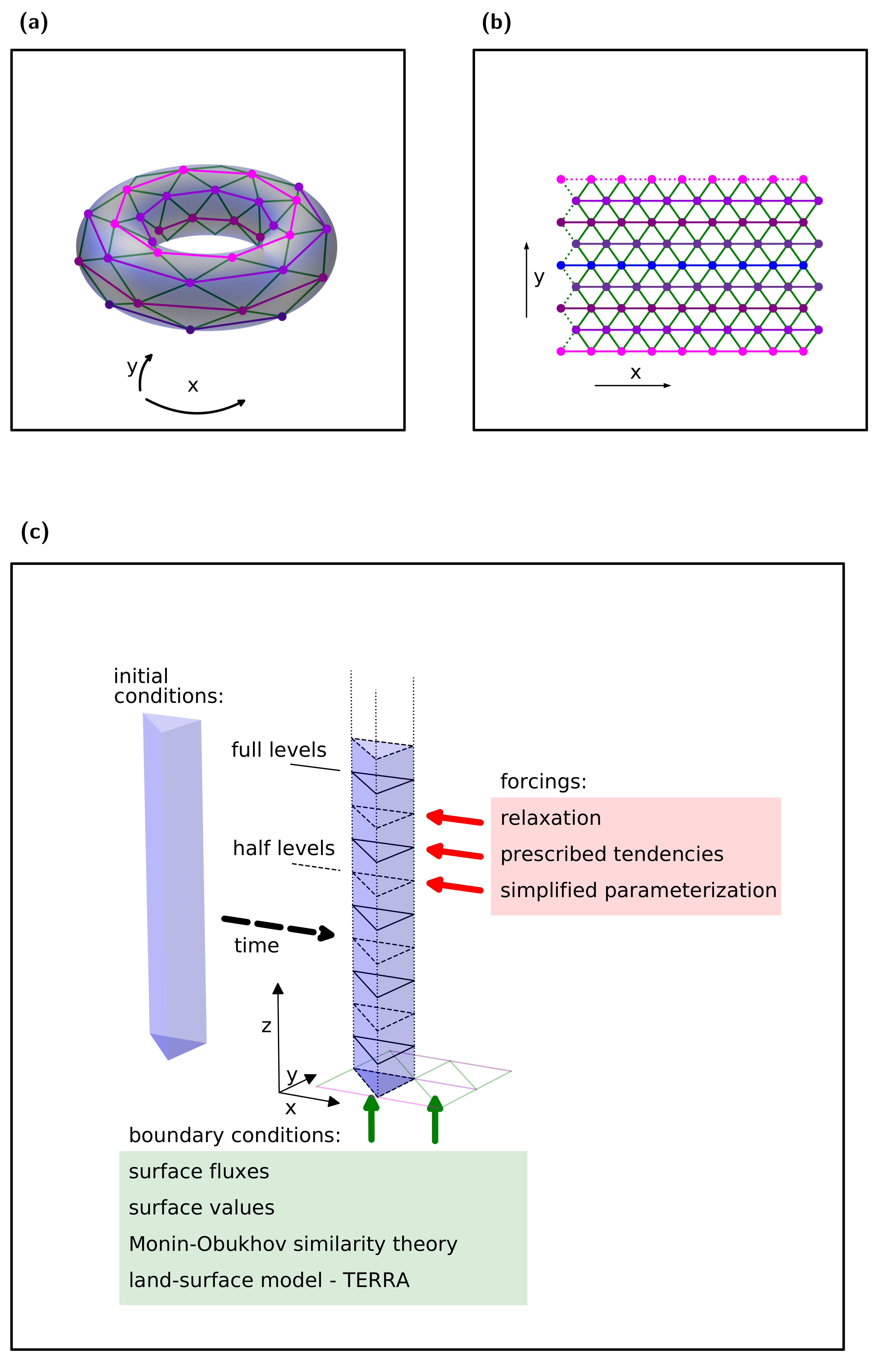
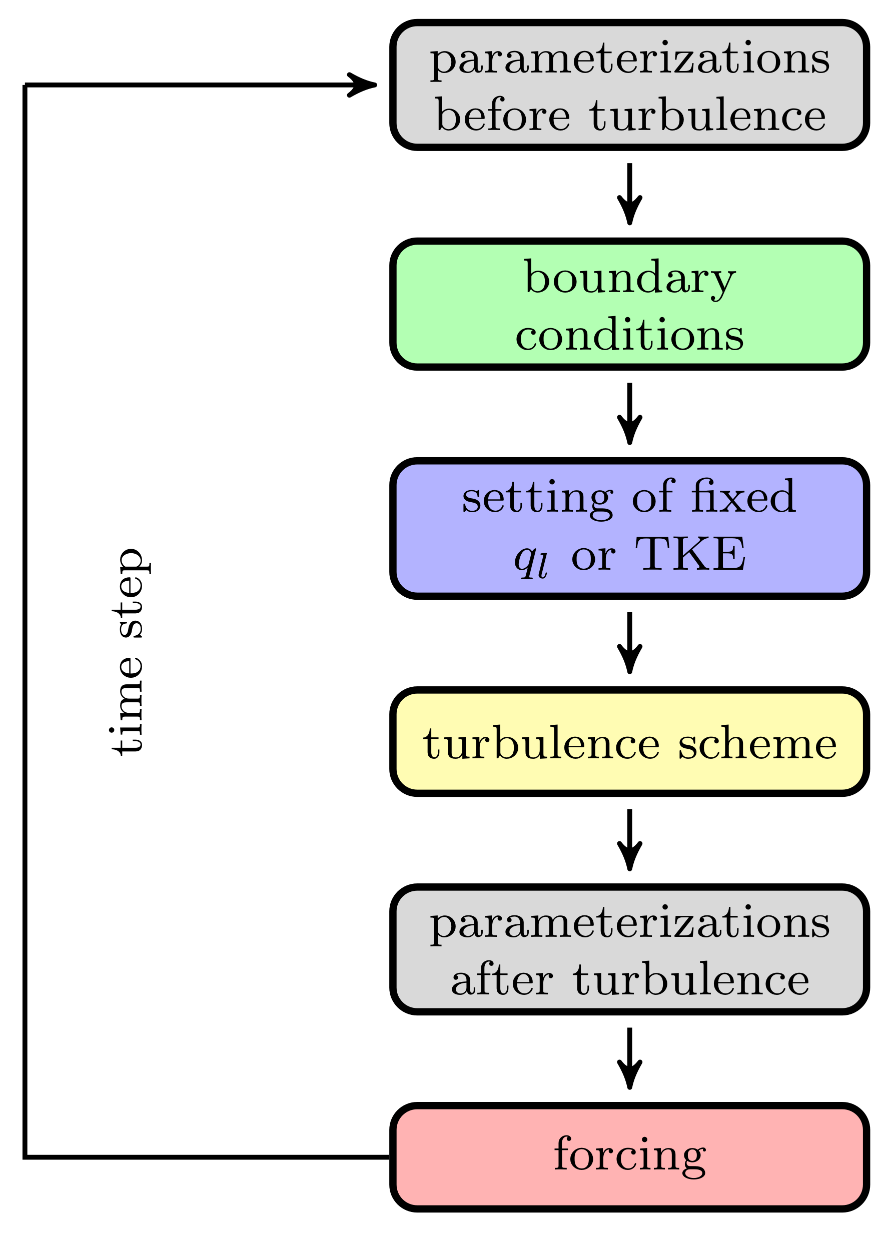
2.1. General Design of ICON SCM

The ICON SCM presented in this study is a particular configuration of ICON, a modeling system for climate studies, global and local numerical weather prediction and large eddy simulation developed by the ICON partner institutions DWD, MPI-M, Karlsruhe Institute of Technology (KIT), and Deutsches Klimarechenzentrum (DKRZ) [25,26,27,29,30]. The ICON model is a fully compressible model that performs computations in grid-point space on geodesic Delaunay grids with C-type staggering. Local refinement of the grid and 2-way nesting are possible. The ICON code has been designed for massively parallel computing architectures. At this point, we refrain from an exhaustive model introduction, but refer to the SCM-specific properties and modifications only. A full description of the ICON model can be found in the referenced articles and at [31].

The ICON SCM includes the full list of NWP physics parameterizations and the same output options as the full ICON model. Generally, the ICON SCM was developed using the same parts of the software code as the three-dimensional ICON model with NWP physics parameterizations (model version operational since 14 April 2021 [32]) and is thus an integral and consistent part of the ICON framework. This allows runing the ICON SCM consistently for the same cases as the full three-dimensional ICON in its different modes: large eddy mode (LEM), cloud resolving mode without deep convection parametrization (CRM), and convection parameterizing mode with deep convection parameterization (CPM). Additionally, the three-dimensional ICON can be run on different geometries: on the globe, on a limited area with open lateral boundary conditions (LAM), and on a limited area with periodic lateral boundaries conditions (PER). A consistent transfer of information across these ICON configurations between the simpler and the more complex ones is possible, which is beneficial for model development.

The ICON SCM is run on a small (at least 4 × 4) pseudo 2D torus grid (see [26] and Figure 1a,b), without interaction between the columns. The dynamics of the model, i.e., the resolved flow, is disabled. This includes also the resolved vertical transport. Instead, the contributions from dynamics are prescribed via external forcing (e.g., subsidence can be prescribed to represent the resolved vertical transport).

All columns are initialized and forced in the same way, hence the evolution of the model is identical in each column. The pseudo 2D torus grid is used instead of a single column, because hereby changes to the original code are minimized and the full infrastructure can be used, which simplifies code maintenance.

Note, however, that the introduction of forcing and prescription of boundary conditions requires additional input for ICON SCM. This information together with the initial conditions of the model are contained in a single NetCDF file, which is read at the start of the simulation. This setup allows preparation of new cases without the need to modify the source code of the model. An internationally coordinated initiative to make the case configurations for SCM and LEM comparable and interchangeable among various models via a standardized NetCDF format is ongoing [33]. ICON is part of this initiative and it is planned to adapt the NetCDF format for ICON SCM accordingly, as soon as the final unified format is defined.

2.2. Forcing and Surface Boundary Conditions

As dynamics is disabled in the SCM, forcing that represent contributions of these parts of the 3D model must be added. These so-called large-scale forcing, together with forcing representing additional non-parameterized sub-grid scale processes, can be introduced by two main methods: relaxing a model variable towards a prescribed value or by prescribing tendencies:

$$\begin{array}{ccc}\hfill \mathrm{relaxation}:{\left(\Delta \psi \right)}^{\mathrm{total}}& =& {\left(\Delta \psi \right)}^{\mathrm{model}}-\left({\psi }^{\mathrm{model}}-{\psi }^{\mathrm{prescribed}}\right)\frac{\Delta t}{\tau }exp\left[-\frac{\Delta t}{\tau }\right],\hfill \end{array}$$

(1)

$$\begin{array}{ccc}\hfill \mathrm{prescribed}\mathrm{tendencies}:{\left(\Delta \psi \right)}^{\mathrm{total}}& =& {\left(\Delta \psi \right)}^{\mathrm{model}}+{\left(\Delta \psi \right)}^{\mathrm{prescribed}},\hfill \end{array}$$

(2)

where $\psi$ represents a prognostic variable, $\Delta t$ is the time step, $\tau$ is the relaxation time scale, $\Delta \psi$ is the change in variable $\psi$ during one time step. Superscript `model’ indicates the tendency given by all active parts of the model, superscript `prescribed’ indicates the prescribed values or tendencies, and superscript `total’ indicates the tendency resulting from both contributions.

Method (1) ensures that the SCM follows the prescribed large-scale evolution of the flow, but that it still has a certain freedom on shorter time scales and particularly at lower levels, i.e., in the atmospheric boundary layer. The strength of the external forcing is controlled by the relaxation time-scale, which can be height dependent. The influence of the active model components on shorter and smaller scales can hence be studied in a well-defined manner. The large-scale evolution is usually driven by a regular NWP model. The advantage of the relaxation method is the rather simple way of obtaining the forcing data, because only time series of the prescribed variables are required, without the need of specifying the contribution from individual processes to their evolution.

Method (2), prescribing tendencies, is more delicate, since the SCM is less restricted. The prescribed tendencies correspond either to the large-scale advection or to processes which are not parameterized in the given setup of the SCM, e.g., radiative forcing. The overall SCM evolution is a result of contributions from prescribed tendencies, surface boundary conditions and the active physical parameterizations that respond to the external forcing. In this way, responses and interactions of the active components can be studied, like feedback mechanisms or conservation properties of the SCM. As it is rather difficult to extract an accurate estimation of tendencies from three-dimensional large-scale models, the prescription of tendencies is usually only used in idealized experiments, although it can also be used in semi-realistic experiments. Depending on the situation, a combination of both methods is possible.

In addition to the two main methods mentioned above, forcing can be prescribed in a more integrated way, where the forcing reflects the current state of the model. Particularly, the influence of large-scale subsidence can be enforced, and the resulting tendencies of the vertically transported quantities are then computed with the help of their current vertical gradients in the SCM. Also, the influence of the large-scale horizontal pressure gradient on the slow evolution can be prescribed via the geostrophic wind. Furthermore, a new simplified parameterization can be introduced into the model instead of an existing parameterization. Currently, this is for example the case for the simplified parameterization of radiation that is used in the DYCOMS-II stratocumulus case [34].

The surface boundary conditions in ICON SCM can be set up in three main ways: first, by prescribed surface turbulent fluxes; second, by prescribed surface values of the prognostic variables, where the surface turbulent fluxes are computed according to the Monin--Obukhov similarity theory using either the operational surface scheme or a simplified method; and third, by using ICON’s land-surface model, TERRA. In this third case, the surface turbulent fluxes are computed interactively. Alternatively to the prescription of turbulent fluxes, the friction velocity, the roughness length or drag coefficients can be prescribed. The turbulent surface fluxes are then computed according to Monin-Obukhov similarity theory from these parameters. Different boundary conditions can be chosen for individual variables, e.g., prescribed friction velocity for momentum, and prescribed surface values for temperature and moisture. All surface boundary conditions can be prescribed in a time-dependent way. An overview of options for the setup of boundary conditions and forcing in the ICON SCM is displayed in Figure 1c.

For idealized cases, forcing and surface boundary conditions are usually based on data obtained from measurement campaigns. The design of the cases involves a certain level of idealization, which requires a careful analysis of the atmospheric conditions. This approach is suitable for studying selected cases, but it is too demanding for automatic processing. To overcome these limitations, forcing and boundary conditions can be generated from larger-scale climate or numerical weather prediction models [35]. We will refer to cases which are run by such forcing and boundary conditions as semi-realistic cases.

With the ICON SCM, both idealized and semi-realistic cases can be simulated. Currently, the setup for the following idealized cases is available: the continental cumulus case based on the Atmospheric Radiation Measurement (ARM) program [15,36], the trade wind cumulus case based on observations from the Barbados Oceanographic and Meteorological Experiment (BOMEX) [37], the precipitating shallow cumulus convection case based on the Rain in Cumulus over the Ocean (RICO) field experiment [38,39], the drizzling stratocumulus case based on the first research flight (RF01) of the second Dynamics and Chemistry of Marine Stratocumulus (DYCOMS-II) field study [34,40], and a test case based on the GEWEX Atmospheric Boundary Layer Study (GABLS1) project [16,41,42]. Furthermore the setup from stage 1 of the GEWEX demistify-fog project [43], an idealized radiation fog case, is included. It is based on data from the Local And Non-local Fog Experiment (LANFEX) [44,45].

For the evaluation of the radiation scheme, 50 clear-sky columns from the Correlated K-Distribution Model Intercomparison Project (CKDMIP) [46] Evaluation 1 dataset are also included as ICON SCM cases. The CKDMIP project provides exact line-by-line radiation calculations for these columns which can be used as a reference for radiation calculations.

The semi-realistic case can be generated from the operational weather forecasts or analyses of the ICON model, provided by DWD. The computation of the forcing is performed via python scripts according to the procedure described in [35], while the technical implementation of the forcing and parts of the surface boundary conditions is based on the ICON LEM [26,29].

The code of the ICON SCM, together with the configuration for the idealized cases and the python scripts for the generation of the forcing can be accessed after registration at the internal DWD gitlab repository (https://gitlab.dkrz.de/, accessed on 13 July 2021) in the “icon-nwp/icon-nwp-scm-new” branch.

2.3. Large Eddy Simulations

The reference LES data for the idealized cases presented here were obtained from simulations with the MicroHH model [28,47]. MicroHH was chosen, because it is a tested and established reference and provides an external verification to the ICON framework. MicroHH was set up and run according to the published description of the cases, with moist thermodynamics activated in all simulations. A parameterization for radiation and microphysics was only used in the DYCOMS-II case, but deactivated in the other cases.

3. Results

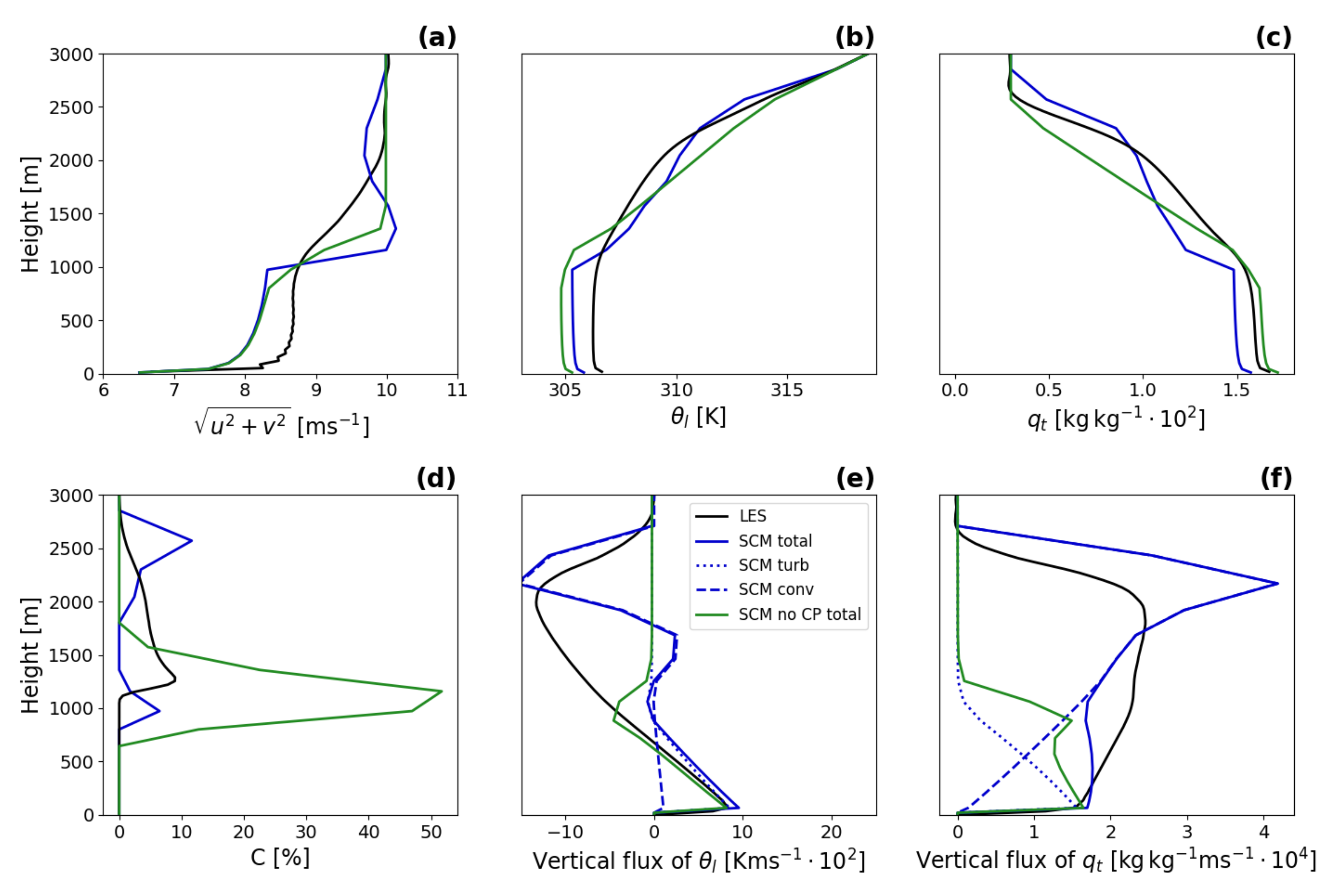
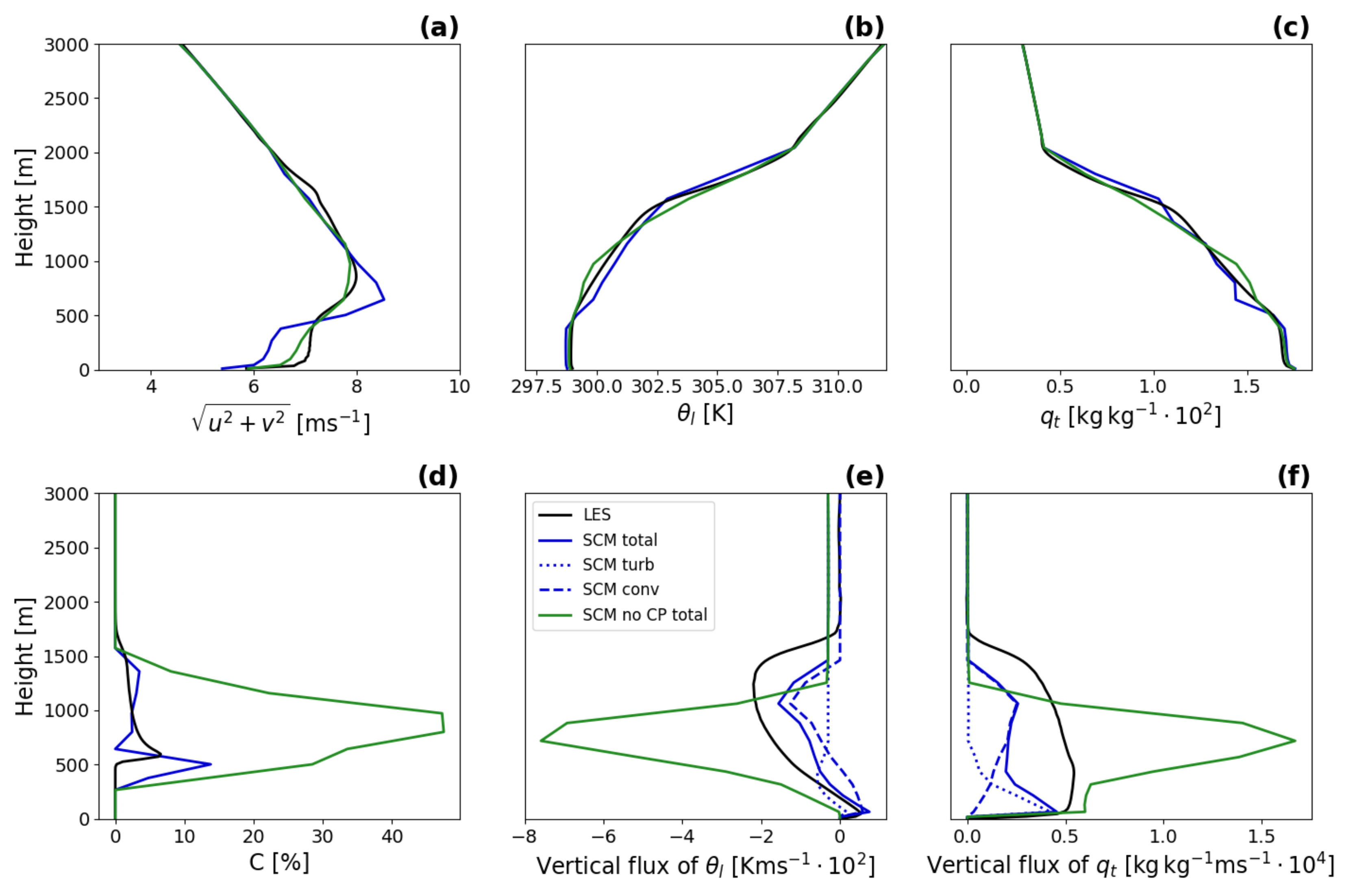
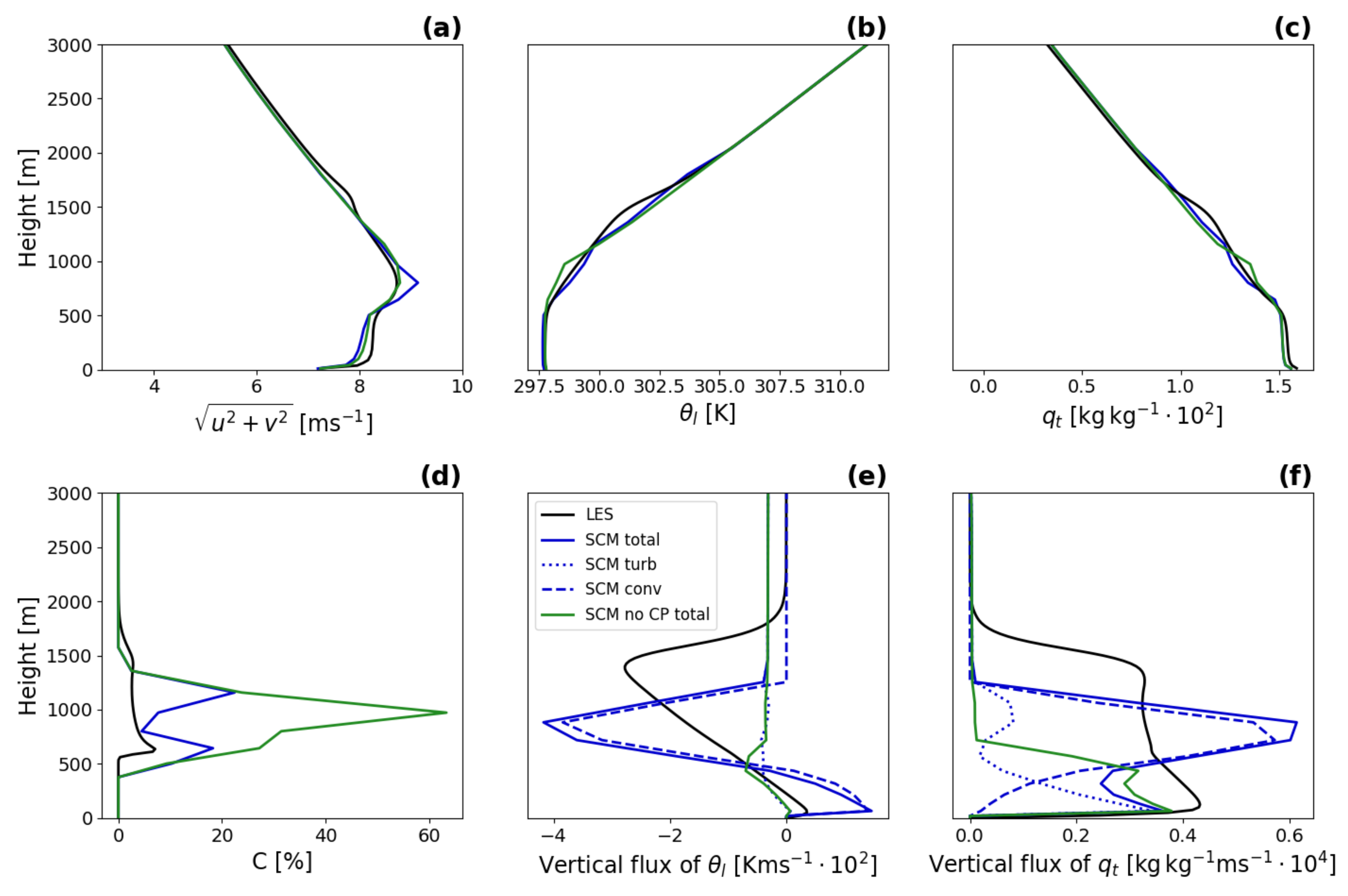
3.1. Study of the Shallow-Convection Parameterization for Three Idealized Cases

As described in Section 1, ICON SCM can be used in several ways. Perhaps the simplest usage of an SCM is the estimation of the tendencies from individual parameterizations. In this subsection, the contributions from the turbulence and from the convection scheme to the evolution of the physical state will be quantified by the analysis of different idealized experiments.

The vertical transport in the convective boundary layer (CBL) is dominated by turbulence and convection. While there is a strong interaction between these two processes and it is not easy to separate them in the CBL, they are traditionally parameterized in two separate schemes in NWP models: the local turbulence scheme and the non-local shallow convection scheme. In the ICON model, the local down-gradient turbulent mixing is parameterized via a turbulent kinetic energy (TKE) closure scheme [48,49] and the convection scheme for both shallow and deep convection is based on a mass-flux scheme, where the entrainment and detrainment include contributions from turbulent and organized parts [50]. To achieve a good overall representation of vertical transport in the CBL, each of these schemes needs to perform its role and they need to interact properly. To analyse this interaction, it is required to extract the individual contributions from each scheme to the model state. This would be difficult in the full ICON model, because of the limitations described in Section 1. Instead, we perform the analysis in the ICON SCM for three idealized shallow convection cases: ARM, BOMEX and RICO, where the behavior of the remaining model components can be prescribed. The instantaneous contributions of the schemes to the tendencies of moisture and temperature can be extracted from the model. However, the resulting model state is given by the cumulative effect of both active schemes and it is not always simple to relate instantaneous changes to the cumulative effect. To infer the cumulative impact resulting only from an individual scheme, experiments need to be performed both with the scheme activated and deactivated. The differences between these two experiments indicate the contribution of that particular scheme. As an illustration, the influence of the shallow convection parameterization is analysed in this way here.

All ICON SCM simulations are performed with a 60 s time step, and a vertical grid as used for the operational numerical weather forecasts, with 90 atmospheric levels, the model top at 75 km and 14 levels in the lowest 2 km. The one-hour mean vertical profiles of wind speed, liquid water potential temperature, ${\theta }_l$, total specific content of water, $q_t$, cloud fraction, C, and the vertical fluxes of ${\theta }_l$ and $q_t$ for the last hour of integration are presented for two model configurations (with and without the convection scheme), along with the vertical fluxes from the turbulence and convection scheme in Figure 2, Figure 3 and Figure 4. The profiles of the SCM simulations are compared to horizontally averaged LES profiles. The LES runs with moist thermodynamics in all cases, while microphysical and precipitation processes are activated only for the RICO case. The setup for the LES are summarized in

Table 1. Horizontal and vertical domain size, horizontal and vertical resolution, and integration time for the LES runs.

Case	Hor. Domain Size	Hor. Resol.	Ver. Domain Size	Ver. Resol.	Integration Time
ARM	12.8 km × 12.8 km	12.5 m	4400 m	31.125 m	10 h
BOMEX	12.8 km × 12.8 km	12.5 m	3000 m	23.44 m	6 h
RICO	8 km × 8 km	25 m	6000 m	25 m	6 h

.

In all three experiments, shallow cumulus clouds develop, apparent in the LES by a cloud fraction with maxima of about 5–10 % (Figure 2d, Figure 3d and Figure 4d). In the SCM, the maximum cloud fraction is higher (up to 60 % for RICO) and the cloud base is lower for all cases and for both SCM configurations, but the overestimation is more pronounced for the configuration with the deactivated convection scheme. The resulting vertical profiles of $q_t$ and ${\theta }_l$ show that both runs have a well-mixed sub-cloud layer, which is in agreement with the LES. This is due to the local down-gradient mixing, which is active in both types of SCM runs as can be seen in the vertical flux profiles.

The convection scheme transports heat and moisture from the sub-cloud layer to the cloud top. Strong gradients of the mean variables near cloud base and cloud top indicate that the convective transport from cloud base to cloud top is too strong. This affects also the cloud fraction, which has too small values in the middle of the cloud layer. However, without the convection scheme, the heat and moisture transported by the turbulence scheme across the cloud base from the sub-cloud layer accumulate above cloud base. Both scalars are further transported upwards by the turbulence scheme, but the rate of transport is too low compared to the LES. This results in the increased cloud fraction and a too small vertical extent of the clouds (same behavior as can be seen in the global NWP ICON [51]). Similar structures can be observed in the vertical profiles of wind speed. If only the turbulence scheme is activated, it computes the fluxes of ${\theta }_l$ and $q_t$ following a down-gradient formulation: they are strong in the presence of gradients and under unstable stratification. As the vertical profiles do not change rapidly, this relationship is visible not only for individual time steps, but also for one-hourly means.

If the convection scheme is activated, the turbulence scheme is less active because the non-local non-gradient mixing of convection reduces most vertical gradients. The overall one-hour fluxes of ${\theta }_l$ and $q_t$ seem to be too weak for the BOMEX case and they do not extend high enough for both the BOMEX and RICO case. This results in the on/off behavior of the convection scheme, which was active in the previous hours of the simulation and would be probably triggered again if the experiment continued. This is also evident from the jagged profiles of the displayed variables.

It can be concluded that the shallow convection parameterization acts as expected by non-locally transporting scalars from the sub-cloud layer to higher levels. However, the convective transport seems to be too strong and too sparsely triggered. This behavior could be adjusted by further work, which would include analyses of mass flux, updraft fraction, updraft velocity, entrainment and detrainment in the convection scheme (see e.g., [52,53]). We will not elaborate on this topic any further since it is beyond a simple demonstration of the ICON SCM usage.

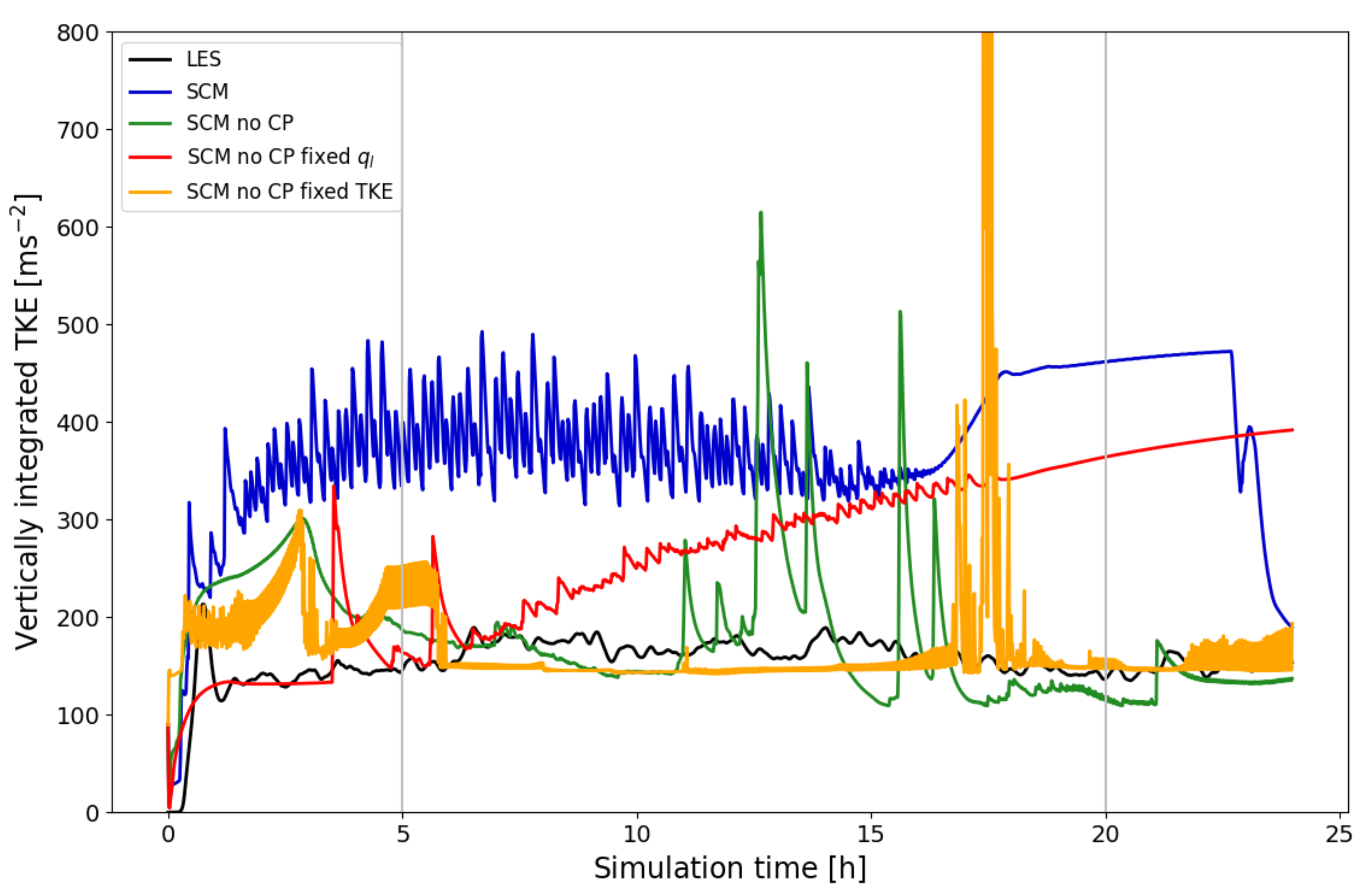
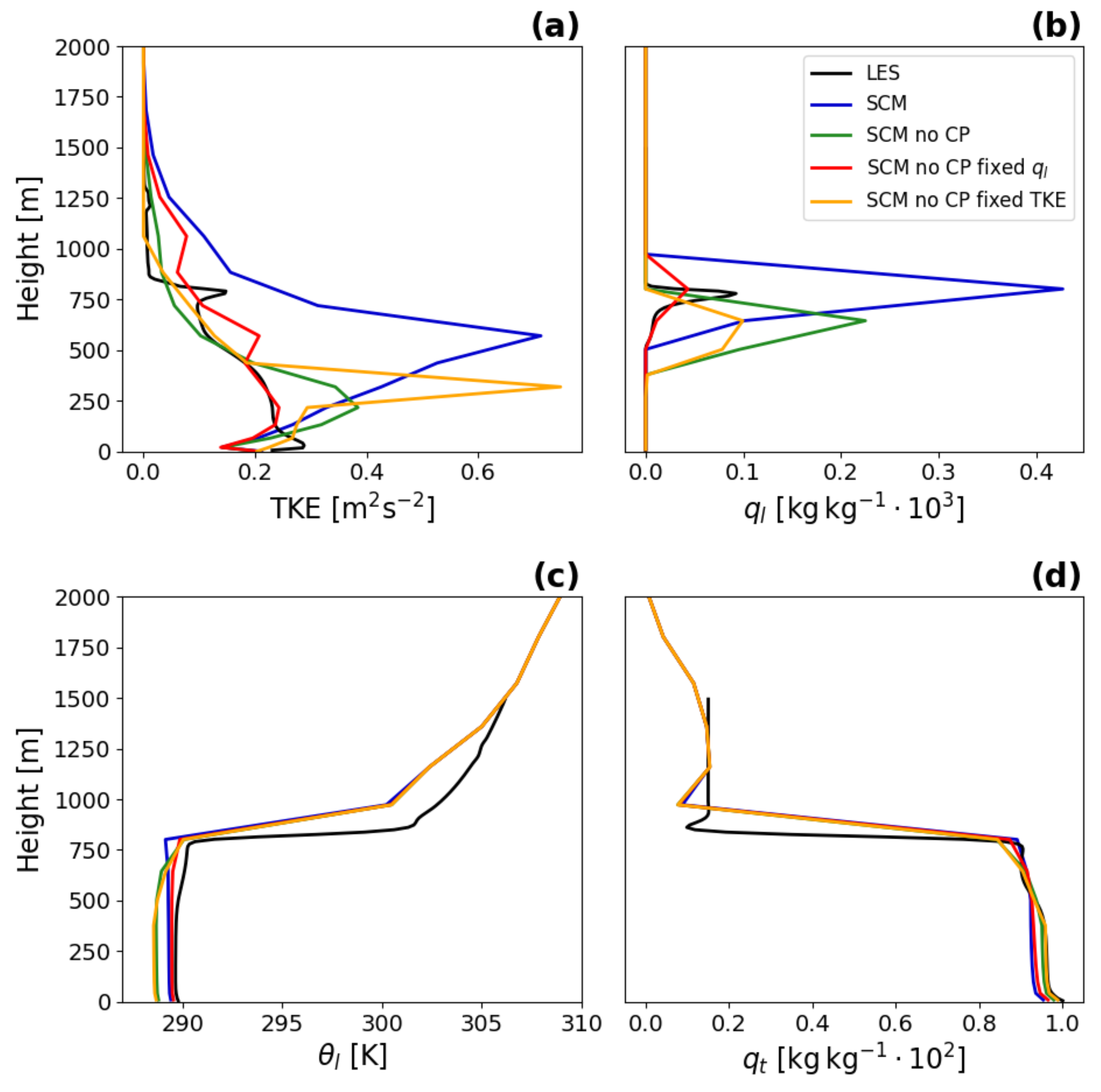
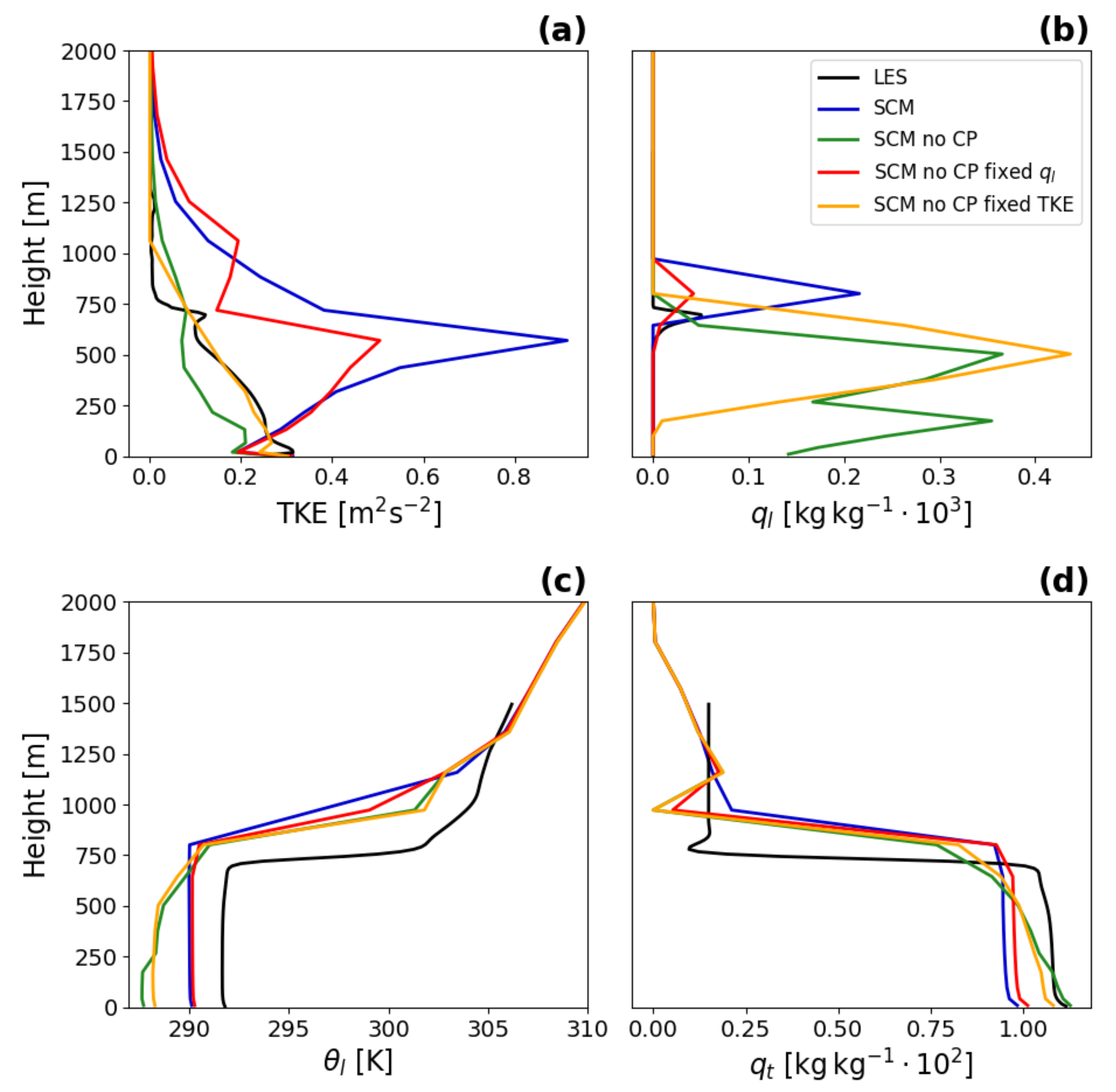
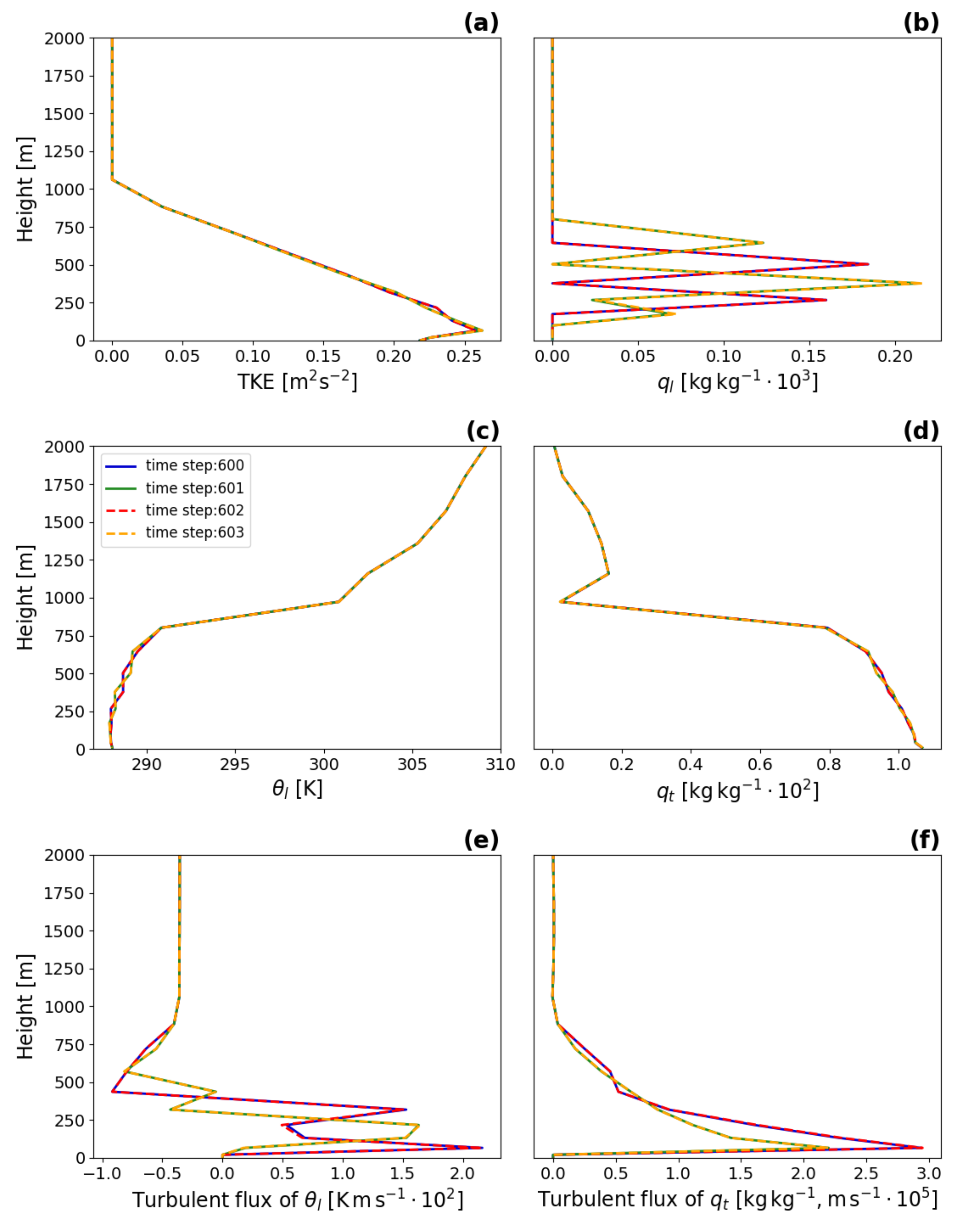
3.2. Feedback Study between Cloud Water Content and Turbulence in a Stratocumulus Case

In this subsection, a more complex usage of the ICON SCM, a study of a feedback mechanism, is demonstrated. For this purpose, we analyze the interaction between cloud water and the intensity of turbulent mixing in the idealized stratocumulus case DYCOMS-II [34,40].

In stratocumulus cases, there is typically an approximate energy balance between entrainment warming, radiative cooling, and heating from the surface fluxes [34]. At the same time there is a moisture balance between entrainment drying and moistening from the surface. In the DYCOMS-II case, the surface fluxes are fixed and the radiative cooling does not change as long as the cloud remains optically thick. Thus, the balance is given by the entrainment rate and the cloud liquid water amount. This balance can be observed in the LES run in Figure 5 and Figure 6 (black line), in which the evolution of vertically integrated TKE (ITKE), a measure of the intensity of turbulence mixing, and the liquid water path (LWP) are depicted.

In the ICON model, there is no explicit entrainment parameterization for stratocumulus cases. Instead, the TKE scheme models the turbulent transport of heat and moisture across the cloud top. The TKE is modified by phase changes of water via the buoyancy production term, which increases when water vapour condensates and clouds are formed [54,55]. With the increase of TKE, the turbulence mixing in and near clouds intensifies, leading to entrainment across the cloud top, decreasing cloud moisture and causing evaporative cooling. The change in the thermodynamic state of the CBL slows down or stops the condensation, resulting in a decrease of TKE in the cloud region. With the subsequent decrease in turbulent mixing, moisture and its gradients increase again due to the constant surface flux. This leads again to condensation and the cycle repeats.

It is obvious that this mechanism can lead to a drift of the model from an equilibrium state, or to oscillations around the equilibrium state, if the modeled links between turbulent mixing and cloud liquid water content are unbalanced or not sufficiently accurate. It is desirable to avoid the model drift and spurious oscillations, because both conditions decrease the accuracy of the simulations and the oscillations can generate additional energy in the system. Hence, the modeling of this mechanism should be studied in detail. To observe such behavior in a three-dimensional model is difficult, because the physics interact with the dynamics and the volume of diagnostic data is very large if it is written to disk at each time step. Therefore, an SCM is the ideal tool to study such interactions.

For all DYCOMS-II experiments, ICON SCM runs as in the previous study (Section 3.1) with 90 vertical levels, having 14 levels in the lowest 2 km, and a time step of 60 s. A simplified radiation scheme is used, according to the specification of the case (see [34,40]). The LES runs with moist thermodynamics, microphysical and precipitation processes, and the simplified radiation scheme. The domain size is 4.096 km × 4.096 km in the horizontal and 1.5 km in the vertical with horizontal and vertical grid spacings of 32 m and 11.72 m, respectively.

To capture the overall behavior of the ICON SCM in the DYCOMS-II case, the evolution of ITKE and LWP are displayed in Figure 5 and Figure 6, respectively. More details about the vertical structure of the CBL can be seen in the one-hourly mean vertical profiles of total specific water content, liquid water potential temperature, TKE and liquid water content ($q_l$) after 5 and 20 h of integration in Figure 7 and Figure 8, respectively.

The ICON SCM (blue line) is in good agreement with the LES in terms of the vertical profiles of $q_l$ and ${\theta }_l$ for the first 5 to 10 h of the simulation (see Figure 7). Liquid water content is higher than for the LES, but it is within the range of results of other SCM simulations [34]. The inversion across the top of the CBL is not as sharp as in the LES, which can mostly be explained by the coarser vertical resolution of the SCM. However, the ICON SCM slowly drifts in terms of the LWP, first increasing slightly and then decreasing until the CBL is cloud-free after about 23 h of simulation (Figure 6). TKE is significantly overestimated, which can be seen in both the vertical profiles and the evolution of ITKE (Figure 5). The mean value of ITKE does not change significantly until cloud-free conditions are met, which suggest that the main source of TKE and the reason for its overestimation is due to the presence of clouds.

Until about 15 h of simulation, an oscillation in the evolution of ITKE and LWP can be observed for the ICON SCM. This can be related to the oscillation mechanism described above. However, the growth of the CBL, and the vertical transport in the upper part of the CBL is not caused only by the turbulence scheme, but also by the shallow convection parameterization. This can be demonstrated when the shallow convection parameterization is turned off. The vertical transport in the upper part of the CBL in the experiment without shallow convection parameterization is weaker and the CBL not completely mixed, which causes a cooling of the CBL, and an accumulation of liquid water in the whole CBL (see Figure 7 and Figure 8). At the same time, the ITKE oscillation almost disappears and the oscillation of LWP increases its frequency and amplitude.

The shallow convection parameterization was not designed to be active in stratocumulus conditions (see [34]), thus it probably compensates for the insufficient mixing by the turbulence scheme. This complicates the investigation of the feedback, but also demonstrates that detailed understanding of the model is important to isolate the influences of individual parameterizations. In this spirit, we will limit our remaining analyses of the feedback to the model setup with the deactivated shallow convection parameterization.

In order to narrow down the cause of the drift of the system and the oscillations, we will investigate the two links of the feedback mechanism separately, i.e., (1) the influence of turbulent mixing on cloud liquid water content, and (2) the influence of cloud liquid water content on turbulent mixing. In the SCM this can be achieved by fixing one of the components of the feedback. In our case, (1) the vertical profile of TKE (orange curve in Figure 5, Figure 6, Figure 7 and Figure 8) or (2) the vertical profile of $q_l$ (red curve) is fixed during the whole integration of the model.

The prescribed profiles approximate the equilibrium profiles obtained from the LES after 10 h of integration. If the active link of the feedback is modeled properly, the SCM should evolve towards an approximate equilibrium state as well. Technically, the profiles of TKE and $q_l$ are set to the fixed profiles every time step before the subroutine for the computation of the turbulent fluxes is called (see Figure 9). This kind of fixation of the profiles still leaves some freedom to the model, because the turbulent tendencies in the given time step can influence the profiles. This can be seen in the temporal deviation of the LWP and the ITKE from their fixed values and also in the vertical profile of TKE in Figure 7.

Comparing the two fixed cases, an approximate equilibrium for the LWP and ITKE is achieved only for the case (2) with fixed $q_l$. The vertical profiles for fixed $q_l$ are close to the vertical profiles of the SCM run with the shallow convection parameterization (blue curve), with the exception of the TKE profile. The TKE profile after 5 and 20 h shows that the TKE is closer to the LES profile in the CBL. There is still an overestimation caused by the generation of TKE through buoyancy in the presence of clouds. Because $q_l$ has values comparable to the LES, the resulting TKE is improved. Still, considerably more TKE is required than in the LES to receive sufficient cloud top entrainment to get close to the stratocumulus equilibrium state (Figure 5, red curve). In other words, the two links of the feedback are not balanced. Without fixing $q_l$ the balance is not established. If the shallow convection parameterization is turned on, sufficient transport across the CBL top is ensured, but the scheme slowly pushes the model to a cloud-free state. Of course, without the interference of clouds in the cloud-free state an equilibrium can be achieved.

The imbalance between the links is confirmed in experiment (1) with fixed TKE (orange curve), where no equilibrium is reached, because the prescribed TKE is too low to cause sufficient mixing across the cloud top. Therefore, the result with fixed TKE resembles the experiment where no shallow convection parameterization was used (green curve).

Before an equilibrium is reached, the oscillations in the ITKE and LWP are most likely caused by prescribing a fixed profile of $q_l$ and TKE - the model tries to evolve, but the fixation forces it back. In an equilibrium state, the oscillations should vanish if one part of the feedback is deactivated. Indeed, that is the case in the fixed $q_l$ case (2). This means, that oscillations could be removed if the links between TKE and $q_l$ were more accurate.

In contrast, there is a continuous presence of the LWP oscillations in the fixed TKE case (1) even for time periods when the ITKE is almost constant. This indicates that there is another source of oscillations. For more details, we look at the individual vertical profiles of TKE, $q_l$, ${\theta }_l$, $q_t$, and the turbulent flux of $q_t$ and ${\theta }_l$ (see Figure 10) at several time steps after about 10 h of integration. The profiles demonstrate that the oscillations are related to the turbulent fluxes, but are not caused by the changes in TKE (since TKE is fixed). The character of the oscillation, (period of two time steps, bounded amplitude of oscillations) exhibit similar features as the so called “fibrillations” [56] that arise from the feedback between the gradient Richardson number and the vertical profiles of the diffused variables, $q_t$ and ${\theta }_l$.

From this brief demonstration, it can be concluded that the ICON model performs sufficiently well in the first 10 h of the integration when the shallow convection parameterization is turned on. However, a more detailed investigation with the help of the SCM shows that the individual schemes and their components do not perform as expected. Specifically, the shallow convection parameterization, which was not designed to be active in stratocumulus cases, compensates for the weak turbulent mixing in the upper part of the CBL. It also prevents oscillations generated by the turbulence scheme. The SCM study identifies two possible sources of these oscillations: a feedback between TKE and the clouds, and the interaction between the gradient Richardson number and the vertical profiles of the diffused variables.

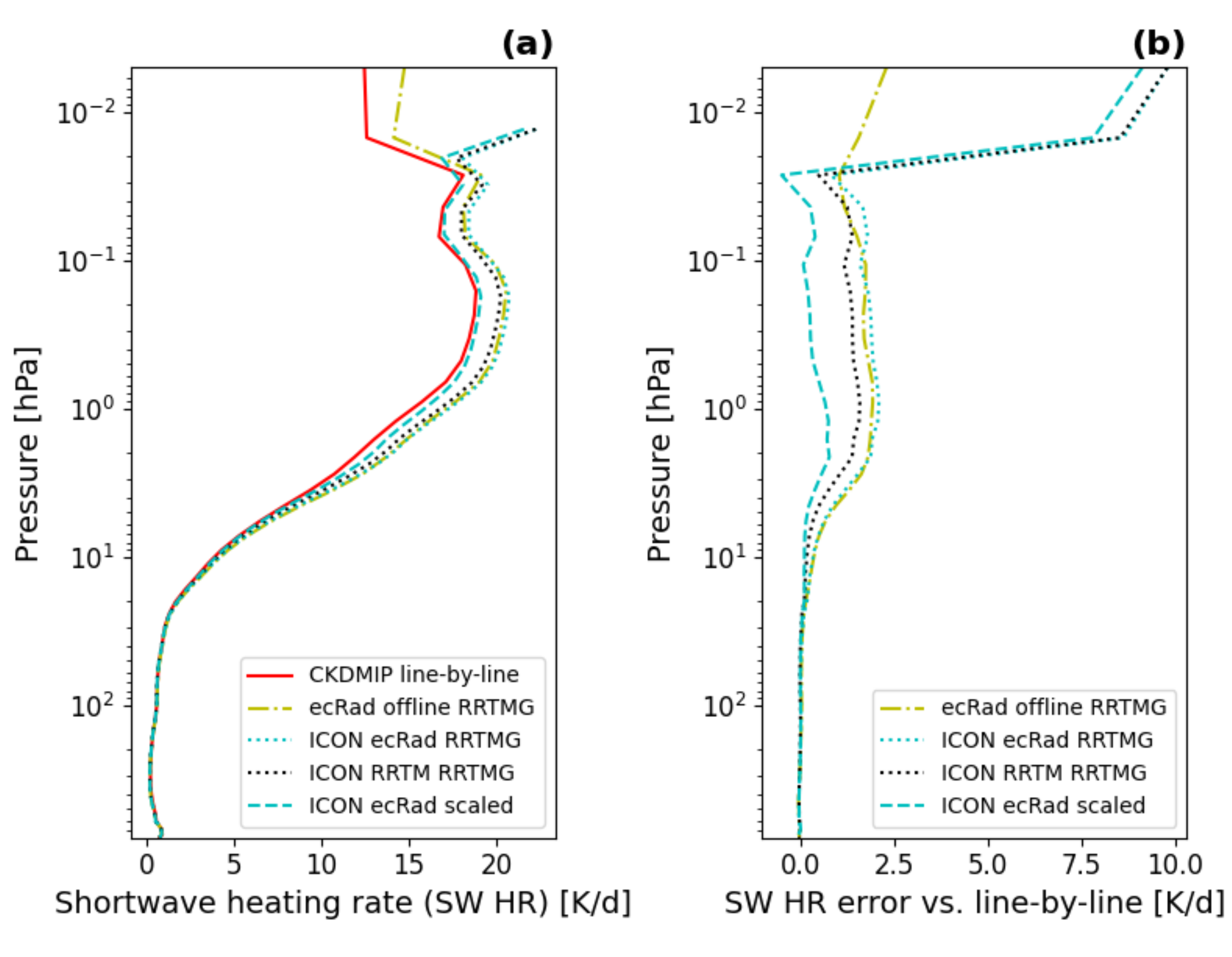
3.3. Evaluation of Clear-Sky Radiation and Improvement of the Solar Spectrum

Another illustrative example of SCM usage is the evaluation of radiation schemes, which are the key drivers of the energy balance in models. Clear-sky gas absorption and emission are challenging to model in a numerically efficient way, since they vary very strongly with wavelength. Line-by-line radiation calculations using millions of spectral lines are highly accurate compared to observations [57], but are only possible for selected test columns.

In this subsection, we compare the ICON SCM using both the newly implemented ecRad radiation scheme [58,59] and the older RRTM radiation scheme to line-by-line calculations performed by Hogan and Matricardi [46] in CKDMIP [60] using the Line-By-Line Radiative Transfer Model (LBLRTM) [61], and to CKDMIP offline ecRad calculations, for 50 clear-sky test columns representative of the global atmosphere (the CKDMIP Evaluation 1 dataset). Such a comparison provides a benchmark for the radiation schemes, indicates their weaknesses, and can lead to improvements. We will focus specifically on the influence of the solar spectrum on clear-sky radiative heating.

Both ecRad and the RRTM radiation scheme use the global model version of the Rapid Radiative Transfer Model gas optics scheme (RRTMG) [62,63], which determines the radiation model spectral intervals, and the spectral distribution of solar radiation. The RRTMG version used in ecRad is equivalent to RRTMG_SW v. 3.9 in the shortwave and RRTMG_LW v. 4.85 in the longwave. We have adapted the CKDMIP profile data to the ICON SCM input format and interpolated them onto the ICON model levels. We consider radiation results for the first time step, in atmospheric conditions identical to the input profile used in the line-by-line calculations.

Comparison of shortwave heating rates for one test profile in Figure 11 shows that when using the original RRTMG gas scheme, both offline ecRad and ICON SCM, with both ecRad and the old RRTM radiation scheme, overestimate shortwave heating in the stratosphere, between 10 and 0.03 hPa. The reason is that the spectral distribution of incoming solar in the RRTMG gas optics, based on the data of Kurucz [64], is outdated [65,66]. More precise and up-to-date observations of the solar spectrum by Coddington et al. [67] reveal more visible and less ultraviolet sunlight. Since stratospheric heating is mostly due to absorption of ultraviolet light by ozone, using the outdated spectrum results in too much stratospheric shortwave heating, even when the total amount of incoming solar radiation is unchanged. The evaluation of offline ecRad in CKDMIP also showed this bias [60]. We have implemented the scaled corrected solar spectrum of Hogan et al. [66], in agreement with Coddington et al. [67], for ecRad in ICON (as this is the new radiation scheme in ICON, replacing the old RRTM scheme). Using this scaled spectrum, ICON SCM with ecRad agrees much better with the line-by-line results. Results for other test profiles in the dataset are qualitatively very similar.

Comparing ICON SCM calculations to a line-by-line radiation model on test profiles has allowed us to confirm and correct a bias in stratospheric heating, improving stratospheric temperature in ICON, which feeds back on atmospheric circulation. Using ecRad and the scaled solar spectrum, ICON SCM results agree closely with the line-by-line calculations, demonstrating that clear-sky interaction between radiation and gases and the resulting heating rates are well represented in the new ICON setup.

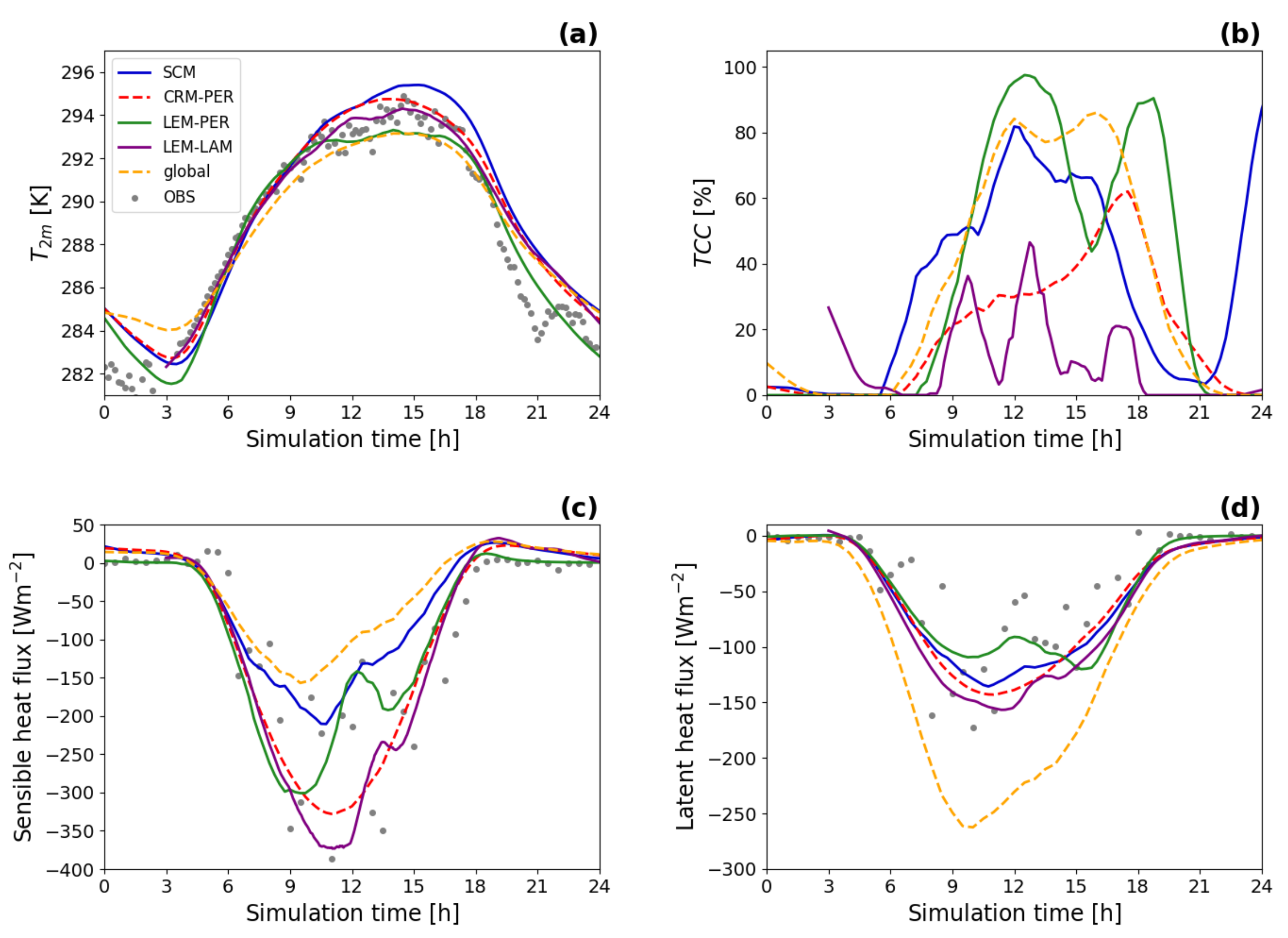
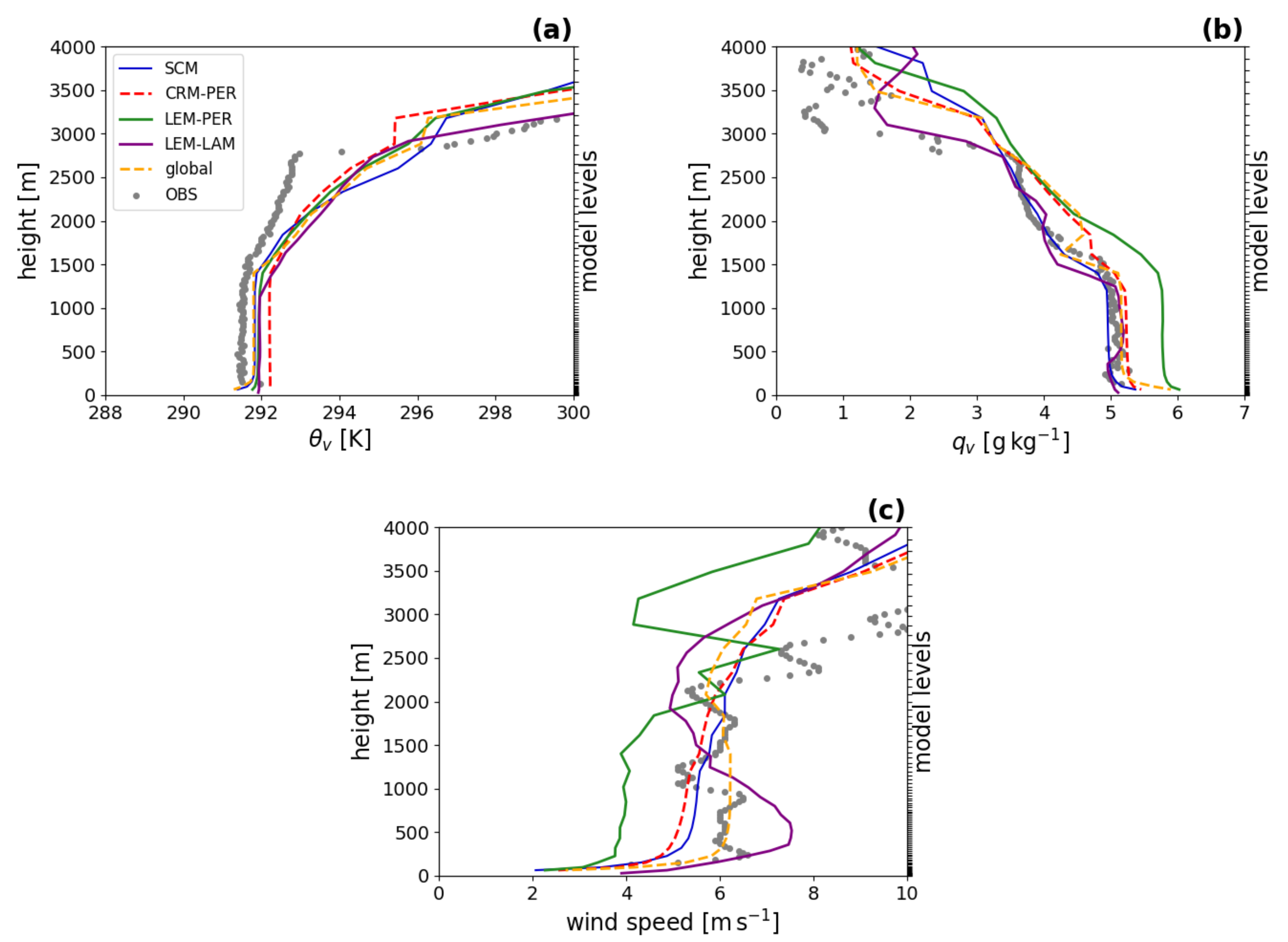
3.4. Semi-Realistic Simulations

SCMs have a long tradition in aiding model development by recreating specific or typical model conditions from a 3-D model in a simpler 1-D environment. Such a setup of the SCM can help in parameterization development, but can also help with debugging model errors, such as an escalating oscillation.

In order to facilitate this approach, the ICON SCM has a native mode, where it is driven by the data originating from the full 3D ICON model on a single point. This mode can also be used when running the land-surface model, in which case the soil moisture and soil temperature profiles can be also prescribed according to the full ICON model.

An advantage of the native mode is the ability to run the SCM, the CRM-PER and the LEM-PER on a torus grid with identical forcing, which in turn closely mirrors the column output from the global ICON run that created the forcing. This capability is demonstrated here on a summer land convection case from the observational Field Experiment on Submesoscale Spatio-Temporal VAriability in Lindenberg (FESSTVaL (http://fesstval.de/, accessed on 13 July 2021)) in eastern Germany on 12 July 2020 starting at 00 UTC.

To create the forcing data, a global ICON simulation at 40 km horizontal resolution was performed, based on the model version operational since 14 April 2021 [32], including the ecRad radiation scheme from ECMWF. An SCM simulation was then set up to mirror the settings in the global run with the identical code and namelist, including the interactive land-surface model TERRA.

To keep the SCM simulation close to the large-scale conditions in the global ICON, nudging was used for temperature, water vapor and the horizontal wind components with a relaxation time-scale of two hours towards the forcing data. Experience with the SCM shows that a two-hour relaxation time-scale is not too restrictive and allows the model to evolve on smaller time scales in a different way than in the driving model.

For the SCM setup, the dynamics was turned off. The LEM-PER and CRM-PER simulations on a torus grid were run with the same forcing setup as the SCM, but with the model dynamics active. A torus grid of 50 × 50 points with 200 m horizontal resolution was used for the LEM-PER, and a torus grid of 100 ×100 points with 2 km horizontal resolution was used for the CRM-PER. For the LEM-PER and the CRM-PER simulations, horizontally averaged (over the domain) data are used in the comparison in Figure 12 and Figure 13. The vertical grid is identical in all three configurations.

Additionally, the LEM was run on a more realistic LAM geometry (LEM-LAM). Initial and lateral boundary conditions were taken from the operational weather forecast of the German Weather Service at 6.5 km horizontal resolution. The simulation was run in a 1-way nested configuration, refining the horizontal grid from 628 m to 314 m and 157 m in the innermost domain. The size of the circular domains was reduced with every refinement step from about 200 km diameter for the coarser domain and about 25 km for the innermost domain. High frequency output for the SCM location (one grid-point), was saved for the comparison in Figure 12 and Figure 13.

The time-series of 2 m temperature, cloud cover, and surface fluxes for the 12 July 2020 are compared between the consistently forced SCM/LEM-PER/CRM-PER on a torus grid, the global ICON, the LEM on a LAM grid, and tower observations at the Falkenberg site in Figure 12. A strong diurnal cycle with moist convection is visible for all simulations.

The results for individual simulations are similar and generally in good agreement with the observations, but differences are clearly visible. The biggest differences between the simulations are in cloud cover, because of its complexity (non-linearities in moist processes and predictability reasons). The less continuous evolution of cloud cover for the LEM-LAM simulation is probably caused by horizontal variability of the cloud cover since only one grid-point from the LEM-LAM domain was chosen for this comparison. We will not analyse and interpret the results in detail here.

The vertical profiles in Figure 13 show similar results. The simulations are compared with radio sounding observations at the meteorological observatory Lindenberg. All simulations have realistic vertical profiles with individual fluctuations. Clearly, all simulations overestimate ${\theta }_v$ in the cloud layer, which could indicate an underestimation of the vertical transport in this layer. The height of the boundary layer agrees well with the observations.

An interesting result is that the activation of the dynamics in the CRM-PER on a torus grid significantly helps the vertical transport, which is underestimated in the SCM (SCM and CRM-PER differ only in the activation of dynamics).

A consistent comparison of model configurations like the one presented here, can be helpful in model development across the whole hierarchy of ICON configurations. The LEM-PER and LEM-LAM can be used as additional references in addition to the observations. The former is more idealized, because it is forced by the simplified SCM setup, but as a result it can be consistently compared to the SCM and the CRM-PER. The LEM-LAM contains information about the horizontal variability (boundary conditions and lateral conditions), hence it is more realistic. The SCM can be used to isolate the possible problems in a single column. The CRM-PER on a torus, the simulations on the LAM grid, and the simulations on the global grid can be used to asses the contribution of 3D processes in the NWP setups, especially those due to dynamics.

4. Conclusions

We have presented the single-column mode of the ICON model, the ICON SCM. The primary purpose of the ICON SCM is to use it as a tool for research, model development and evaluation. The ICON SCM is suitable for model development, as it offers a well-controlled environment, where the influence of large-scale forcing, dynamics and selected physical parameterizations can be prescribed. Additionally, the ICON SCM has a small computational cost and a low storage demand.

The ICON SCM can be run for already prepared well-established idealized cases or for semi-realistic cases based on analyses or model forecasts. New cases can be easily prepared by the modification of the input NetCDF file. We have demonstrated the usage of the ICON SCM for different idealized cases of shallow convection, stratocumulus clouds, and radiation. The ICON SCM was also tested in a semi-realistic setup together with other configurations of the ICON model.

First, ICON SCM simulations have been presented for three idealized cases of shallow convection: ARM, BOMEX, and RICO, each with an activated and deactivated convection scheme. The aim was to estimate the contribution of the convection scheme to the vertical transport in the CBL. It was shown that the shallow convection parameterization acts as is expected by non-locally transporting scalars from the sub-cloud layer and the cloud base to higher levels. However, the convective transport seems to be too strong and triggered too infrequently.

Then, we showed simulations for the idealized stratocumulus case DYCOMS-II. The focus was on the feedback mechanism between cloud water and the intensity of turbulent mixing, while the convection scheme is deactivated. The individual links in the feedback mechanism, the influence of turbulent mixing on cloud liquid water content, and vice versa, were analysed by running ICON SCM with either a fixed TKE profile or a fixed $q_l$ profile. The results indicate that the two links of the feedback are not balanced, leading to a slow drift of the model and to oscillations. The situation is mitigated when the convection parameterization is activated, which increases the transport in the upper part of the convective boundary layer and removes oscillations. Additionally to these results, a secondary source of oscillations was identified, which is probably caused by the interaction between the computation of the gradient Richardson number and the vertical profiles of diffused variables.

Next, the ICON SCM was used for the evaluation of the radiation schemes RRTM and ecRad, on a clear-sky test columns. Comparison with the reference line-by-line radiation calculations showed a bias in a stratospheric heating rates due to an outdated solar spectrum in the RRTMG gas scheme. The clear-sky results of ecRad in ICON SCM were improved when the scaled solar spectrum of Hogan et al. [66] was used.

Finally, the ICON SCM was run in a semi-realistic setup with the land-surface model (TERRA), driven by the forecast of the ICON global mode for one selected grid point. The LEM-PER mode and CRM-PER mode on a torus grid were also tested on the same atmospheric conditions. Both used the same forcing as the SCM. Additionally, ICON LEM was run in a LAM configuration (LEM-LAM) as a reference for the simulations. Comparison across this hierarchy of ICON configurations showed similarities, but also individual differences, mainly arising from shorter temporal and spatial scales. Such consistent comparisons of model configurations can be helpful in model development, where each of the modes can be used for a specific task: the LEM modes (LEM-PER and LEM-LAM) can be used as a reference, the SCM can be used to isolate the possible problems in a single column; and the CRM-PER mode on a torus grid, and simulations on the LAM grid, and on the global grid can be used to asses the contribution of 3D processes.

The ICON SCM and the associated CRM-PER mode and LEM-PER mode on a torus grid will be implemented into the operational version of the ICON code. Specific technical aspects of the ICON SCM were not discussed in this paper. More details will be published in a technical documentation. There are several idealized cases that can be run with ICON SCM. In order to expand the number of cases, we plan to switch the NetCDF format of the input file to an unified standardized format [33], which will enable the usage of readily prepared cases from the scientific community.

Currently, the ICON SCM is not able to run with the tile approach, which enables to account for the subgrid-scale heterogeneity of land-surface types. We plan to introduce this important option in the future development of the code.

References

1. Stull, R. An Introduction to Boundary Layer Meteorology; Springer Netherlands: Dordrecht, The Netherlands, 1988. [Google Scholar]
2. Stensrud, D.J. Parameterization Schemes: Keys to Understanding Numerical Weather Prediction Models; Cambridge University Press: Cambridge, UK, 2007. [Google Scholar] [CrossRef]
3. Wyngaard, J.C. Toward Numerical Modeling in the “Terra Incognita”. J. Atmos. Sci. 2004, 61, 1816–1826. [Google Scholar] [CrossRef]
4. Chow, F.; Schär, C.; Ban, N.; Lundquist, K.; Schlemmer, L.; Shi, X. Crossing Multiple Gray Zones in the Transition from Mesoscale to Microscale Simulation over Complex Terrain. Atmosphere 2019, 10, 274. [Google Scholar] [CrossRef] [Green Version]
5. Randall, D. Use of single-column models and large-eddy simulations together with field data to evaluate parametrizations of atmospheric processes. In Proceedings of the Diagnosis of Models and Data Assimilation Systems, ECMWF, ECMWF, Shinfield Park, Reading, UK, 6–10 September 1999; pp. 285–318. [Google Scholar]
6. Hourdin, F.; Jam, A.; Rio, C.; Couvreux, F.; Sandu, I.; Lefebvre, M.P.; Brient, F.; Idelkadi, A. Unified Parameterization of Convective Boundary Layer Transport and Clouds With the Thermal Plume Model. J. Adv. Model. Earth Syst. 2019, 11, 2910–2933. [Google Scholar] [CrossRef] [Green Version]
7. Betts, A.K.; Miller, M.J. A new convective adjustment scheme. Part II: Single column tests using GATE wave, BOMEX, ATEX and arctic air-mass data sets. Q. J. R. Meteorol. Soc. 1986, 112, 693–709. [Google Scholar] [CrossRef]
8. Gettelman, A.; Truesdale, J.E.; Bacmeister, J.T.; Caldwell, P.M.; Neale, R.B.; Bogenschutz, P.A.; Simpson, I.R. The Single Column Atmosphere Model Version 6 (SCAM6): Not a Scam but a Tool for Model Evaluation and Development. J. Adv. Model. Earth Syst. 2019, 11, 1381–1401. [Google Scholar] [CrossRef] [Green Version]
9. Baas, P.; Bosveld, F.; Lenderink, G.; van Meijgaard, E.; Holtslag, A.A.M. How to design single-column model experiments for comparison with observed nocturnal low-level jets. Q. J. R. Meteorol. Soc. 2010, 136, 671–684. [Google Scholar] [CrossRef]
10. Lane, D.E.; Somerville, R.C.J.; Iacobellis, S.F. Sensitivity of Cloud and Radiation Parameterizations to Changes in Vertical Resolution. J. Clim. 2000, 13, 915–922. [Google Scholar] [CrossRef]
11. Sušelj, K.; Teixeira, J.; Matheou, G. Eddy Diffusivity/Mass Flux and Shallow Cumulus Boundary Layer: An Updraft PDF Multiple Mass Flux Scheme. J. Atmos. Sci. 2012, 69, 1513–1533. [Google Scholar] [CrossRef]
12. Huang, H.Y.; Hall, A.; Teixeira, J. Evaluation of the WRF PBL Parameterizations for Marine Boundary Layer Clouds: Cumulus and Stratocumulus. Mon. Weather Rev. 2013, 141, 2265–2271. [Google Scholar] [CrossRef] [Green Version]
13. Ayotte, K.W.; Sullivan, P.P.; Andrén, A.; Doney, S.C.; Holtslag, A.A.M.; Large, W.G.; McWilliams, J.C.; Moeng, C.H.; Otte, M.J.; Tribbia, J.J.; et al. An evaluation of neutral and convective planetary boundary-layer parameterizations relative to large eddy simulations. Bound.-Layer Meteorol. 1996, 79, 131–175. [Google Scholar] [CrossRef]
14. Duynkerke, P.G.; de Roode, S.R.; van Zanten, M.C.; Calvo, J.; Cuxart, J.; Cheinet, S.; Chlond, A.; Grenier, H.; Jonker, P.J.; Köhler, M.; et al. Observations and numerical simulations of the diurnal cycle of the EUROCS stratocumulus case. Q. J. R. Meteorol. Soc. 2004, 130, 3269–3296. [Google Scholar] [CrossRef] [Green Version]
15. Lenderink, G.; Siebesma, A.P.; Cheinet, S.; Irons, S.; Jones, C.G.; Marquet, P.; Müller, F.M.; Olmeda, D.; Calvo, J.; Sánchez, E.; et al. The diurnal cycle of shallow cumulus clouds over land: A single-column model intercomparison study. Q. J. R. Meteorol. Soc. 2004, 130, 3339–3364. [Google Scholar] [CrossRef] [Green Version]
16. Cuxart, J.; Holtslag, A.A.M.; Beare, R.J.; Bazile, E.; Beljaars, A.; Cheng, A.; Conangla, L.; Ek, M.; Freedman, F.; Hamdi, R.; et al. Single-Column Model Intercomparison for a Stably Stratified Atmospheric Boundary Layer. Bound.-Layer Meteorol. 2005, 118, 273–303. [Google Scholar] [CrossRef] [Green Version]
17. Edwards, J.M.; Beare, R.J.; Lapworth, A.J. Simulation of the observed evening transition and nocturnal boundary layers: Single-column modelling. Q. J. R. Meteorol. Soc. 2006, 132, 61–80. [Google Scholar] [CrossRef]
18. Zhang, M.; Somerville, R.C.J.; Xie, S. The SCM Concept and Creation of ARM Forcing Datasets. Meteorol. Monogr. 2016, 57, 24.1–24.12. [Google Scholar] [CrossRef]
19. Golaz, J.C.; Larson, V.E.; Cotton, W.R. A PDF-Based Model for Boundary Layer Clouds. Part I: Method and Model Description. J. Atmos. Sci. 2002, 59, 3540–3551. [Google Scholar] [CrossRef] [Green Version]
20. Neggers, R.A.J.; Siebesma, A.P.; Heus, T. Continuous Single-Column Model Evaluation at a Permanent Meteorological Supersite. Bull. Am. Meteorol. Soc. 2012, 93, 1389–1400. [Google Scholar] [CrossRef] [Green Version]
21. Angevine, W.M.; Olson, J.; Kenyon, J.; Gustafson William, I.J.; Endo, S.; Suselj, K.; Turner, D.D. Shallow Cumulus in WRF Parameterizations Evaluated against LASSO Large-Eddy Simulations. Mon. Weather Rev. 2018, 146, 4303–4322. [Google Scholar] [CrossRef]
22. Sylvie Malardel MUSC: (Modele Unifie, Simple Colonne) for Arpege-Aladin-Arome-Alaro-Hirlam-(IFS) (CY31T1 Version). 2008. Available online: https://www.umr-cnrm.fr/gmapdoc/IMG/pdf_DOC_1D_MODEL.pdf (accessed on 6 July 2020).
23. Hartung, K.; Svensson, G.; Struthers, H.; Deppenmeier, A.L.; Hazeleger, W. An EC-Earth coupled atmosphere-ocean single-column model (AOSCM) for studying coupled marine and polar processes. Geosci. Model Dev. Discuss. 2018, 2018, 1–35. [Google Scholar] [CrossRef]
24. Carver, G.; Váňa, F. OpenIFS Home. 2017. Available online: https://confluence.ecmwf.int/display/OIFS (accessed on 6 July 2020).
25. Zängl, G.; Reinert, D.; Rípodas, P.; Baldauf, M. The ICON (ICOsahedral Non-hydrostatic) modelling framework of DWD and MPI-M: Description of the non-hydrostatic dynamical core. Q. J. R. Meteorol. Soc. 2015, 141, 563–579. [Google Scholar] [CrossRef]
26. Dipankar, A.; Stevens, B.; Heinze, R.; Moseley, C.; Zängl, G.; Giorgetta, M.; Brdar, S. Large eddy simulation using the general circulation model ICON. J. Adv. Model. Earth Syst. 2015, 7, 963–986. [Google Scholar] [CrossRef] [Green Version]
27. Giorgetta, M.A.; Brokopf, R.; Crueger, T.; Esch, M.; Fiedler, S.; Helmert, J.; Hohenegger, C.; Kornblueh, L.; Köhler, M.; Manzini, E.; et al. ICON-A, the Atmosphere Component of the ICON Earth System Model: I. Model Description. J. Adv. Model. Earth Syst. 2018, 10, 1613–1637. [Google Scholar] [CrossRef]
28. Van Heerwaarden, C.C.; van Stratum, B.J.H.; Heus, T.; Gibbs, J.A.; Fedorovich, E.; Mellado, J.P. MicroHH 1.0: A computational fluid dynamics code for direct numerical simulation and large-eddy simulation of atmospheric boundary layer flows. Geosci. Model Dev. Discuss. 2017, 2017, 1–33. [Google Scholar] [CrossRef] [Green Version]
29. Heinze, R.; Dipankar, A.; Henken, C.C.; Moseley, C.; Sourdeval, O.; Trömel, S.; Xie, X.; Adamidis, P.; Ament, F.; Baars, H.; et al. Large-eddy simulations over Germany using ICON: A comprehensive evaluation. Q. J. R. Meteorol. Soc. 2017, 143, 69–100. [Google Scholar] [CrossRef] [Green Version]
30. Crueger, T.; Giorgetta, M.A.; Brokopf, R.; Esch, M.; Fiedler, S.; Hohenegger, C.; Kornblueh, L.; Mauritsen, T.; Nam, C.; Naumann, A.K.; et al. ICON-A, The Atmosphere Component of the ICON Earth System Model: II. Model Evaluation. J. Adv. Model. Earth Syst. 2018, 10, 1638–1662. [Google Scholar] [CrossRef]
31. DWD; MPI-M. ICON Web Page. 2020. Available online: https://code.mpimet.mpg.de/projects/iconpublic (accessed on 15 July 2020).
32. Zängl, G.; Schäfer, S. Model Configuration Upgrade of ICON. 2021. Available online: https://www.dwd.de/DE/fachnutzer/forschung_lehre/numerische_wettervorhersage/nwv_aenderungen/_functions/DownloadBox_modellaenderungen/icon/pdf_2021/pdf_icon_14_04_2021.pdf (accessed on 13 July 2021).
33. Couvreux, F.; Rio, C.; Lefebvre, M.P.; Roehrig, R.; Hourdinand, F.; Zhang, Y. Standardization of the Input and Output Files of SCM and LES Simulations. 2020. Available online: https://www.lmd.jussieu.fr/~hourdin/Workshop1Dstd.html (accessed on 3 September 2020).
34. Zhu, P.; Bretherton, C.S.; Köhler, M.; Cheng, A.; Chlond, A.; Geng, Q.; Austin, P.; Golaz, J.C.; Lenderink, G.; Lock, A.; et al. Intercomparison and Interpretation of Single-Column Model Simulations of a Nocturnal Stratocumulus-Topped Marine Boundary Layer. Mon. Weather Rev. 2005, 133, 2741–2758. [Google Scholar] [CrossRef] [Green Version]
35. Heinze, R.; Moseley, C.; Böske, L.N.; Muppa, S.K.; Maurer, V.; Raasch, S.; Stevens, B. Evaluation of large-eddy simulations forced with mesoscale model output for a multi-week period during a measurement campaign. Atmos. Chem. Phys. 2017, 17, 7083–7109. [Google Scholar] [CrossRef] [Green Version]
36. Brown, A.R.; Cederwall, R.T.; Chlond, A.; Duynkerke, P.G.; Golaz, J.C.; Khairoutdinov, M.; Lewellen, D.C.; Lock, A.P.; MacVean, M.K.; Moeng, C.H.; et al. Large-eddy simulation of the diurnal cycle of shallow cumulus convection over land. Q. J. R. Meteorol. Soc. 2002, 128, 1075–1093. [Google Scholar] [CrossRef] [Green Version]
37. Siebesma, A.P.; Bretherton, C.S.; Brown, A.; Chlond, A.; Cuxart, J.; Duynkerke, P.G.; Jiang, H.; Khairoutdinov, M.; Lewellen, D.; Moeng, C.H.; et al. A Large Eddy Simulation Intercomparison Study of Shallow Cumulus Convection. J. Atmos. Sci. 2003, 60, 1201–1219. [Google Scholar] [CrossRef]
38. Rauber, R.M.; Stevens, B.; Ochs, H.T., III; Knight, C.; Albrecht, B.A.; Blyth, A.M.; Fairall, C.W.; Jensen, J.B.; Lasher-Trapp, S.G.; Mayol-Bracero, O.L.; et al. Rain in Shallow Cumulus Over the Ocean: The RICO Campaign. Bull. Am. Meteorol. Soc. 2007, 88, 1912–1928. [Google Scholar] [CrossRef] [Green Version]
39. Van Zanten, M.C.; Stevens, B.; Nuijens, L.; Siebesma, A.P.; Ackerman, A.S.; Burnet, F.; Cheng, A.; Couvreux, F.; Jiang, H.; Khairoutdinov, M.; et al. Controls on precipitation and cloudiness in simulations of trade-wind cumulus as observed during RICO. J. Adv. Model. Earth Syst. 2011, 3. [Google Scholar] [CrossRef]
40. Stevens, B.; Moeng, C.H.; Ackerman, A.S.; Bretherton, C.S.; Chlond, A.; de Roode, S.; Edwards, J.; Golaz, J.C.; Jiang, H.; Khairoutdinov, M.; et al. Evaluation of Large-Eddy Simulations via Observations of Nocturnal Marine Stratocumulus. Mon. Weather Rev. 2005, 133, 1443–1462. [Google Scholar] [CrossRef] [Green Version]
41. Holtslag, B. Preface: GEWEX Atmospheric Boundary-layer Study (GABLS) on Stable Boundary Layers. Bound.-Layer Meteorol. 2006, 118, 243–246. [Google Scholar] [CrossRef]
42. Beare, R.J.; Macvean, M.K.; Holtslag, A.A.M.; Cuxart, J.; Esau, I.; Golaz, J.C.; Jimenez, M.A.; Khairoutdinov, M.; Kosovic, B.; Lewellen, D.; et al. An Intercomparison of Large-Eddy Simulations of the Stable Boundary Layer. Bound.-Layer Meteorol. 2006, 118, 247–272. [Google Scholar] [CrossRef] [Green Version]
43. Boutle, I.; Hill, A.; Romakkaniemi, S.; Bergot, T.; Lac, C.; Maronga, B.; Steeneveld, G.J. Demistify: An LES & NWP Fog Modelling Intercomparison. 2018. Available online: https://www.gewex.org/gewex-content/uploads/2018/09/demistify_fog_10Sep2018.pdf (accessed on 2 September 2020).
44. Price, J.; Lane, S.; Boutle, I.; Smith, D.; Bergot, T.; Lac, C.; Duconge, L.; McGregor, J.; Kerr-Munslow, A.; Pickering, M.; et al. LANFEX: A field and modeling study to improve our understanding and forecasting of radiation fog. Bull. Am. Meteorol. Soc. 2018, 99, 2061–2077. [Google Scholar] [CrossRef]
45. Boutle, I.; Price, J.; Kudzotsa, I.; Kokkola, H.; Romakkaniemi, S. Aerosol—Fog interaction and the transition to well-mixed radiation fog. Atmos. Chem. Phys. 2018, 18, 7827. [Google Scholar] [CrossRef] [Green Version]
46. Hogan, R.J.; Matricardi, M. Evaluating and improving the treatment of gases in radiation schemes: The Correlated K-Distribution Model Intercomparison Project (CKDMIP). Geosci. Model Dev. 2020, 13, 6501–6521. [Google Scholar] [CrossRef]
47. Van Heerwaarden, C.; van Stratum, B.; Heus, T. microhh/microhh: 1.0.0. 2017. Available online: https://doi.org/10.5281/zenodo.822842 (accessed on 13 July 2021).
48. Doms, G.; Förstner, J.; Heise, E.; Herzog, H.J.; Mironov, D.; Raschendorfer, M.; Reinhardt, T.; Ritter, B.; Schrodin, R.; Schulz, J.P.; et al. A Description of the Nonhydrostatic Regional COSMO-Model. Part II— Physical Parameterizations. 2013. Available online: http://www.cosmo-model.org/content/model/documentation/core/cosmo_physics_5.00.pdf (accessed on 5 August 2020).
49. Cerenzia, I. Challenges and Critical Aspects in Stable Boundary Layer Representation in Numerical Weather Prediction Modeling: Diagnostic Analyses and Proposals for Improvement. Ph.D. Thesis, Alma Mater Studiorum Universita di Bologna, Bologna, Italy, 2017. [Google Scholar] [CrossRef]
50. Bechtold, P.; Köhler, M.; Jung, T.; Doblas-Reyes, F.; Leutbecher, M.; Rodwell, M.J.; Vitart, F.; Balsamo, G. Advances in simulating atmospheric variability with the ECMWF model: From synoptic to decadal time-scales. Q. J. R. Meteorol. Soc. 2008, 134, 1337–1351. [Google Scholar] [CrossRef]
51. Hohenegger, C.; Kornblueh, L.; Klocke, D.; Becker, T.; Cioni, G.; Engels, J.F.; Schulzweida, U.; Stevens, B. Climate Statistics in Global Simulations of the Atmosphere, from 80 to 2.5 km Grid Spacing. J. Meteorol. Soc. Jpn. Ser. II 2020, 98, 73–91. [Google Scholar] [CrossRef] [Green Version]
52. Angevine, W.M.; Jiang, H.; Mauritsen, T. Performance of an Eddy Diffusivity–Mass Flux Scheme for Shallow Cumulus Boundary Layers. Mon. Weather. Rev. 2010, 138, 2895–2912. [Google Scholar] [CrossRef] [Green Version]
53. Schlemmer, L.; Bechtold, P.; Sandu, I.; Ahlgrimm, M. Uncertainties related to the representation of momentum transport in shallow convection. J. Adv. Model. Earth Syst. 2017, 9, 1269–1291. [Google Scholar] [CrossRef] [Green Version]
54. Sommeria, G.; Deardorff, J.W. Subgrid-Scale Condensation in Models of Nonprecipitating Clouds. J. Atmos. Sci. 1977, 34, 344–355. [Google Scholar] [CrossRef] [Green Version]
55. Bašták Ďurán, I.; Geleyn, J.F.; Váňa, F.V.; Schmidli, J.; Brožková, R. A Turbulence Scheme with Two Prognostic Turbulence Energies. J. Atmos. Sci. 2018, 75, 3381–3402. [Google Scholar] [CrossRef]
56. Bénard, P.; Marki, A.; Neytchev, P.N.; Prtenjak, M.T. Stabilization of Nonlinear Vertical Diffusion Schemes in the Context of NWP Models. Mon. Weather. Rev. 2000, 128, 1937–1948. [Google Scholar] [CrossRef]
57. Turner, D.D.; Tobin, D.; Clough, S.A.; Brown, P.D.; Ellingson, R.G.; Mlawer, E.J.; Knuteson, R.O.; Revercomb, H.E.; Shippert, T.R.; Smith, W.L.; et al. The QME AERI LBLRTM: A closure experiment for downwelling high spectral resolution infrared radiance. J. Atmos. Sci. 2004, 61, 2657–2675. [Google Scholar] [CrossRef]
58. Hogan, R.J.; Bozzo, A. A flexible and efficient radiation scheme for the ECMWF model. J. Adv. Model. Earth Syst. 2018, 10, 1990–2008. [Google Scholar] [CrossRef] [Green Version]
59. Rieger, D.; Köhler, M.; Hogan, R.J.; Schäfer, S.A.K.; Seifert, A.; de Lozar, A.; Zängl, G. ecRad in ICON—Implementation Overview; Technical Report, Reports on ICON; Deutscher Wetterdienst: Offenbach, Germany, 2019. [Google Scholar]
60. CKDMIP. CKDMIP: Correlated K-Distribution Model Intercomparison Project Home. 2020. Available online: https://confluence.ecmwf.int/display/CKDMIP (accessed on 4 November 2020).
61. Clough, S.; Shephard, M.; Mlawer, E.; Delamere, J.; Iacono, M.; Cady-Pereira, K.; Boukabara, S.; Brown, P. Atmospheric radiative transfer modeling: A summary of the AER codes. J. Quant. Spectrosc. Radiat. Transf. 2005, 91, 233–244. [Google Scholar] [CrossRef]
62. Iacono, M.J.; Delamere, J.S.; Mlawer, E.J.; Shephard, M.W.; Clough, S.A.; Collins, W.D. Radiative forcing by long-lived greenhouse gases: Calculations with the AER radiative transfer models. J. Geophys. Res. Atmos. 2008, 113. [Google Scholar] [CrossRef]
63. Atmospheric and Environmental Research Lab. RRTM Web Page. 2020. Available online: http://rtweb.aer.com/rrtm_frame.html (accessed on 30 October 2020).
64. Kurucz, R.L. Synthetic infrared spectra. In Infrared Solar Physics; Springer: Berlin/Heidelberg, Germany, 1994; pp. 523–531. [Google Scholar]
65. Zhong, W.; Osprey, S.M.; Gray, L.J.; Haigh, J.D. Influence of the prescribed solar spectrum on calculations of atmospheric temperature. Geophys. Res. Lett. 2008, 35. [Google Scholar] [CrossRef]
66. Hogan, R.J.; Ahlgrimm, M.; Balsamo, G.; Beljaars, A.; Berrisford, P.; Bozzo, A.; Di Giuseppe, F.; Forbes, R.M.; Haiden, T.; Lang, S.; et al. Radiation in Numerical Weather Prediction; Technical Report; European Centre for Medium-Range Weather Forecasts: Reading, UK, 2017. [Google Scholar]
67. Coddington, O.; Lean, J.; Pilewskie, P.; Snow, M.; Lindholm, D. A solar irradiance climate data record. Bull. Am. Meteorol. Soc. 2016, 97, 1265–1282. [Google Scholar] [CrossRef]
68. Bašták Ďurán, I.; Köhler, M.; Eichhorn-Müller, A.; Maurer, V.; Schmidli, J.; Schomburg, A.; Klocke, D.; Göcke, T.; Schäfer, S.; Schlemmer, L.; et al. Data for The ICON Single-Column Mode. 2021. Available online: https://doi.org/10.5281/zenodo.5070234 (accessed on 13 July 2021).
69. Hunter, J.D. Matplotlib: A 2D graphics environment. Comput. Sci. Eng. 2007, 9, 90–95. [Google Scholar] [CrossRef]
Figure 1. Visualization of the horizontal (8 × 8) and the vertical grid used in the ICON SCM. The horizontal grid is displayed as a pseudo 2D torus grid, which is periodic in the x and y direction (a), and as an unrolled grid in a plane (b). The vertical grid (c) is displayed together with inputs that are required for the ICON SCM setup. Options for forcing and boundary conditions are listed in the corresponding boxes.
Atmosphere 12 00906 g001
Figure 2. One-hour mean vertical profiles of wind speed (a), θ l (b), q t (c), cloud fraction (d), and vertical fluxes of θ l and q t from the turbulence scheme and the convection scheme (e,f) for the ARM case after 9 h of integration for LES (MicroHH) and ICON SCM simulations. Results from the ICON SCM simulation with the convection scheme are marked as “SCM total” and without the convection scheme as “SCM no CP total”. In case of “SCM total”, the vertical fluxes from the turbulence scheme are marked as “SCM turb” and from the convection scheme as “SCM conv”.
Atmosphere 12 00906 g002
Figure 3. As in Figure 2, but mean vertical profiles of wind speed (a), θ l (b), q t (c), cloud fraction (d), and vertical fluxes of θ l and q t from the turbulence scheme and the convection scheme (e,f) for the BOMEX case after 5 h of integration.
Atmosphere 12 00906 g003
Figure 4. As in Figure 2, but mean vertical profiles of wind speed (a), θ l (b), q t (c), cloud fraction (d), and vertical fluxes of θ l and q t from the turbulence scheme and the convection scheme (e,f) for the RICO case after 5 h of integration.
Atmosphere 12 00906 g004
Figure 5. Temporal evolution of the vertically integrated TKE for the DYCOMS-II case. Comparison between LES (MicroHH) and ICON SCM simulations. Experiments executed without shallow convection parameterization are marked as “no CP”. Experiments with prescribed liquid water content and TKE are marked as “fixed q l ” and “fixed TKE”, respectively. Gray vertical lines indicate the time corresponding to the vertical profiles displayed in Figure 7 and Figure 8.
Atmosphere 12 00906 g005
Figure 6. As in Figure 5, but for the temporal evolution of the liquid water path. It should be noted that the apparent shading of the green and the orange curve is the result of the high frequency oscillations.
Atmosphere 12 00906 g006
Figure 7. As in Figure 5, but one-hour mean vertical profiles of TKE (a), liquid water content (b), liquid water potential temperature (c), and total specific water content (d) after 5 h of integration.
Atmosphere 12 00906 g007
Figure 8. As in Figure 7, but one-hour mean vertical profiles of TKE (a), liquid water content (b), liquid water potential temperature (c), and total specific water content (d) after 20 h of integration.
Atmosphere 12 00906 g008
Figure 9. Schematic plot of fixing the vertical profile of q l or TKE.
Atmosphere 12 00906 g009
Figure 10. Results of the ICON SCM simulation with fixed TKE and deactivated convection scheme for the DYCOMS-II case. Comparison of vertical profiles of TKE (a), liquid water content (b), liquid water potential temperature (c), total specific water content (d), vertical turbulent flux of θ l (e), and vertical turbulent flux of q t (f) for four subsequent time steps after 10 h of integration (600, 601, 602, and 604).
Atmosphere 12 00906 g010
Figure 11. Comparison of shortwave radiative heating rates for Column 2 of the CKDMIP Evaluation 1 dataset, showing exact line-by-line results and offline ecRad results from CKDMIP and ICON SCM results using both the new ecRad and the old RRTM radiation scheme with old RRTMG solar spectrum and ICON SCM with ecRad and the new scaled solar spectrum. Profiles of (a) shortwave heating rates and (b) errors in shortwave heating rates compared to the line-by-line results.
Atmosphere 12 00906 g011
Figure 12. Time series of (a) 2 m temperature ( T 2 m ), (b) total cloud cover (TCC), (c) surface downward sensible heat flux, and (d) surface downward latent heat flux for the FESSTVaL field experiment at Lindenberg starting from 12 July 2020 00UTC. Comparison between ICON simulations: the SCM/LEM-PER/CRM-PER on a torus grid, the global ICON (global), the LEM on a LAM grid (LEM-LAM), and observations at the Falkenberg site (OBS).
Atmosphere 12 00906 g012
Figure 13. As in Figure 12, but comparison of profiles of (a) virtual potential temperature, (b) specific humidity, and (c) zonal wind speed. The simulation time at 18UTC is shown. The simulations are compared with radio sounding observations at meteorological observatory Lindenberg (OBS).
Atmosphere 12 00906 g013